Article

Climate Change Threatens Barringtonia racemosa: Conservation Insights from a MaxEnt Model

1
College of Smart Agriculture, Yulin Normal University, Yulin 537000, China
2
Guangxi Subtropical Crops Research Institute, Guangxi Academy of Agricultural Sciences, Nanning 530001, China
3
Center for Applied Mathematics of Guangxi, Yulin Normal University, Yulin 537000, China
4
School of Architecture and Civil Engineering, Xiamen Institute of Technology, Xiamen 361021, China
*
Author to whom correspondence should be addressed.
These authors contributed equally to this work.
Diversity 2024, 16(7), 429; https://doi.org/10.3390/d16070429
Submission received: 28 April 2024 / Revised: 11 July 2024 / Accepted: 18 July 2024 / Published: 22 July 2024
(This article belongs to the Special Issue Climate Change: Vegetation Diversity Monitoring)

Abstract

:
Barringtonia racemosa (L.) Spreng. (Lecythidaceae), a crucial species in mangrove ecosystems, is facing endangerment primarily due to habitat loss. To address this issue, research is imperative to identify suitable conservation habitats for the endangered B. racemosa within mangrove ecosystems. The utilization of the optimized Maximum Entropy (MaxEnt) model has been instrumental in predicting potential suitable regions based on global distribution points and environmental variables under current and future climates conditions. The study revealed that the potential distribution area of B. racemosa closely aligns with its existing range with an Area Under the Curve (AUC) greater than 0.95. The Jackknife, AUC, percent contribution (PC), and permutation importance (PI) tests were employed alongside the optimized MaxEnt model to examine the influence of environmental variables on the distribution of B. racemosa. The primary factors identified as significant predictors of B. racemosa distribution included the average temperature of the ocean surface (Temperature), average salinity of the ocean surface (Salinity), precipitation of the warmest quarter (Bio18), precipitation of the driest month (Bio14), seasonal variation coefficient of temperature (Bio4), and isothermality (Bio3). Currently, the habitat range of B. racemosa is predominantly found in tropical and subtropical coastal regions near the equator. The total suitable habitat area measures 246.03 km2, with high, medium, low, and unsuitable areas covering 3.90 km2, 8.57 km2, 16.94 km2, and 216.63 km2, respectively. These areas represent 1.58%, 3.48%, 6.88%, and 88.05% of the total habitat area, respectively. The potential distribution area of B. racemosa demonstrated significant variations under three climate scenarios (SSP126, SSP245, and SSP585), particularly in Asia, Africa, and Oceania. Both low and high suitable areas experienced a slight increase in distribution. In summary, the research suggests that B. racemosa primarily flourishes in coastal regions of tropical and subtropical areas near the equator, with temperature and precipitation playing a significant role in determining its natural range. This study offers important implications for the preservation and control of B. racemosa amidst habitat degradation and climate change threats. Through a comprehensive understanding of the specific habitat needs of B. racemosa and the implementation of focused conservation measures, efforts can be made to stabilize and rejuvenate its populations in their natural environment.

1. Introduction

Biodiversity plays a crucial role in maintaining the health of the planet and well-being of human societies [1,2]. However, it is facing a decline largely due to the impacts of climate change, which poses a significant threat to global biodiversity [3,4]. Global warming and drought are the main pressures on the survival and development of species [5]. The influence of global climate change on mangrove ecosystems is profound, leading to increased flooding, erosion, and storm surges in coastal areas, thereby causing shifts in biological communities and species distribution [6,7,8]. Previous research has indicated that Nigeria exhibits relatively low levels of carbon dioxide emissions from soil due to mangrove depletion [9], while global studies have demonstrated that habitat conversion significantly outweighs habitat protection at a ratio of 8:1 [10]. Climate warming can result in habitat disturbance and destruction, leading to the elimination of species with poor adaptability [11] and contributing to shrinking habitats and partial extinction for affected species [12]. Moreover, under extreme conditions, climate change can disrupt and endanger local ecosystems [13]. The significant impact of climate change on the reproduction of life on Earth disrupts ecosystems and influences global plant functions and distribution patterns globally [14,15]. These abnormal changes have led to the migration, reproductive failure, and mortality of some species, so the number of endangered plant species in the world is increasing [16]. More importantly, the environmental pressure on existing endangered plant species exceeds the critical point and may be threatened and challenged [17]. Predicting the potential habitats for a species in response to climate change is important for several issues [18,19]. In particular, acquiring proficiency in and comprehending the potential habitat suitability distribution of endangered plants, as well as investigating the correlation between these plants and environmental factors, can aid in the monitoring and restoration of dwindling species populations, enhancement of resource management and evaluation, and mitigation of human impacts, all in efforts to safeguard endangered plants [11,20].
Species distribution models are invaluable tools for investigating the relationship between species distribution and climate conditions [21]. These models, such as Bioclim, ENFA, Garp, and MaxEnt, utilize distribution data of target species along with environmental variables to estimate the ecological requirements necessary for species distribution [22,23,24]. By leveraging these models, researchers can map potentially suitable habitats and make predictions about of species distribution patterns under different climate change scenarios [25,26,27]. Among these models, the MaxEnt model stands out for its user-friendly interface, the ability to work with smaller sample sizes, high predictive accuracy, and widespread applicability in forecasting the potential distribution ranges of rare and endangered species [28,29,30,31]. Scholars have employed the MaxEnt model to assess the impact of invasive species in mangrove habitats and propose effective management strategies [32,33,34]. Furthermore, they have utilized this models to study the potential distribution of mangrove species under changing climate conditions, particularly in regions like the Beibu Gulf of Guangxi, China [12]. In coastal and intertidal studies, researchers have identified potential recovery areas for various species, including seaweed beds, Chinese horse-shoe crabs, and coral reefs [27,35,36]. These studies highlight the importance of utilizing advanced modeling techniques to understand species distributions, predict changes under climate scenarios, and inform conservation and management efforts for vulnerable ecosystems and species.
Barringtonia racemosa (L.) Spreng. (Lecythidaceae), a striking perennial species commonly found in mangrove ecosystems, is renowned for its consistent flowering pattern of pinkish-white flowers arranged in drooping racemes [37]. With its beautiful red and white flowers adorning long, hanging flowering shoots, it is often cultivated as an ornamental tree in various settings such as parks, gardens, and roadsides [38,39]. Studies have emphasized that B. racemosa thrives in damp habitats like mangroves, tidal rivers, sandy and rocky shores, and freshwater swamps [40]. It flourishes in humid coastal areas and is distributed across tropical and sub-tropical regions, spanning South Africa, India, Sri Lanka, Malaysia, Thailand, Laos, southern China, northern Australia, coastal Taiwan, the Ryukyu Islands, and Polynesian Islands [40]. However, the critical status of B. racemosa populations in countries like Singapore and China underscores the urgent need for conservation efforts to protect this endangered species. In Singapore, where the species is classified as critically endangered (https://www.nparks.gov.sg/florafaunaweb/flora/2/7/2747, accessed on 10 October 2023), and in China, where it is listed as endangered on the IUCN Red List, habitat degradation, loss, and declining population sizes are major threats to the survival of B. racemosa (https://www.iplant.cn/rep/prot/Barringtonia%20racemosa, accessed on 10 October 2023). To address these challenges and ensure the long-term survival of B. racemosa, a comprehensive assessment of its habitat on a global scale is crucial. This evaluation will serve as a crucial reference for future conservation efforts aimed at protecting this valuable species.

2. Materials and Methods

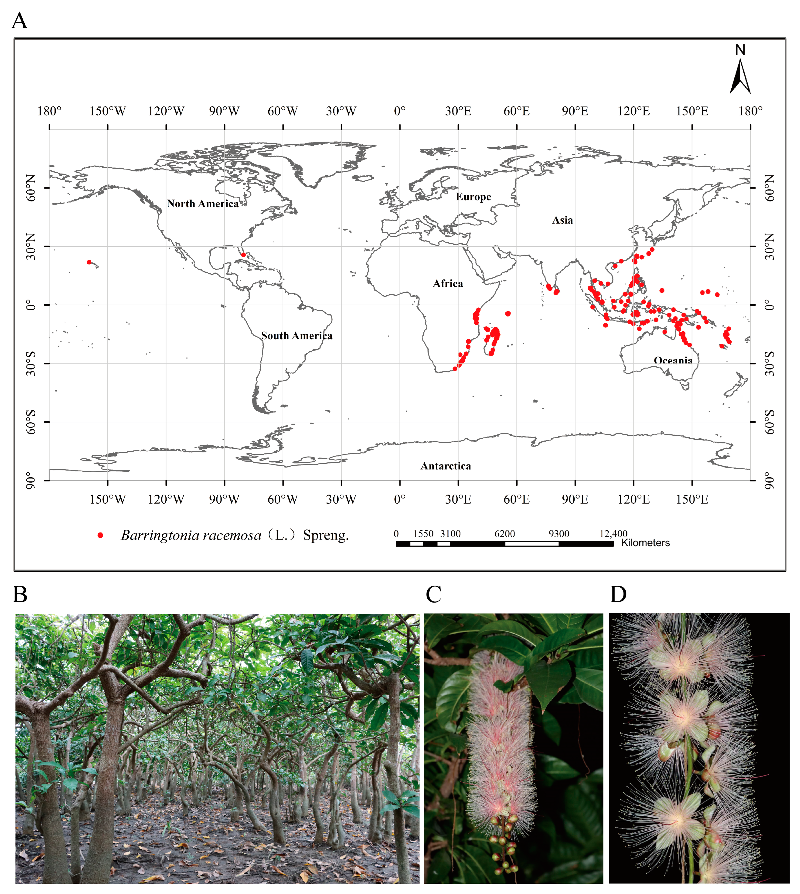
2.1. Data Collection of Barringtonia racemosa Distribution Points

The distribution points information of B. racemosa in this study comes from the Global Biodiversity Information Facility (GBIF) (https://www.gbif.org/, accessed on 29 October 2023) [41], Chinese Virtual Herbarium (CVH) (https://www.cvh.ac.cn/, accessed on 2 November 2023) [42], and the Royal Horticultural Society (RHS) (https://www.rhs.org.uk/, accessed on 2 November 2023) [43]. After retrieval, a total of 1014 distribution records of B. racemosa was obtained. Through https://coordinates-gps.gosur.com/cn/ (accessed on 6 November 2023), the longitude and latitude information of B. racemosa was determined, and the data without detailed geographic location, duplicate specimens, and location deviations were excluded. Finally, 144 geographical distribution points of B. racemosa were screened. We converted the obtained sample point data into .csv format and used ArcGIS 10.2 to draw a map of B. racemosa distribution in world map (Figure 1).

2.2. Environmental Variables

Barringtonia racemosa displays a unique growth pattern in the transition zone between terrestrial and marine habitats [44]. This study identified 33 environmental variables (Table 1) crucial for biological significance, such as climate, soil, topography, and marine factors, drawing from previous research and considering the ecological traits of B. racemosa. Climate data for 19 variables covering current climate (1970–2000) and projected future climate (2021–2040) were sourced from the World Climate Database (WorldClim) (https://www.worldclim.org/, accessed on 24 October 2023) [45]. Ten soil environmental variables were obtained from the World Soil Information (ISRIC) (https://data.isric.org/, accessed on 29 October 2023) [46] of the Food and Agriculture Organization of the United Nations, while three marine environmental variables were extracted from the Bio-ORACLE global marine life model environment database (https://www.bio-oracle.org/, accessed on 27 October 2023) [47]. The marine variables were calculated based on monthly average surface marine environment data from 2000 to 2014. The topographic elevation data (DEM) from the U.S. National Geophysical Data Center (NGDC) (https://www.ncei.noaa.gov/products/etopo-global-relief-model, accessed on 27 October 2023) [48] of the American Geophysical Center is imported into ArcGIS 10.2. It is essential for soil, topographic, and climate variables to match the resolution and scope of marine environmental data. All environmental variables’ raster data is converted into ASC format data files using the conversion tool in the Arc Tool Box [49].
In this study, the future bioclimatic data were derived from the BCC-CSM2-MR climate model of the sixth International Coupled Model Comparison Program (CMIP6), incorporating the shared socio-economic pathways (SSPs) and representative concentration pathways (RCPs) [50,51]. The potentially suitable growth zone of B. racemosa was simulated under three distinct concentration emission scenarios: SSP1-RCP2.6 (SSP126), SSP2-RCP4.5 (SSP245), and SSP5-RCP8.5 (SSP585). Among these, SSP126 represents a pathway towards sustainable development characterized by low levels of greenhouse gas emissions, while SSP245 embodies a more conventional approach with medium emissions levels. In contrast, SSP585 reflects a development trajectory reliant on fossil fuel utilization, resulting in high levels of greenhouse gas emissions [52,53]. Despite their differing emissions profiles, the future climate variable data for these scenarios underwent similar preprocessing procedures.

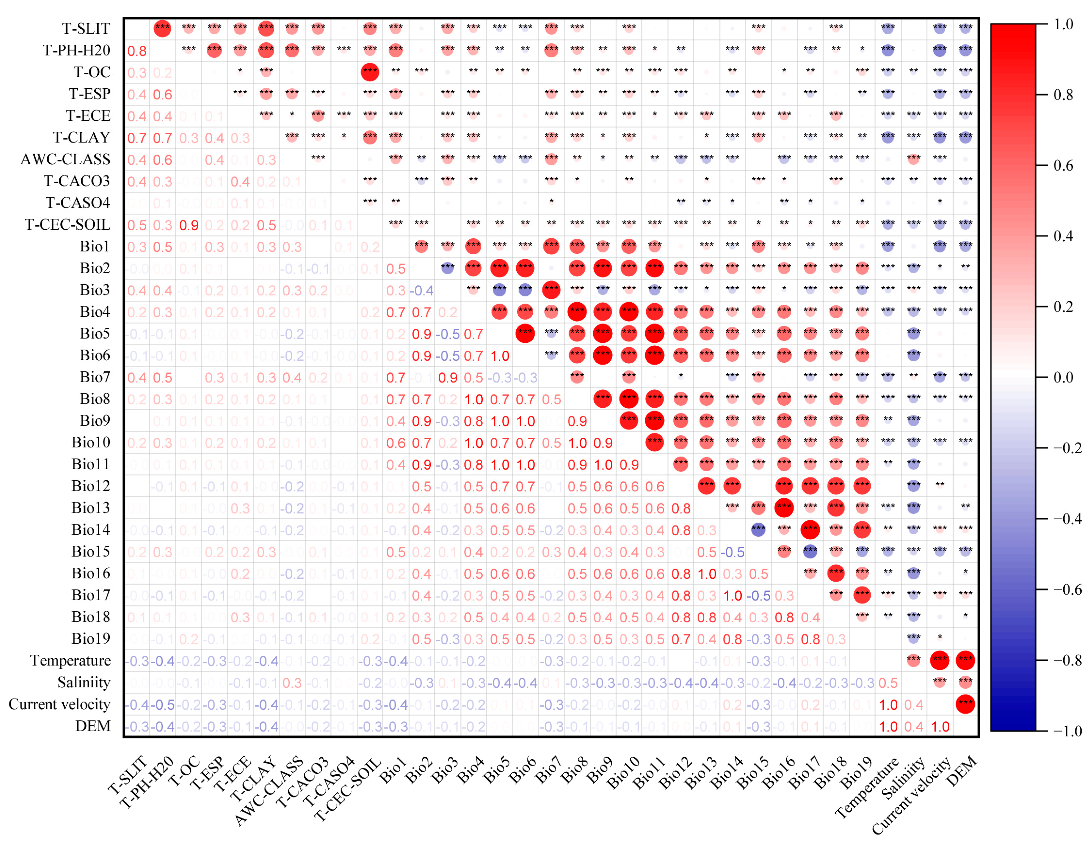
2.3. Environmental Variable Screening

The MaxEnt model predicts species distribution by inputting known geographical points and relevant environmental variables, while avoiding overfitting by considering collinearities among variables. This paper employed a knife-cutting analysis within the MaxEnt model and utilized the Pearson test (Figure 2) and R4.3.2 for visualization purposes, in order to eliminate environmental variables with a contribution value of less than 1% and low correlation within the initial model. The Pearson correlation coefficient is commonly utilized to assess the strength of linear correlation between variables and determine the presence and strength of a relationship between them [54]. In this study, all environmental variables exhibited significant or extremely significant correlations, with the majority displaying significant or extremely significant positive correlations. Notably, Temperature, Salinity, Current velocity, and DEM demonstrated significant or extremely negative correlations with other variables. Some environmental variables had a low but statistically significant correlation, while others did not show significant correlation. A high correlation coefficient suggests a strong relationship between the variables, but it may not be statistically significant due to potential random factors. Hence, it is imperative to conduct a comprehensive evaluation of the training model’s development by incorporating the specific percent contribution (PC). Variables with minimal contribution rates (PC < 1%) were subsequently eliminated [55], resulting in the selection of 11 environmental variables as the ultimate modeling parameters for the study (Table 2).

2.4. Species Distribution Modeling, Optimization, and Evaluation

Given the complexity of the MaxEnt model in machine learning, there is a need for further discussion on the authenticity and accuracy of simulating and predicting the distribution of potential complexity of an unknown species using a fixed algorithm. According to relevant research, model complexity, and feature combination (FC): LQPTH(L for linear liner, T for threshold, Q for quadratic type, H for fragmented hinge, and P for product type threshold) are significantly correlated with the regularization multiplier (RM) [56].
To mitigate the impact of overfitting on the model’s ability to migrate, the “Kuenm” package in R version 4.3.3 was utilized to assess the cross-combination of RM values ranging from 0 to 4, incremented by 0.5. The final model was selected based on the optimal parameter combination that yielded the smallest delta AICc value, representing the difference between the calibrated optimal model and the Akaike information criteria of the current model. This model demonstrated statistical significance, with an omission rate (OR) below 5% [57].
The global distribution data of B. racemosa and selected environmental variables were inputted into the MaxEnt software (Version 3.4.1). The program was executed using the Jackknife method to assess variable importance and determine the influence of environmental variables on global distribution. Response curves were generated to illustrate the correlation between environmental variables and the probability of B. racemosa distribution [58], and the output was formatted in logistic form. The basic parameter set option randomly selected 25% of the distribution points of B. racemosa as the test data and 75% as the training data, with 10 replicates of the model.
The model’s prediction accuracy was assessed using the Receiver Operating Characteristic (ROC) curve. The Area Under the Curve (AUC) values between 0.5 and 0.6 indicate failure, from 0.6 to 0.7 indicate poor results, from 0.7 to 0.8 indicate general results, from 0.8 to 0.9 indicate good results, and from 0.9 to 1 indicate excellent results [59]. In order to delineate the appropriate distribution areas with precision, the coastline was segmented into three categories (low, moderate, and high suitability) utilizing Jenks’s natural breaks methodology based on suitability values [60]. The data were then gathered and analyzed using ArcMap 10.5.

3. Results

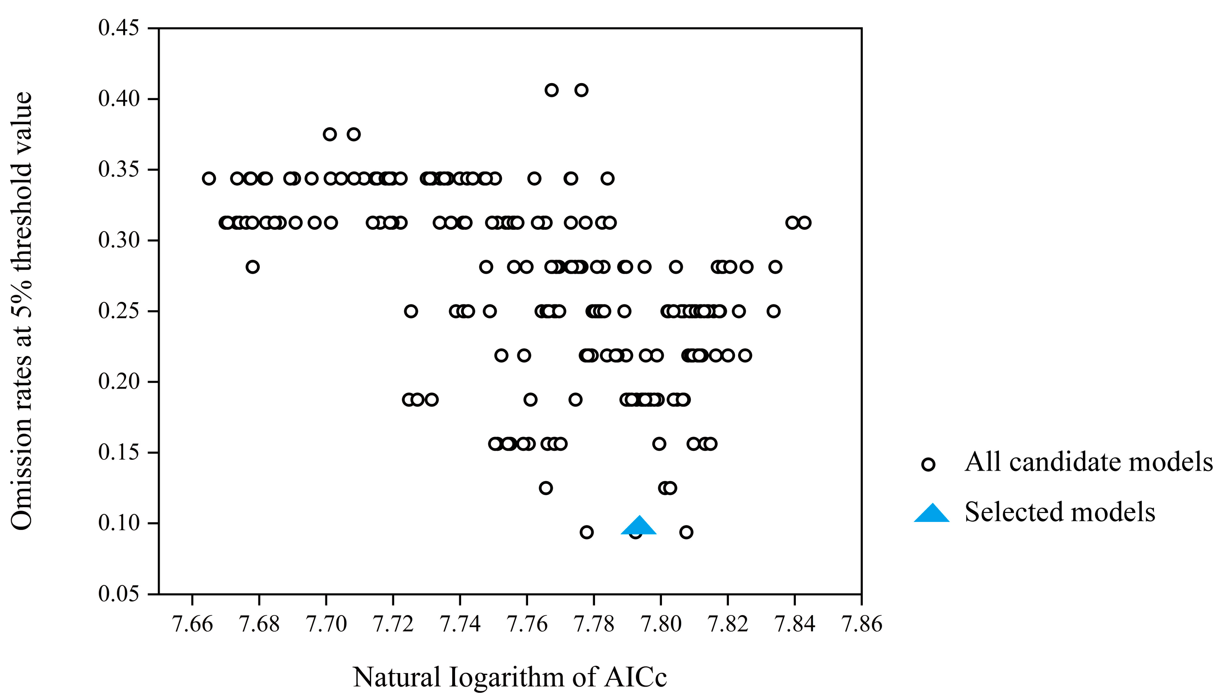
3.1. Model Optimization and Accuracy Evaluation Results

Using the optimized MaxEnt model, 144 Barringtonia racemosa distribution points and 11 environmental variable layers were selected to simulate the potential distribution area under different current and future scenarios (2040) according to the minimum information criterion (AICc). Based on the outcomes of model optimization, 144 unique combinations of model parameters were subjected to cross-validation by FC and RM. Among these combinations, one adheres to the criterion of omission rates (OR) being less than 5% and exhibiting a small delta AICc value. Specifically, FC selected Q+P+T, while the RM was set at 0.5. Currently, the omission rate stands at 3.4% with a delta AICc of 0, suggesting that the predictive accuracy of this particular parameter combination is superior (Figure 3) [61].
The MaxEnt simulations were conducted for both current and future (2040s) time frames under three distinct climate scenarios (SSP126, SSP245, and SSP585) using optimized parameters. The results of the simulations, as represented by the area under the receiver operating characteristic curve (AUC), are presented in Figure 4A–D, with all AUC values exceeding 0.95. These results demonstrate the exceptional predictive performance of the MaxEnt model, highlighting its high accuracy and reliability.

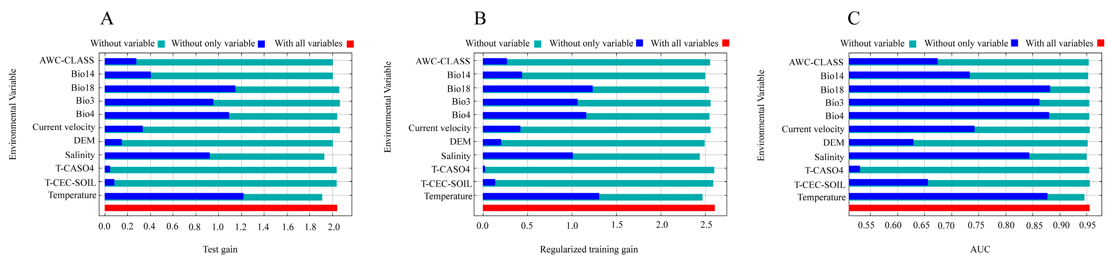
3.2. Dominant Environmental Variables of Potential Habitat Distribution of Barringtonia racemosa

Percent contribution (PC) and permutation importance (PI) are key metrics used to assess the significance of environmental variables. A higher index value indicates greater importance of the environmental variables being evaluated [50]. Table 3 illustrates that Temperature, Salinity, Bio18, Bio14, and DEM were among the top five contributors in both the current period and three future climate scenarios. Specifically, Temperature, Salinity, and Bio14 ranked among the top three contributors. The environmental variables with the highest percent contribution (PC) under the current environmental scenario were Temperature (39.1%), Salinity (17.9%), Bio18 (16.15%), Bio14 (7.2%), and DEM (5%), totaling 85.3%. The top five environmental variables in permutation importance (PI) were Temperature (59.9%), Salinity (10.1%), Bio4 (8.1%), Bio14 (6.2%), and Bio3 (3%), totaling 88.3%.
The results of the Jackknife test (Figure 5A–C) indicated that there was no significant difference in test gain, regularized training gain, and AUC when comparing models with no variables to those with all variables included. However, when only variables were utilized, the top five factors influencing test gain, regularization training gain, and AUC were identified as Bio18, Bio4, Temperature, Bio3, and Salinity, suggesting that these environmental factors play a crucial role in determining the distribution of B. racemosa. The comprehensive analysis of environment variables, including PC value, PI value, and Jackknife test results, indicates that Temperature, Salinity, Bio18, Bio14, Bio4, and Bio3 are the primary factors influencing the distribution of B. racemosa.

3.3. Response of Potential Distribution of Barringtonia racemosa to Main Environmental Variables

The species response curve illustrates the correlation between environmental factors and the likelihood of species occurrence, demonstrating species tolerance to environmental variables and habitat preference selection. To more accurately depict the influence of different environmental variables on the natural distribution of B. racemosa, the aforementioned variables (Temperature, Salinity, Bio18, Bio14, Bio4, and Bio3) with significant contribution rates were individually modeled as one-factor analyses. Simultaneously, the response curve depicting the relationship between the distribution probability of B. racemosa and key environmental variables is plotted based on the species’ probability of existence output by the model. Specifically, Figure 6 illustrates the response curve of six prominent environmental variables with occurrence probabilities exceeding 0.5. The threshold value of B. racemosa for each environmental variable can be determined.
The findings indicate that, based on the response curve generated by the optimized MaxEnt model, the optimal average ocean surface water temperature (Temperature) ranged from 15 °C to 35 °C, with the peak temperature being approximately 25 °C. Within the temperature range from 25 to 30 °C, the likelihood of B. racemosa distribution initiation decreased, while the probability stabilized at 0.5–0.6 within the temperature range from 30 to 35 °C (Figure 6A). The salinity levels exhibited variability between 5 and 25‰, with an optimal value of approximately 15‰. A notable decline in the natural distribution probability of B. racemosa was observed when salinity levels fell within the range from 18 to 25‰ (Figure 6B). The range of Bio18 spanned from 200 mm to 2000 mm, with the natural distribution probability of B. racemosa showing an increasing trend, peaking at approximately 1200 mm. Upon reaching levels from 1800 to 2000 mm, the distribution probability stabilized at around 0.7 (Figure 6C). Conversely, Bio14 ranged from 0 to 400 mm, with the optimal value falling within the range from 150 to 200 mm. Within the range from 200 to 400 mm, the distribution probability of B. racemosa remained stable at approximately 0.6 (Figure 6D). The range of Bio4 spanned from −200 to 2300, with an optimal value of approximately 250. Beyond this threshold, the distribution probability of B. racemosa experienced a significant decrease, and when Bio4 surpassed 750, the distribution probability approached zero (Figure 6E). Bio3 ranged from approximately 2 to 84, with an optimal value of around 50. When exceeding 60, the distribution probability of B. racemosa sharply decreased to 0.2 and stabilized (Figure 6F).

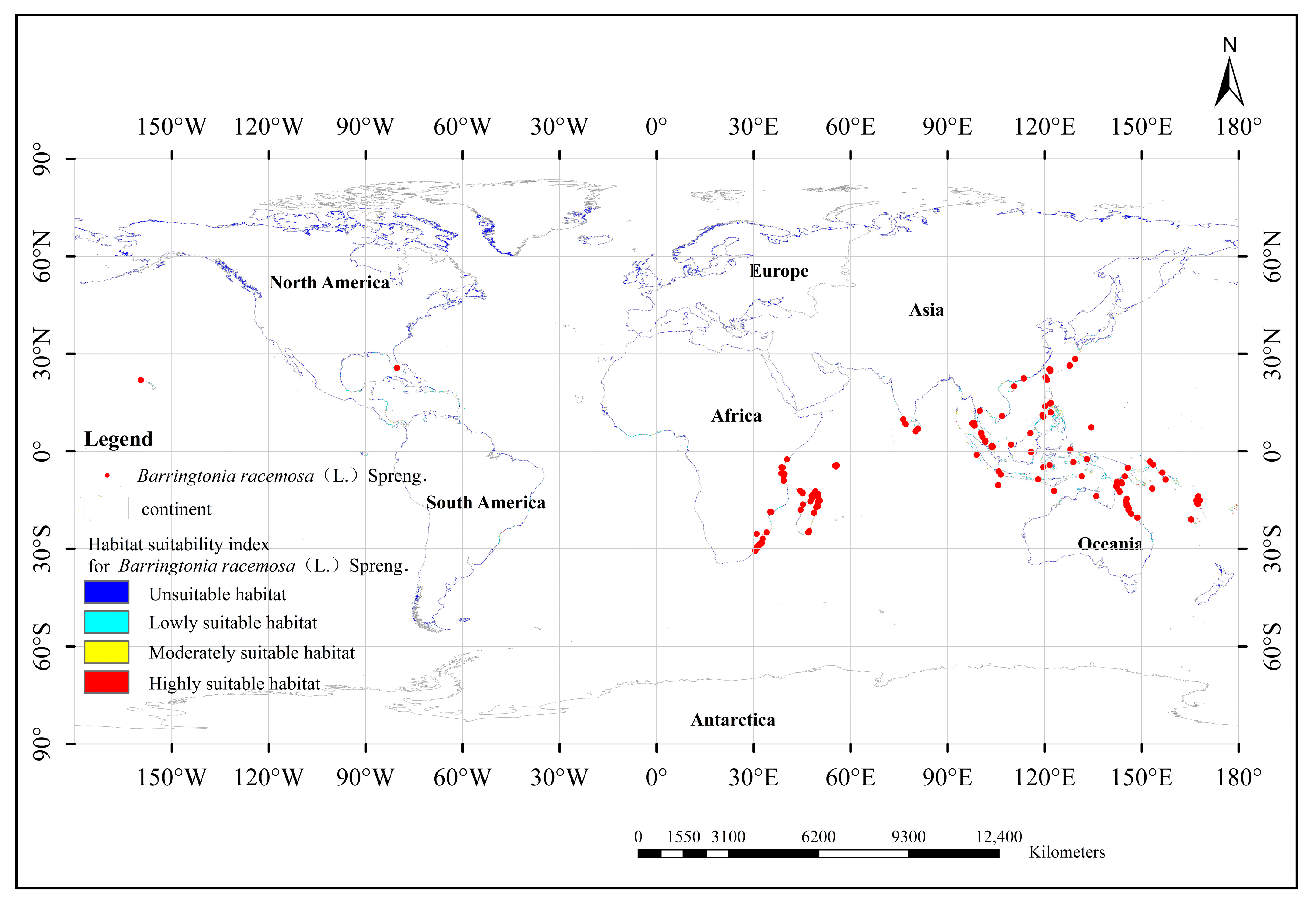
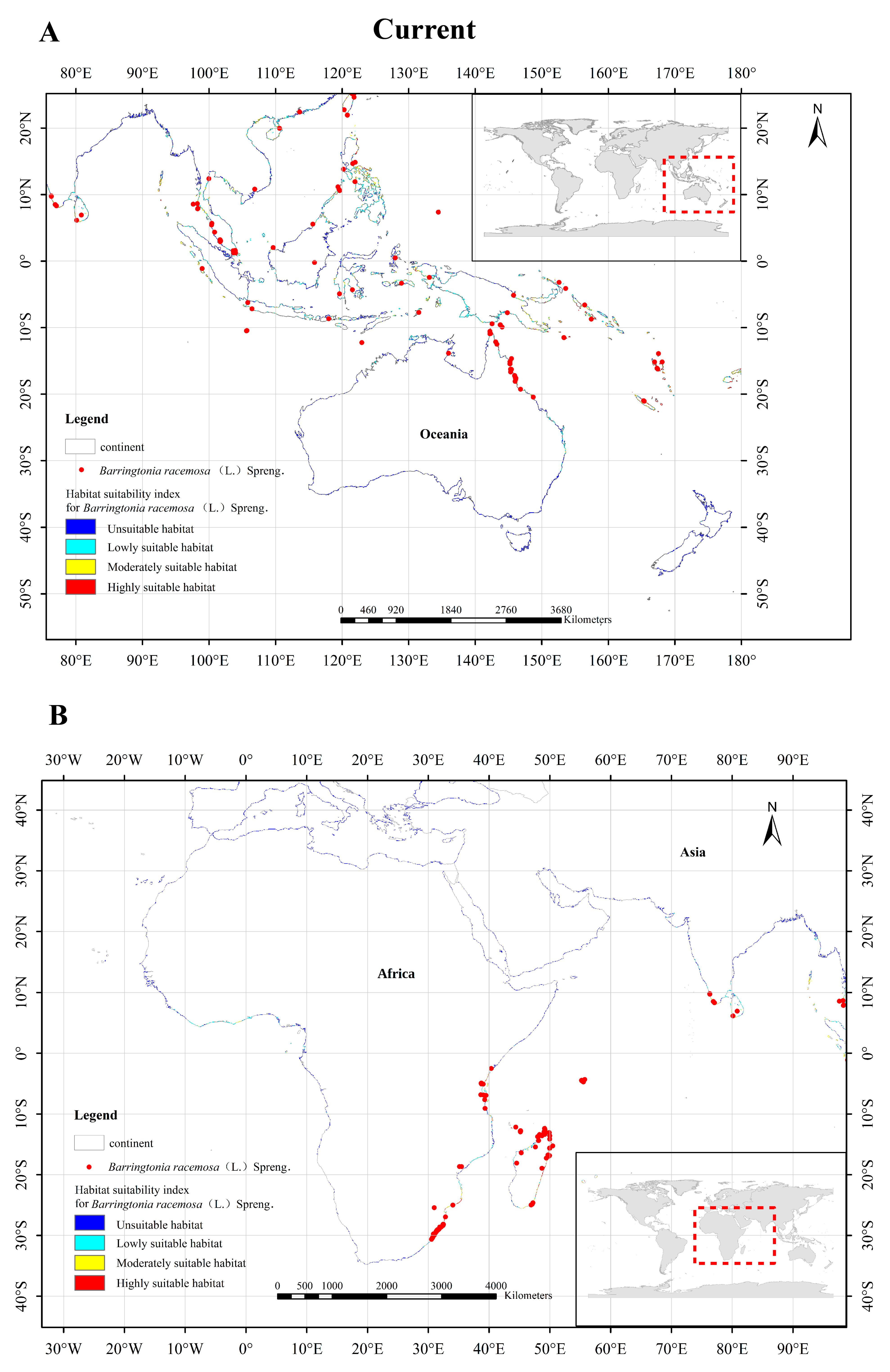
3.4. Distribution of Potential Suitable Growth Areas of Barringtonia racemosa in the Current Climate

The optimized MaxEnt model indicates that, based on current climate conditions, the distribution of B. racemosa habitats is primarily concentrated in tropical and subtropical coastal regions near the equator, encompassing a total area of 246.03 km2. This distribution includes high, middle, low, and unsuitable areas measuring 3.90 km2, 8.57 km2, 16.94 km2, and 216.63 km2, respectively, accounting for 1.58%, 3.48%, 6.88%, and 88.05% of the total suitable area (Table 4). Notably, the suitable habitats were predominantly found in Africa, Asia, and Oceania (Figure 7).
The regions in Asia that are particularly well suited for B. racemosa include the southern coastal areas of Zhanjiang, China, Taiwan, Vietnam, Myanmar, Malaysia, Singapore, the Nusa Tenggara Islands, the East Timor Islands, and New Guinea Island. Some moderately suitable areas include the southern coast of Guangdong and Guangxi in China, the eastern and western coasts of Taiwan, the southern coast of Andaman Islands, Mentawai Islands, Sumatra Island, Java Island, Nusa Tenggara Islands, East Timor Islands, New Guinea Island, Sulawesi, and the eastern, southern, and western coasts of the Philippines. Areas with low suitability include the southern coast of Guangdong in China, the eastern and southern coasts of Vietnam, the southwestern coast of Cambodia, the southern coast of Thailand, the southern coast of Myanmar, the eastern coast of Malaysia, the coast of Sumatra, the northern coast of Java, the Nusa Tenggara Islands, Kalimantan Island, Sulawesi Island, and the coasts of the Rougu Islands and New Guinea Island in Malaysia (Figure 8A).
The regions of high suitability for B. racemosa in Oceania encompass the eastern coast of New Ireland, the southern coast of Papua New Guinea, the coast of Tagula Island, the coast of the Solomon Islands, the coast of New Caledonia, the coast of Vanuatu Islands, the coast of Fiji Island, the northeastern coast of Australia, and the southwestern coast of New Caledonia. Moderately suitable areas include the coasts of Papua New Guinea, Solomon Islands, New Guinea, and eastern Australia. Areas of low suitability include the coastal coast of Papua New Guinea Islands, the coastal coast of Solomon Islands, the coastal coast of Eastern Australia, and the coastal coast of Fiji Island (Figure 8A).
In Africa, the middle and high suitable areas of B. racemosa include the eastern coastal coast of Tanzania, the coastal coast of Pemba Island, the eastern coastal coast of Kenya, the eastern coastal coast of South Africa, the eastern coast of Madagascar Island, the coastal coast of Mozambique, and the coastal coast of the Comoros Islands (Figure 8B). These regions are situated within a tropical rainforest climate characterized by consistently high temperatures and precipitation levels throughout the year. The minimal annual temperature fluctuations in these areas align with the optimal growth requirements of B. racemosa.

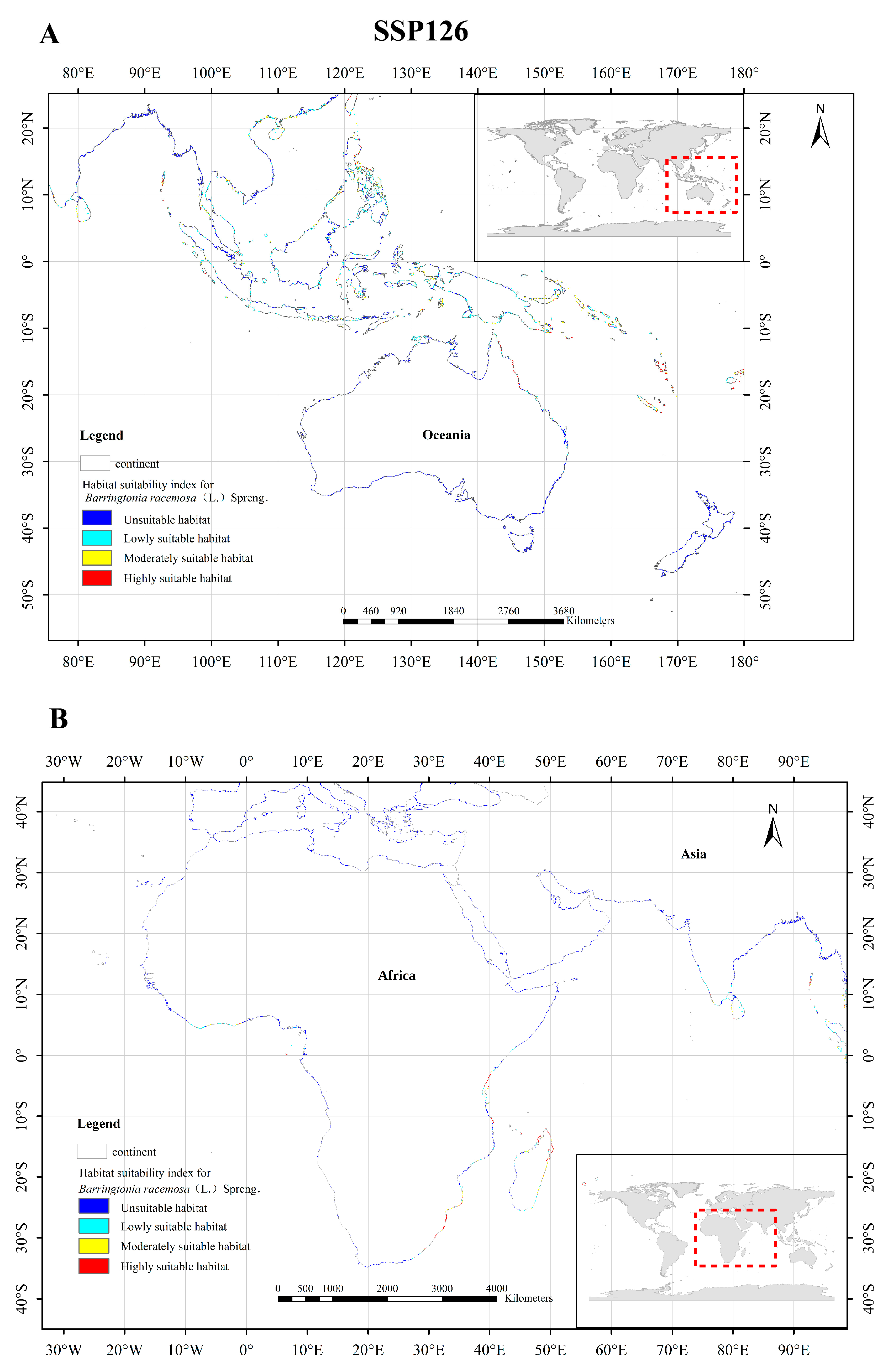
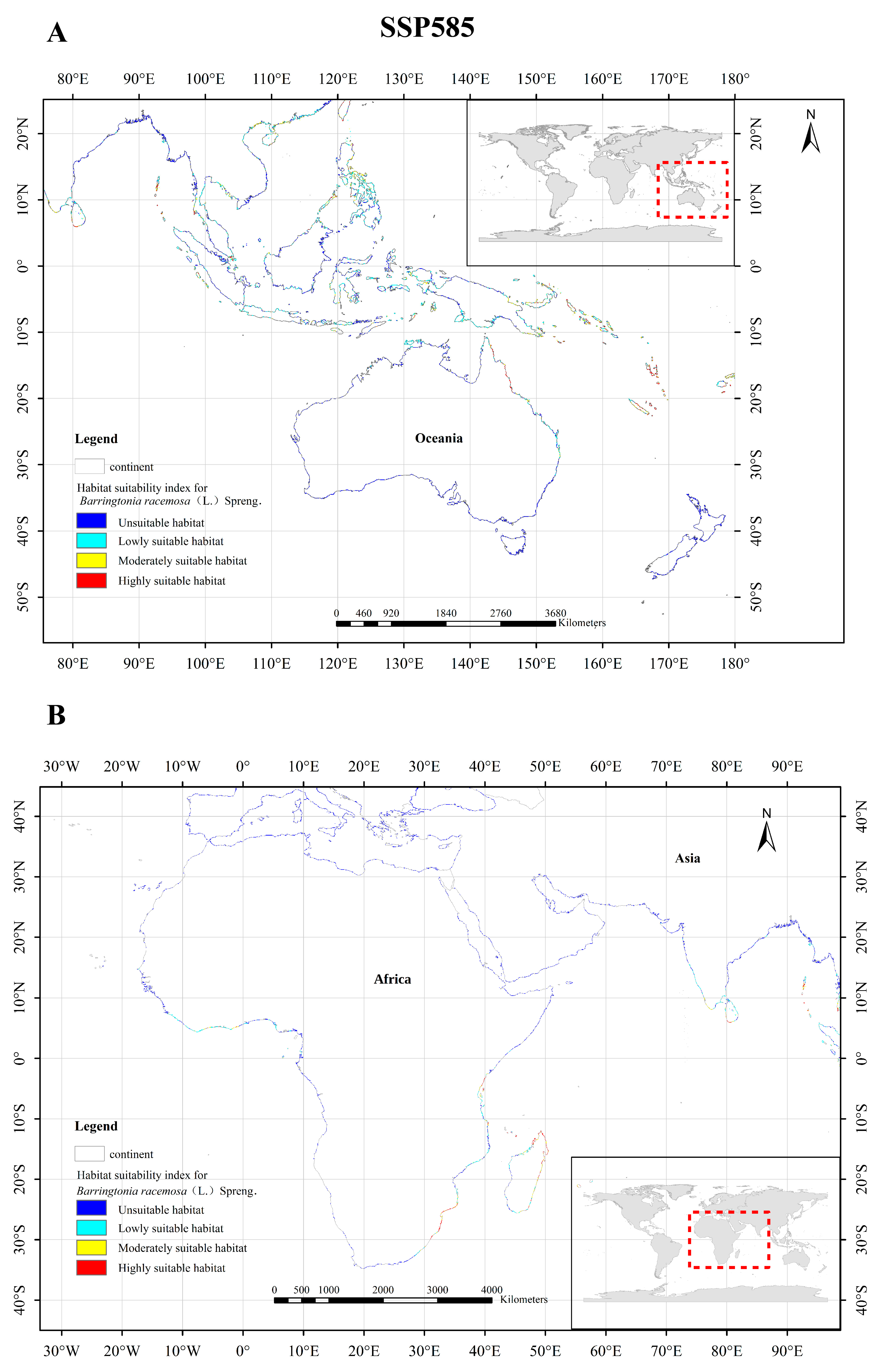
3.5. Changes of Potentially Suitable Zones of Barringtonia racemosa under Different Scenarios

Based on the findings of the optimized MaxEnt model, the potential distribution area of B. racemosa exhibited notable changes across three climate scenarios (SSP126, SSP245, and SSP585) as depicted in Figure 9, Figure 10 and Figure 11. These changes were primarily concentrated in Asia, Africa, and Oceania, with a slight increase observed in both low and high suitable areas.
Under the SSP126 climate scenario, changes in highly suitable areas for B. racemosa were observed in various regions of Asia, particularly in the coastal areas of Hainan and southern Taiwan in China, the coastal areas of eastern Philippines, the coastal areas of East Timor, and the coastal areas of southern Indonesia (Figure 9A). The alterations in highly suitable habitats for B. racemosa in Oceania were primarily focused on the southeastern coastal regions of Papua New Guinea, the coastal areas of the Solomon Islands, the coastal regions of Vanuatu, and the northeastern coast of Australia (Figure 9A). Similarly, in Africa, the changes in highly suitable habitats for B. racemosa were concentrated along the eastern coast of Tanzania, the eastern coast of Kenya, the southeastern coast of South Africa, and the coast of Madagascar (Figure 9B).
Under the SSP245 climate scenario, B. racemosa shifted to highly suitable areas in Asia, including the northern and southern coastal coasts of Taiwan and China, as well as the eastern coastal coasts of the Philippine Islands (Figure 10A). In Oceania, the plant’s suitable areas moved to the southeastern coastal coast of Papua New Guinea, the Solomian Islands, the Vanuatu Islands, the Fiji Islands, and the northeastern Islands of Australia (Figure 10A). The alterations in the distribution of highly suitable habitats for B. racemosa in Africa were primarily localized along the eastern coastal regions of Tanzania, Kenya, and South Africa, as well as the coast of Madagascar (Figure 10B).
In the context of the SSP585 climate scenario, B. racemosa exhibited alterations in areas deemed highly suitable in Asia, particularly along the coastal regions of southwest Thailand, the Sumatra Islands, the eastern Philippine Islands, and the southeastern East Timor Islands (Figure 11A). Similarly, in Oceania, the changes in highly suitable areas for B. racemosa were primarily observed along the southeastern coastal regions of Papua New Guinea, the Solomian Islands, the Vanuatu Islands, and the Fiji Island, among others (Figure 11A). Barringtonia racemosa’s changes in highly suitable areas in Africa were mainly concentrated in the eastern coastal coast of Mozambique, the eastern coastal coast of Kenya, the eastern coastal coast of South Africa, and the northeastern and eastern coasts of Madagascar (Figure 11B).
In comparison to the prevailing climate prediction outcomes, the potential total viable area and high viable area of B. racemosa are anticipated to expand under future climate scenarios. Specifically, in the SSP126 scenario, the total suitable area of B. racemosa was measured at 247.65 km², with the high suitable area encompassing 3.76 km², representing 1.52% of the total area. In contrast to the current climate scenario, the total suitable area of B. racemosa is projected to increase by 1.62 km², while the high suitable area is expected to decrease by 0.13 km². In the SSP245 scenario, the total suitable area for B. racemosa was measured at 247.65 km², with a high suitable area of 4.44 km², representing 1.79% of the total area. In comparison to the current climate scenario, there was an increase of 1.62 km² in the total suitable area and 0.54 km² in the high suitable area. In the context of the SSP585 scenario, the total suitable area of B. racemosa was measured at 247.65 km², with a high suitable area of 4.37 km², representing 1.79% of the total area. In comparison, under the contemporary climate scenario, both the total and highly suitable areas of B. racemosa experienced an increase of 1.62 km² and 0.47 km², respectively (Table 4).
In conclusion, the total suitable area of B. racemosa remains consistent under SSP126, SSP245, and SSP585. It is anticipated that the optimal habitat area will experience a slight increase in the future under these three emission scenarios compared to the present conditions. One possible explanation for the viability of B. racemosa may be attributed to its inherent biological characteristics, such as resistance to light and heat, enabling it to adapt to the effects of global warming. Alternatively, it is plausible that changes in external environmental conditions are aligning with the growth requirements of B. racemosa, thereby enhancing its overall viability.

4. Discussion

4.1. Dominant Environmental Factors Influencing the Suitability of Barringtonia racemosa

This study employed the Jackknife, AUC, PC, and PI tests in conjunction with the optimized MaxEnt model to determine the primary environmental factors influencing the distribution of B. racemosa. These factors were determined to include the ocean surface temperature (Temperature), average salinity of the ocean surface (Salinity), precipitation during the warmest quarter (Bio18), precipitation of the driest month (Bio14), seasonal variation coefficient of temperature (Bio4), and isothermality (Bio3) in the study area. Temperature plays a crucial role in plant growth and distribution, serving as a determining ecological factor. B. racemosa, a semi-mangrove plant, exhibits adaptability to both intertidal and terrestrial environments. Research indicates that the optimal temperature range for photosynthesis in mangrove leaves is 28~32 °C [62]. Various research studies have indicated that the zonal distribution of mangrove plants is influenced by air temperature and water temperature [63], with optimal temperatures being conducive to the growth of these plants. B. racemosa tolerates dry conditions but is intolerant of any frost. Specifically, our study concludes that the best water temperature range for B. racemosa was 25 °C, Additionally, a stable probability distribution of 0.5~0.6 was observed at temperatures in the range of 30~35 °C (Figure 6A), aligning with the natural habitat temperature distribution of B. racemosa.
Currently, an increasing number of studies indicate that global warming exhibits varying diurnal and seasonal warming rates [64,65]. For instance, the rate of global warming typically accelerates more rapidly during nighttime hours compared to daytime [65]. The temperature increase rate in summer was faster than that in spring and autumn, and the seasonal temperature difference showed a decreasing trend [66]. In temperate regions, vegetation typically displays discernible seasonal variations in photosynthetic activity [67]. The relationship between vegetation growth and temperature change exhibits seasonal variability [68,69]. In the present study, it was observed that when the seasonal variation coefficient of temperature (Bio4) exceeded approximately 750, there was a notable absence of natural distribution of B. racemosa (Figure 6E), suggesting that seasonal temperature fluctuations have a significant impact on the habitat of B. racemosa.
Similarly, the isothermality ratio serves as a metric for assessing temperature consistency within a given geographical area or time period. A greater ratio indicates reduced temperature variability, which may have positive implications for plant growth and development [70]. In this research, it was observed that the probability of occurrence of B. racemosa was highest at a Bio3 value of approximately 50. However, as the Bio3 value exceeded 60, the distribution probability of B. racemosa significantly decreased to 0.2 and stabilized (Figure 6F). While a high isothermal ratio can mitigate the harm inflicted on plants by extreme temperatures, it may also impede the growth cycle and adaptability of plants. Consequently, the suitable habitat of the B. racemosa population gradually contracted until it ultimately faced extinction.
Furthermore, research has indicated that precipitation during the rainy season has an impact on the distribution of mangroves [71]. It is generally accepted that higher levels of rainfall contribute to the expansion of mangrove habitats [72]. However, excessive rainfall during the wet season may result in elevated sea levels and pose challenges to the resilience of mangrove ecosystems during the warmest months [73]. Based on the findings of Liang Fang et al. [74], prolonged inundation is shown to diminish photosynthesis and respiration, consequently impacting the growth, development, and biomass accumulation of B. racemosa. In this study, when the precipitation of the warmest quarter (Bio18) was about 1200 mm, the occurrence probability of B. racemosa was as high as 0.8. However, Bio18 data showed a stable distribution of about 0.7 probability of B. racemosa at 1800~2000 mm (Figure 6C), which decreased slightly. This phenomenon may be attributed to an increase in rainfall and low temperatures. In such low-temperature conditions, B. racemosa may not receive adequate light and heat, ultimately impacting its biomass accumulation. When the precipitation of the driest month (Bio14) values ranged from 200 mm to 400 mm, the variation rate of B. racemosa was as high as 0.6 and tended to be stable (Figure 6D), potentially attributable to elevated temperatures in certain tropical or subtropical regions. Nations like South Africa experience hot and arid conditions influenced by tropical climates [75].
Excessive heat and ongoing sea water evaporation can elevate salinity levels, thereby impacting the dispersion of mangroves [76]. Mangrove plants possess a specialized salt tolerance mechanism to acclimate to saline environments; however, excessive salinity can impede plant development [77]. Optimal salinity levels are necessary to facilitate the growth and maturation of mangrove plants. Research has indicated that the species Kandelia candel (L.) Druce thrives within a seawater salinity range from 10‰ to 20‰ [78]. Barringtonia racemosa demonstrates optimal growth within a salinity range of 0~15‰, with some degree of tolerance observed up to 20~25‰; however, growth is significantly impeded at salinity levels exceeding 30‰ [79]. In this study, it was found that the natural distribution probability of B. racemosa was 0.7 at a salinity value of approximately 15‰ but decreased to nearly 0 within a salinity range of 18~25‰ (Figure 6B), consistent with the experimental results of Tan et al. [79] and Liang et al. [80]. In addition, when the rainy season arrives in the driest month, it rains in coastal areas of some countries, helping alleviate seawater evaporation and high salinity. This promotes the growth of B. racemosa and expands its distribution area. However, it may also explain why ocean surface salinity has a low impact on simulation results.

4.2. Possible Future Distribution of Barringtonia racemosa Based on Varying Climate Scenarios

Currently, mangroves are experiencing the impacts of climate change, resulting in a reduction in their distribution area and extent. To effectively safeguard the population resources of endangered mangroves and semi-mangroves, it is imperative to consider the spatial variations and ecological shifts in global mangrove distribution patterns on a macro scale. This study employed the MaxEnt model to predict the potential geographical distribution of B. racemosa under various future climatic emission concentration scenarios, namely SSP126, SSP245, and SSP585. The projected outcomes suggest that the total suitable habitat area for B. racemosa is expected to undergo a slight increase from 2021 to 2040 across three climatic emission scenarios in comparison to current conditions. Specifically, this increase is most notable under the middle- and high-emission scenarios (SSP245 and SSP585). It can be deduced that the habitat and ecological conditions of B. racemosa have been altered as a result of global warming, leading to the expansion of suitable growth areas for this species. This phenomenon may be attributed to the fact that B. racemosa is indigenous to tropical and subtropical regions and thrives in warmer climates. The practical implications of sea level rise as a consequence of global warming are expected to exacerbate habitat fragmentation and degradation, thereby increasing the vulnerability of seed breeding and seedling growth of B. racemosa. Factors such as the dispersal of B. racemosa fruit by the sea, the limited tolerance of seedlings to high salinity stress, and inhibited root growth may significantly compromise the reproductive success and survival of the species’ native population.
Furthermore, due to challenges in acquiring data pertaining to soil, topography, oceanic conditions, and other environmental variables in the future, this study exclusively utilized future climate variables to forecast the potential geographic range of B. racemosa. Nonetheless, the multifaceted and dynamic nature of factors influencing species distribution necessitates a comprehensive approach in order to more accurately assess and predict its suitable habitat, thereby acknowledging the limitations of the current prediction [81,82]. Barringtonia racemosa community within the mangrove ecosystem is a delicate plant species susceptible to various forms of disruption. Research conducted by Guo et al. [83] indicated that in the mangrove wetlands of the Leizhou Peninsula in China, disturbances primarily arise from plant invasions, river diversions, diseases, and insect pests. These disruptions have resulted in the degradation of ecosystem services, including water purification, oxygen generation, climate regulation, and carbon sequestration. In future research, we need to consider factors like biological invasion, river diversion, ports, and human interference to expand the model’s environmental variable screening. Several scholarly studies have indicated a decline in the population of mangrove B. racemosa in the Leizhou Peninsula [84]; during the field investigation of this study, it was observed that anthropogenic activities such as logging and the establishment of duck ponds and fish ponds have started to impede the natural growth of the wild population of B. racemosa in Suixi County, Zhanjiang City, Guangdong Province. Additionally, we should focus on conserving and utilizing areas suitable for B. racemosa growth to guide site selection for mangrove restoration during afforestation.

5. Conclusions

The MaxEnt model analysis has revealed that the potential distribution of B. racemosa is primarily concentrated in tropical and subtropical coastal regions near the equator, with a specific focus on regions in Africa, Asia, and Oceania. This prediction aligns closely with the known natural distribution of the species, indicating a continuous strip or band along coastal areas as the optimal habitat for B. racemosa.
Temperature-related variables (Temperature, Bio4, Bio3), precipitation-related variables (Bio18, Bio14), and salinity are the primary environmental factors influencing the distribution of B. racemosa. The analysis indicates that global warming, across various emission scenarios, could result in an expansion of the species’ range. This association underscores the importance of integrating environmental variables and habitat characteristics into conservation plans for B. racemosa in order to ensure the survival of this endangered species in mangrove ecosystems. By pinpointing critical environmental factors and appropriate habitats, stakeholders can formulate specific strategies to safeguard B. racemosa from the heightened risk of extinction posed by climate change. For instance, identifying optimal habitats for the strategic implementation of afforestation to enhance the range of B. racemosa distribution can be achieved. Spatial management of the native B. racemosa population can involve delineating ecological protection boundaries to regulate construction activities and anticipate associated risks. It is imperative to assess the potential negative impacts of development projects on B. racemosa growth and habitat, while also considering spatial variations and ecological shifts in the community’s distribution pattern. This research provides valuable insights that can inform conservation initiatives and help mitigate the impact of environmental changes on the endangered B. racemosa species.

Author Contributions

Conceptualization, F.L. and X.T.; methodology, Y.T. and Y.Y.; software, Y.T. and X.T.; formal analysis, F.L., X.Z. and X.X.; investigation, J.S., W.L., Z.D. and Y.W.; data curation, Y.T.; writing—original draft preparation, F.L. and Y.T.; writing—review and editing, X.T.; supervision, F.L. and X.Z.; project administration, F.L., X.T., Y.Y. and X.Z.; funding acquisition, F.L. All authors have read and agreed to the published version of the manuscript.

Funding

This research was funded by “The Natural Science Foundation of Guangxi Province, China, grant number 2022GXNSFBA035540”, “The National Natural Science Foundation of China, grant number 31660226”, “The Special Project for Basic Scientific Research of Guangxi Academy of Agricultural Sciences, grant number Guinongke 2021YT143”, The Special Project for Basic Scientific Research of Guangxi Academy of Agricultural Sciences, grant number Guinongke 2024YP134”, and the Project for Enhancing Young and Middle-aged Teachers’ Research Basic Ability in colleges of Guangxi, grant numbers 2021KY0592 and 2024KY0591.

Institutional Review Board Statement

Not applicable.

Data Availability Statement

The data supporting the findings of this study can be obtained upon request from the corresponding author, as they are not publicly accessible due to privacy concerns.

Acknowledgments

We express our gratitude to the reviewers for their insightful and valuable feedback, as well as to the editors for their assistance in enhancing the quality of this article.

Conflicts of Interest

The authors declare that they do not have any commercial or associative interest that represents a conflict of interest in connection with the work submitted.

References

  1. Linhares, Y.; Kaganski, A.; Agyare, C.; Kurnaz, I.A.; Neergheen, V.; Kolodziejczyk, B.; Kędra, M.; Wahajuddin, M.; El-Youssf, L.; Cruz, T.E.D.; et al. Biodiversity: The overlooked source of human health. Trends Mol. Med. 2023, 29, 173–187. [Google Scholar] [CrossRef] [PubMed]
  2. Tavilla, G.; Crisafulli, A.; Ranno, V.; Picone, R.M.; Redouan, F.Z.; del Galdo, G.G. First contribution to the ethnobotanical knowledge in the Peloritani Mounts (NE Sicily). Res. J. Ecol. Environ. Sci. 2022, 2, 1–34. [Google Scholar] [CrossRef]
  3. Bellard, C.; Bertelsmeier, C.; Leadley, P.; Thuiller, W.; Courchamp, F. Impacts of climate change on the future of biodiversity. Ecol. Lett. 2012, 15, 365–377. [Google Scholar] [CrossRef] [PubMed]
  4. Urban, M.C. Accelerating extinction risk from climate change. Science 2015, 348, 571–573. [Google Scholar] [CrossRef] [PubMed]
  5. Booth, T.H. Biodiversity and Climate Change Adaptation in Australia: Strategy and Research Developments. Adv. Clim. Chang. Res. 2012, 3, 12–21. [Google Scholar] [CrossRef]
  6. Sorte, C.J.B.; Ibáñez, I.; Blumenthal, D.M.; Molinari, N.A.; Miller, L.P.; Grosholz, E.D.; Diez, J.M.; D’Antonio, C.M.; Olden, J.D.; Jones, S.J.; et al. Poised to prosper? A cross-system comparison of climate change effects on native and non-native species performance. Ecol. Lett. 2013, 16, 261–270. [Google Scholar] [CrossRef] [PubMed]
  7. Aroloye, O.N. Mangrove Habitat Loss and the Need for the Establishment of Conservation and Protected Areas in the Niger Delta, Nigeria. In Habitats of the World; Carmelo Maria, M., Ana Cano, O., Ricardo Quinto, C., Eds.; IntechOpen: Rijeka, Croatia, 2019; p. Ch. 4. [Google Scholar]
  8. Cano, E.; Cano-Ortiz, A.; Veloz, A.; Alatorre, J.; Otero, R. Comparative analysis between the mangrove swamps of the Caribbean and those of the State of Guerrero (Mexico). Plant Biosyst.-Int. J. Deal. All Asp. Plant Biol. 2012, 146, 112–130. [Google Scholar] [CrossRef]
  9. Atwood, T.B.; Connolly, R.M.; Almahasheer, H.; Carnell, P.E.; Duarte, C.M.; Lewis, C.J.E.; Irigoien, X.; Kelleway, J.J.; Lavery, P.S.; Macreadie, P.I.; et al. Global patterns in mangrove soil carbon stocks and losses. Nat. Clim. Chang. 2017, 7, 523–528. [Google Scholar] [CrossRef]
  10. Hoekstra, J.M.; Boucher, T.M.; Ricketts, T.H.; Roberts, C. Confronting a biome crisis: Global disparities of habitat loss and protection. Ecol. Lett. 2004, 8, 23–29. [Google Scholar] [CrossRef]
  11. Graham, E.M.; Reside, A.E.; Atkinson, I.; Baird, D.; Hodgson, L.; James, C.S.; VanDerWal, J.J. Climate change and biodiversity in Australia: A systematic modelling approach to nationwide species distributions. Australas. J. Environ. Manag. 2019, 26, 112–123. [Google Scholar] [CrossRef]
  12. Yan, G.; Zhang, G. Predicting the Potential Distribution of Endangered Parrotia subaequalis in China. Forests 2022, 13, 1595. [Google Scholar] [CrossRef]
  13. Eiserhardt, W.L.; Svenning, J.-C.; Kissling, W.D.; Balslev, H. Geographical ecology of the palms (Arecaceae): Determinants of diversity and distributions across spatial scales. Ann. Bot. 2011, 108, 1391–1416. [Google Scholar] [CrossRef] [PubMed]
  14. Wasowicz, P.; Przedpelska-Wasowicz, E.M.; Kristinsson, H. Alien vascular plants in Iceland: Diversity, spatial patterns, temporal trends, and the impact of climate change. Flora 2013, 208, 648–673. [Google Scholar] [CrossRef]
  15. Lippmann, R.; Babben, S.; Menger, A.; Delker, C.; Quint, M. Development of Wild and Cultivated Plants under Global Warming Conditions. Curr. Biol. 2019, 29, R1326–R1338. [Google Scholar] [CrossRef] [PubMed]
  16. Selwood, K.E.; McGeoch, M.A.; Mac Nally, R. The effects of climate change and land-use change on demographic rates and population viability. Biol. Rev. 2015, 90, 837–853. [Google Scholar] [CrossRef] [PubMed]
  17. Román-Palacios, C.; Wiens, J.J. Recent responses to climate change reveal the drivers of species extinction and survival. Proc. Natl. Acad. Sci. USA 2020, 117, 4211–4217. [Google Scholar] [CrossRef] [PubMed]
  18. Thakur, S.; Rai, I.D.; Singh, B.; Dutt, H.C.; Musarella, C.M. Predicting the suitable habitats of Elwendia persica in the Indian Himalayan Region (IHR). Plant Biosyst.-Int. J. Deal. All Asp. Plant Biol. 2023, 157, 769–778. [Google Scholar] [CrossRef]
  19. Nan, Q.; Li, C.; Li, X.; Zheng, D.; Li, Z.; Zhao, L. Modeling the Potential Distribution Patterns of the Invasive Plant Species Phytolacca americana in China in Response to Climate Change. Plants 2024, 13, 1082. [Google Scholar] [CrossRef]
  20. Kamyo, T.; Asanok, L. Modeling habitat suitability of Dipterocarpus alatus (Dipterocarpaceae) using MaxEnt along the Chao Phraya River in Central Thailand. For. Sci. Technol. 2020, 16, 1–7. [Google Scholar] [CrossRef]
  21. Abdelaal, M.; Fois, M.; Fenu, G.; Bacchetta, G. Using MaxEnt modeling to predict the potential distribution of the endemic plant Rosa arabica Crép. in Egypt. Ecol. Inform. 2019, 50, 68–75. [Google Scholar] [CrossRef]
  22. He, K.; Fan, C.; Zhong, M.; Cao, F.; Wang, G.; Cao, L. Evaluation of Habitat Suitability for Asian Elephants in Sipsongpanna under Climate Change by Coupling Multi-Source Remote Sensing Products with MaxEnt Model. Remote. Sens. 2023, 15, 1047. [Google Scholar] [CrossRef]
  23. Wang, Y.; Chao, B.; Dong, P.; Zhang, D.; Yu, W.; Hu, W.; Ma, Z.; Chen, G.; Liu, Z.; Chen, B. Simulating spatial change of mangrove habitat under the impact of coastal land use: Coupling MaxEnt and Dyna-CLUE models. Sci. Total Environ. 2021, 788, 147914. [Google Scholar] [CrossRef] [PubMed]
  24. Mousazade, M.; Ghanbarian, G.; Pourghasemi, H.R.; Safaeian, R.; Cerdà, A. Maxent Data Mining Technique and Its Comparison with a Bivariate Statistical Model for Predicting the Potential Distribution of Astragalus Fasciculifolius Boiss. in Fars, Iran. Sustainability 2019, 11, 3452. [Google Scholar] [CrossRef]
  25. Li, L.; Liu, W.; Ai, J.; Cai, S.; Dong, J. Predicting Mangrove Distributions in the Beibu Gulf, Guangxi, China, Using the MaxEnt Model: Determining Tree Species Selection. Forests 2023, 14, 149. [Google Scholar] [CrossRef]
  26. Çoban, H.O.; Örücü, Ö.K.; Arslan, E.S. MaxEnt Modeling for Predicting the Current and Future Potential Geographical Distribution of Quercus libani Olivier. Sustainability 2020, 12, 2671. [Google Scholar] [CrossRef]
  27. Li, M.; Li, Q.; Song, J.; Wang, Z.; Wang, Y.; Hu, M. Prediction of potential distribution areas of Chinese horseshoe crab and mangrove horseshoe crab in the Beibu Gulf of Guangxi based on MAXENT model and their population conservation strategies. Acta Ecol. Sin. 2019, 39, 3100–3109. [Google Scholar] [CrossRef]
  28. Wang, G.; Xie, C.; Wei, L.; Gao, Z.; Yang, H.; Jim, C. Predicting Suitable Habitats for China’s Endangered Plant Handeliodendron bodinieri (H. Lév.) Rehder. Diversity 2023, 15, 1033. [Google Scholar] [CrossRef]
  29. Jiang, X.; Liu, W.-J.; Zhu, Y.-Z.; Cao, Y.-T.; Yang, X.-M.; Geng, Y.; Zhang, F.-J.; Sun, R.-Q.; Jia, R.-W.; Yan, C.-L.; et al. Impacts of Climate Changes on Geographic Distribution of Primula filchnerae, an Endangered Herb in China. Plants 2023, 12, 3561. [Google Scholar] [CrossRef] [PubMed]
  30. Rong, S.; Luo, P.; Yi, H.; Yang, X.; Zhang, L.; Zeng, D.; Wang, L. Predicting Habitat Suitability and Adaptation Strategies of an Endangered Endemic Species, Camellia luteoflora Li ex Chang (Ericales: Theaceae) under Future Climate Change. Forests 2023, 14, 2177. [Google Scholar] [CrossRef]
  31. Hu, W.; Wang, Y.; Zhang, D.; Yu, W.; Chen, G.; Xie, T.; Liu, Z.; Ma, Z.; Du, J.; Chao, B.; et al. Mapping the potential of mangrove forest restoration based on species distribution models: A case study in China. Sci. Total Environ. 2020, 748, 142321. [Google Scholar] [CrossRef]
  32. Cui, L.; Berger, U.; Cao, M.; Zhang, Y.; He, J.; Pan, L.; Jiang, J. Conservation and Restoration of Mangroves in Response to Invasion of Spartina alterniflora Based on the MaxEnt Model: A Case Study in China. Forests 2023, 14, 1220. [Google Scholar] [CrossRef]
  33. Ying, B.; Tian, K.; Guo, H.; Yang, X.; Li, W.; Li, Q.; Luo, Y.C.; Zhang, X.M. Predicting potential suitable habitats of Kandelia obovata in China under future climatic scenarios based on MaxEnt model. Acta Ecol. Sin. 2024, 44, 224–234. [Google Scholar] [CrossRef]
  34. Wang, Y.; Dong, P.; Hu, W.; Chen, G.; Zhang, D.; Chen, B.; Lei, G. Modeling the Climate Suitability of Northernmost Mangroves in China under Climate Change Scenarios. Forests 2022, 13, 64. [Google Scholar] [CrossRef]
  35. Jayathilake, D.R.; Costello, M.J. A modelled global distribution of the seagrass biome. Biol. Conserv. 2018, 226, 120–126. [Google Scholar] [CrossRef]
  36. Zellmer, A.J.; Claisse, J.T.; Williams, C.M.; Schwab, S.; Pondella, D.J. Predicting Optimal Sites for Ecosystem Restoration Using Stacked-Species Distribution Modeling. Front. Mar. Sci. 2019, 6, 3. [Google Scholar] [CrossRef]
  37. Aluri, J.S.R.; Palathoti, S.R.; Banisetti, D.K.; Samareddy, S.K. Pollination Ecology Characteristics of Barringtonia racemosa (L.) Spreng. (Lecythidaceae). Transylv. Rev. Syst. Ecol. Res. 2019, 21, 27–34. [Google Scholar] [CrossRef]
  38. Chantaranothai, P. Barringtonia (Lecythidaceae) in Thailand. Kew Bull. 1995, 50, 677. [Google Scholar] [CrossRef]
  39. Umaru, I.J.; Ahmed, F.B.; Umaru, H.A.; Umaru, K.I. Barringtonia racemosa: Phytochemical, pharmacological, biotechnological, botanical, traditional use and agronomical aspects. World J. Pharm. Pharm. Sci. 2018, 7, 78–121. [Google Scholar] [CrossRef]
  40. Lim, T.K. Barringtonia racemosa. In Edible Medicinal And Non Medicinal Plants: Volume 3, Fruits; Lim, T.K., Ed.; Springer: Dordrecht, The Netherlands, 2012; pp. 114–121. [Google Scholar]
  41. Global Biodiversity Information Facility. Global Biodiversity Information Facility (GBIF) Occurrence Download. 2023. Available online: https://www.gbif.org/occurrence/download/0173717-210914110416597 (accessed on 29 October 2023).
  42. Chinese Virtual Herbarium. Chinese Virtual Herbarium(CVH) Occurrence Download. 2023. Available online: https://www.cvh.ac.cn/ (accessed on 2 November 2023).
  43. Royal Horticultural Society. The Royal Horticultural Society (RHS) Occurrence Download. 2023. Available online: https://www.rhs.org.uk/ (accessed on 2 November 2023).
  44. Yang, F.; Ai, X.; Wang, C.; Cheng, L.; Feng, Q.; Sheng, N. Investigation on the Population Status of Rare and Endangered Tree Species Barringtonia racemosa in Liuniutan Wetland, Zhanjiang. Trop. For. 2023, 51, 66–69. [Google Scholar] [CrossRef]
  45. WorldClim, Maps, Graphs, Tables, and DATA of the Globla Climate. Available online: http://www.worldclim.org/ (accessed on 16 July 2020).
  46. World Soil Information. World Soil Information (ISRIC) Occurrence Download. 2023. Available online: https://data.isric.org/ (accessed on 29 October 2023).
  47. Bio-ORACLE. Bio-ORACLE Global Marine Life Model Environment Database Occurrence Download. 2023. Available online: https://www.bio-oracle.org/ (accessed on 27 October 2023).
  48. National Centers for Environmental Information. National Geophysical Data Center (NGDC) Occurrence Download. 2023. Available online: https://www.ncei.noaa.gov/products/etopo-global-relief-model (accessed on 17 November 2023).
  49. Hou, J.; Xiang, J.; Li, D.; Liu, X. Prediction of Potential Suitable Distribution Areas of Quasipaa spinosa in China Based on MaxEnt Optimization Model. Biology 2023, 12, 366. [Google Scholar] [CrossRef]
  50. Eyring, V.; Bony, S.; Meehl, G.A.; Senior, C.A.; Stevens, B.; Stouffer, R.J.; Taylor, K.E. Overview of the Coupled Model Intercomparison Project Phase 6 (CMIP6) experimental design and organization. Geosci. Model Dev. 2016, 9, 1937–1958. [Google Scholar] [CrossRef]
  51. O’neill, B.C.; Carter, T.R.; Ebi, K.; Harrison, P.A.; Kemp-Benedict, E.; Kok, K.; Kriegler, E.; Preston, B.L.; Riahi, K.; Sillmann, J.; et al. Achievements and needs for the climate change scenario framework. Nat. Clim. Chang. 2020, 10, 1074–1084. [Google Scholar] [CrossRef] [PubMed]
  52. Peng, S.; Wang, C.; Li, Z.; Mihara, K.; Kuramochi, K.; Toma, Y.; Hatano, R. Climate change multi-model projections in CMIP6 scenarios in Central Hokkaido, Japan. Sci. Rep. 2023, 13, 230. [Google Scholar] [CrossRef] [PubMed]
  53. Ebi, K.L.; Hallegatte, S.; Kram, T.; Arnell, N.W.; Carter, T.R.; Edmonds, J.; Kriegler, E.; Mathur, R.; O’Neill, B.C.; Riahi, K.; et al. A new scenario framework for climate change research: Background, process, and future directions. Clim. Chang. 2014, 122, 363–372. [Google Scholar] [CrossRef]
  54. Guo, L.; Guo, Z.; Jia, H.; Fan, R. Residents electric larceny detection based on Pearson correlation coefficient and SVM. J. Hebei Univ. 2023, 43, 357–363. [Google Scholar] [CrossRef]
  55. Wang, R.; Yang, H.; Luo, W.; Wang, M.; Lu, X.; Huang, T.; Zhao, J.; Li, Q. Predicting the potential distribution of the Asian citrus psyllid, Diaphorina citri(Kuwayama), in China using the MaxEnt model. PeerJ 2019, 7, e7323. [Google Scholar] [CrossRef] [PubMed]
  56. Zhu, G.; Qiao, H. Effect of the Maxent model’s complexity on the prediction of species potential distributions. Biodivers. Sci. 2016, 24, 1189–1196. [Google Scholar] [CrossRef]
  57. Cobos, M.E.; Townsend Peterson, A.; Barve, N.; Osorio-Olvera, L. kuenm: An R package for detailed development of ecological niche models using Maxent. PeerJ 2019, 7, e6281. [Google Scholar] [CrossRef]
  58. Wang, R.; Li, Q.; Wang, M. Climatic suitability regionalization of Actinidia chinensis in China. Acta Agric. Zhejiangensis 2018, 30, 1504–1512. [Google Scholar] [CrossRef]
  59. Merckx, B.; Steyaert, M.; Vanreusel, A.; Vincx, M.; Vanaverbeke, J. Null models reveal preferential sampling, spatial autocorrelation and overfitting in habitat suitability modelling. Ecol. Model. 2011, 222, 588–597. [Google Scholar] [CrossRef]
  60. North, M.A. A Method for Implementing a Statistically Significant Number of Data Classes in the Jenks Algorithm. In Proceedings of the 2009 Sixth International Conference on Fuzzy Systems and Knowledge Discovery, Tianjin, China, 14–16 August 2009; Volume 1, pp. 35–38. [Google Scholar]
  61. Radosavljevic, A.; Anderson, R.P. Making better Maxent models of species distributions: Complexity, overfitting and evaluation. J. Biogeogr. 2013, 41, 629–643. [Google Scholar] [CrossRef]
  62. Zhang, Q.; Sui, S.; Zhang, Y.; Yu, H.; Sun, Z.; Wen, X. Marine environmental indexes related to mangrove growth. Acta Ecol. Sin. 2001, 21, 1427–1437. [Google Scholar] [CrossRef]
  63. Wang, Y. Impacts, challenges and opportunities of global climate change on mangrove ecosystems. J. Trop. Oceanogr. 2021, 40, 1–14. [Google Scholar] [CrossRef]
  64. Easterling, D.R.; Horton, B.; Jones, P.D.; Peterson, T.C.; Karl, T.R.; Parker, D.E.; Salinger, M.J.; Razuvayev, V.; Plummer, N.; Jamason, P.; et al. Maximum and Minimum Temperature Trends for the Globe. Science 1997, 277, 364–367. [Google Scholar] [CrossRef]
  65. Davy, R.; Esau, I.; Chernokulsky, A.; Outten, S.; Zilitinkevich, S. Diurnal asymmetry to the observed global warming. Int. J. Climatol. 2017, 37, 79–93. [Google Scholar] [CrossRef]
  66. Xu, L.; Myneni, R.B.; Iii, F.S.C.; Callaghan, T.V.; Pinzon, J.E.; Tucker, C.J.; Zhu, Z.; Bi, J.; Ciais, P.; Tømmervik, H.; et al. Temperature and vegetation seasonality diminishment over northern lands. Nat. Clim. Chang. 2013, 3, 581–586. [Google Scholar] [CrossRef]
  67. Xia, J.; Chen, J.; Piao, S.; Ciais, P.; Luo, Y.; Wan, S. Terrestrial carbon cycle affected by non-uniform climate warming. Nat. Geosci. 2014, 7, 173–180. [Google Scholar] [CrossRef]
  68. Tan, J.; Piao, S.; Chen, A.; Zeng, Z.; Ciais, P.; Janssens, I.A.; Mao, J.; Myneni, R.B.; Peng, S.; Peñuelas, J.; et al. Seasonally different response of photosynthetic activity to daytime and night-time warming in the Northern Hemisphere. Glob. Chang. Biol. 2014, 21, 377–387. [Google Scholar] [CrossRef]
  69. Wu, X.; Liu, H.; Li, X.; Liang, E.; Beck, P.S.A.; Huang, Y. Seasonal divergence in the interannual responses of Northern Hemisphere vegetation activity to variations in diurnal climate. Sci. Rep. 2016, 6, 19000. [Google Scholar] [CrossRef]
  70. Cleland, E.E.; Allen, J.M.; Crimmins, T.M.; Dunne, J.A.; Pau, S.; Travers, S.E.; Zavaleta, E.S.; Wolkovich, E.M. Phenological tracking enables positive species responses to climate change. Ecology 2012, 93, 1765–1771. [Google Scholar] [CrossRef]
  71. Wei, X.; Shi, F.; Fan, J.; Yang, Q. Climate Change Impacts on Marine Lives and Ecosystems. Adv. Mar. Sci. 2011, 29, 241–252. [Google Scholar] [CrossRef]
  72. Yan, X.; Cai, R.; Guo, H.; Xu, W.; Tan, H. Vulnerability of Hainan Dongzhaigang mangrove ecosystem to the climate change. J. Appl. Oceanogr. 2019, 38, 338–349. [Google Scholar] [CrossRef]
  73. Ellison, J.C.; Stoddart, D.R. Mangrove ecosystem collapse during predicted sea-level rise: Holocene analogues and implications. J. Coast. Res. 1991, 7, 151–165. [Google Scholar]
  74. Fang, L.; Pan, Y.J.; Deng, X.; Wu, Y.; Liang, Z.; Zhao, S.; Tan, X. Responses of Barringtonia racemosa to Tidal Flooding. Fujian J. Agric. Sci. 2020, 35, 1346–1356. [Google Scholar] [CrossRef]
  75. Jagtap, T.G.; Nagle, V.L. Response and Adaptability of Mangrove Habitats from the Indian Subcontinent to Changing Climate. AMBIO 2007, 36, 328–334. [Google Scholar] [CrossRef] [PubMed]
  76. Huang, X.; Chen, Y.; Mo, W.; Fan, H.; Liu, W.; Sun, M.; Xie, M.; Xu, S.M. Climate change and its influence in Beibu Gulf mangrove biome of Guangxi in past 60 years. Acta Ecol. Sin. 2021, 41, 5026–5033. [Google Scholar] [CrossRef]
  77. Liao, B. The Adaptability of Seedlings of Three Mangrove Species to Tide-Flooding and Water Salinity; Chinese Academy of Forestry: Beijing, China, 2010. [Google Scholar]
  78. Chen, C.; Wang, W.; Lin, P. Influences of salinity on the growth and some ecophysiological characteristics of mangrove species, Sonneratia apetala seedlings. Chin. Bull. Bot. 2000, 17, 457–461. [Google Scholar]
  79. Tan, X.H.; Liang, F.; Liu, B.; Deng, X.; Zhao, S.H.; Zeng, Q.Q.; Qu, Z.Y. Effects of salt stress on growth of Barringtonia racemosa and absorption and translocation of mineral elements in it. J. South. Agric. 2021, 52, 1887–1898. [Google Scholar] [CrossRef]
  80. Liang, F.; Tan, X.H.; Deng, X.; Wu, Y.S.; Wu, M.; Yang, X.C.; Li, J.L. Growth and physiological responses of semi-mangrove plant Barringtonia racemosa to waterlogging and salinity stress. Guihaia 2021, 41, 872–882. [Google Scholar] [CrossRef]
  81. Cerasoli, F.; D’Alessandro, P.; Biondi, M. Worldclim 2.1 versus Worldclim 1.4: Climatic niche and grid resolution affect between-version mismatches in Habitat Suitability Models predictions across Europe. Ecol. Evol. 2022, 12, e8430. [Google Scholar] [CrossRef]
  82. Merkenschlager, C.; Bangelesa, F.; Paeth, H.; Hertig, E. Blessing and curse of bioclimatic variables: A comparison of different calculation schemes and datasets for species distribution modeling within the extended Mediterranean area. Ecol. Evol. 2023, 13, e10553. [Google Scholar] [CrossRef] [PubMed]
  83. Guo, C.; Chen, Q.; Xu, S.; Chen, H.; Li, W.; Pan, T. The Disturbance Mechanism and Potential Ecological Loss of the Barringtonia racemosa Community on the East Coast of Leizhou Peninsula. J. South China Norm. Univ. 2019, 51, 67–75. [Google Scholar] [CrossRef]
  84. Zhong, J.; Cheng, X.; Mo, Y.; Li, H.; Chen, Y.; Chen, Y. Dynamic of Barringtonia racemosa polulation in Jiulongshan mangrove national wetland Park, Leizhou. Wetl. Sci. 2018, 16, 231–237. [Google Scholar] [CrossRef]
Figure 1. Barringtonia racemosa (L.) Spreng. (Lecythidaceae): global distribution, local population, and floral details. (A) The global distribution of B. racemosa; (B) the natural population of B. racemosa in Suixi County, Leizhou City, Guangdong Province; (C) the inflorescence of B. racemosa; (D) magnification of B. racemosa flowers.
Diversity 16 00429 g001
Figure 2. Visualization chart of correlation analysis of Barringtonia racemosa (L.) Spreng. (Lecythidaceae) environmental variables by the Pearson test. The correlation coefficient R indicates the strength of the relationship, with values above 0.7 being very close, from 0.4 to 0.7 being close, and from 0.2 to 0.4 being general. Blue represents negative correlation, red represents positive correlation, and darker colors indicate higher correlation values. * Significant correlation at 0.05 level; ** significant correlation at 0.01 level; *** was significantly correlated at 0.001 level.
Diversity 16 00429 g002
Figure 3. Optimal model parameter combination selection.
Diversity 16 00429 g003
Figure 4. AUC value of Barringtonia racemosa (L.) Spreng. (Lecythidaceae) predicted by MaxEnt model. (A) The current period ROC curve; (B) the future (2040s, SSP126) period ROC curve; (C) the future (2040s, SSP245) period ROC curve; (D) the future (2040s, SSP585) period ROC curve.
Diversity 16 00429 g004
Figure 5. Jackknife test of the environment variables. (AC) The contribution of each environmental factor to each scenario using the Jacknife test in test gain, regularized training gain, and AUC, respectively.
Diversity 16 00429 g005
Figure 6. Response of main environmental elements to the probability of suitable growth of Barringtonia racemosa (L.) Spreng. (Lecythidaceae). (A) Average temperature of ocean surface (Temperature), (B) average salinity of ocean surface (Salinity); (C) precipitation of warmest quarter (Bio18); (D) precipitation of the driest month (Bio14); (E) seasonal variation coefficient of temperature (Bio4); (F) isothermality (Bio3).
Diversity 16 00429 g006
Figure 7. Potential geographical distribution of Barringtonia racemosa (L.) Spreng. (Lecythidaceae) in the current climatic environment (1970–2000, global suitable growth area).
Diversity 16 00429 g007
Figure 8. Potential geographical distribution of Barringtonia racemosa (L.) Spreng. (Lecythidaceae) in the current climatic environment (1970–2000). (A) Suitable growth area of B. racemosa in Asia and Oceania; (B) suitable growth area of B. racemosa in Africa. The red dotted frame delineates the research area.
Diversity 16 00429 g008
Figure 9. Prediction of potential suitable distribution of Barringtonia racemosa (L.) Spreng. (Lecythidaceae) under future climate scenarios (2040s, SSP126): (A), SSP126 scenarios in Asia and Oceania; (B) SSP126 scenarios in Africa. The red dotted frame delineates the research area.
Diversity 16 00429 g009
Figure 10. Prediction of potential suitable distribution of Barringtonia racemosa (L.) Spreng. (Lecythidaceae) under future climate scenarios (2040s, SSP245): (A) SSP245 scenarios in Asia and Oceania; (B) SSP245 scenarios in Africa. The red dotted frame delineates the research area.
Diversity 16 00429 g010
Figure 11. Prediction of potential suitable distribution of Barringtonia racemosa (L.) Spreng. (Lecythidaceae) under future climate scenarios (2040s, SSP585): (A) SSP585 scenarios in Asia and Oceania; (B) SSP585 scenarios in Africa. The red dotted frame delineates the research area.
Diversity 16 00429 g011
Table 1. Contribution rate and importance of environmental variables affecting the distribution of Barringtonia racemosa (L.) Spreng. (Lecythidaceae).
VariablesVariable Description/UnitPercent Contribution (PC)/%Permutation Importance (PI)/%
Bio1Annual mean temperature/°C00
Bio2Mean diurnal range/°C0.30
Bio3Isothermality 2.13.1
Bio4Seasonal variation coefficient of temperature2.78
Bio5Maximum temperature of the warmest month/°C00
Bio6Minimum temperature of the coldest month/°C0.20.4
Bio7Temperature annual range/°C0.51.2
Bio8Mean temperature of the wettest quarter/°C0.41.7
Bio9Mean temperature of the driest quarter/°C00
Bio10Mean temperature of the warmest quarter/°C00
Bio11Mean temperature of the coldest quarter/°C01.7
Bio12Annual precipitation/mm00
Bio13Precipitation of the wettest month/mm0.11.9
Bio14Precipitation of the driest month/mm7.711.1
Bio15Precipitation seasonality 00.3
Bio16Precipitation of the wettest quarter/mm00
Bio17Precipitation of the driest quarter/mm0.20.1
Bio18Precipitation of the warmest quarter/mm20.18.4
Bio19Precipitation of the coldest month/mm0.30.5
AWC-CLASSTopsoil available water content/%1.12.1
T-ECETopsoil conductivity/%0.51
T-ESPTopsoil exchangeable sodium salt/%00
T-CASO4Upper soil sulfate content/%2.93.1
T-CACO3Topsoil carbonate or lime content/%00
T-CEC-SOILCation exchange capacity of the topsoil/%3.80.1
T-PH-H2OTopsoil pH0.11.4
T-CLAYClay content in the upper soil/%0.90.1
T-OCTopsoil organic carbon content/%0.51.1
T-SILTUpper soil silt content/%0.43.3
TemperatureAverage temperature of ocean surface/°C49.739.2
SalinityAverage salinity of ocean surface/‰2.94.1
Current velocityOcean current velocity/ m·s−11.40.4
DEMAltitude/m1.15.6
Table 2. The contribution value and importance value of dominant environment variables before MaxEnt model optimization.
Sequence NumberVariablesPercent Contribution (PC)/%Permutation Importance (PI)/%
1Temperature49.739.2
2Bio1820.18.4
3Bio147.711.1
4T-CEC-SOIL3.80.1
5Salinity2.94.1
6T-CASO42.93.1
7Bio42.78
8Bio32.13.1
9Current velocity1.40.4
10AWC-CLASS1.12.1
11DEM1.15.6
Table 3. The contribution value and importance value of dominant environment variables after MaxEnt model optimization in the current and future periods.
VariablesCurrentSSP126SSP245SSP585
PC/%PI/%PC/%PI/%PC/%PI/%PC/%PI/%
Temperature39.159.938.346.34448.540.152.8
Salinity17.910.117.37.6166.515.58.5
Bio1816.13.117.13.611.72.717.73.4
Bio147.26.27.87.18.77.47.24.6
DEM53.164.94.45.44.93.6
Bio34.242.53.63.73.92.55.2
Bio44.18.13.419.73.916.14.613.4
T-CEC-SOIL2.40.831.32.81.53.31.8
AWC-CLASS1.72.71.64.21.86.51.84.5
Current velocity1.51.22.51.61.91.321
T-CASO40.70.80.50.110.30.61.1
Table 4. Area of suitable growth zones for current and future emission scenarios (km²).
Habitat GradePeriod
CurrentPercent (%)Future (2021–2040)
SSP126Percent (%)SSP245Percent (%)SSP585Percent (%)
Unsuitable 216.63 88.05 215.81 87.14 216.39 87.38 215.06 86.84
Lowly suitable 16.94 6.88 19.54 7.89 18.38 7.42 18.89 7.63
Moderately suitable8.57 3.48 8.53 3.45 8.44 3.41 9.33 3.77
Highly suitable 3.90 1.58 3.76 1.52 4.44 1.79 4.37 1.76
Total suitable246.03 100.00 247.65 100.00 247.65 100.00 247.65 100.00
Disclaimer/Publisher’s Note: The statements, opinions and data contained in all publications are solely those of the individual author(s) and contributor(s) and not of MDPI and/or the editor(s). MDPI and/or the editor(s) disclaim responsibility for any injury to people or property resulting from any ideas, methods, instructions or products referred to in the content.

