Article

Environmental Variables Outpace Biotic Interactions in Shaping a Phytoplankton Community

by
Marcella C. B. Mesquita
1,*,
Caio Graco-Roza
1,2,
Leonardo de Magalhães
1,3,
Kemal Ali Ger
4 and
Marcelo Manzi Marinho
1
1
Laboratory of Ecology and Physiology of Phytoplankton, Department of Plant Biology, University of Rio de Janeiro State, São Francisco Xavier Street, 524–PHLC 511, Rio de Janeiro CEP 20550-900, Brazil
2
Lammi Biological Station, University of Helsinki, Pääjärventie 320, FI-16900 Lammi, Finland
3
INEA Laboratory, Instituto Estadual do Meio Ambiente (INEA), Salvador Allende Avenue, 5.500, Recreio, Rio de Janeiro CEP 20081-312, Brazil
4
Department of Ecology, Federal University of Rio Grande do Norte (UFRN), Rio Grande do Norte CEP 59078-900, Brazil
*
Author to whom correspondence should be addressed.
Diversity 2024, 16(8), 438; https://doi.org/10.3390/d16080438
Submission received: 1 July 2024 / Revised: 19 July 2024 / Accepted: 21 July 2024 / Published: 24 July 2024

Abstract

:
We evaluated the main environmental factors (abiotic and biotic) driving the phytoplankton community in a shallow tropical reservoir located in an environmentally protected area. Phytoplankton samples were collected from the surface and bottom of the reservoir. The phytoplankton samples were later identified at the species level, and the species were further assigned to morphology-based functional groups (MBFGs). Zooplankton were sampled through vertical haul, communities were identified to species level, and functional diversity was estimated based on community-weighted means (CWM). Phytoplankton MBFGs IV, V, and VI contributed the most to the biomass under high light availability coupled with low nutrient availability. Potentially toxic cyanobacteria from MBFG III were observed during thermal stratification. Hydraulic mixing plays a crucial role in reducing the phytoplankton biomass during the warmer/rainy season. Cyclopoid copepods accounted for more than 83% of the zooplankton biomass. There was a weak but significant effect of zooplankton functional diversity on phytoplankton functional diversity, mainly because of the dominance of small zooplankton. Altogether, our findings suggest that environmental filtering plays a greater role than zooplankton grazing in phytoplankton community structure in this shallow tropical reservoir.

1. Introduction

Phytoplankton communities consist of an assembly of autotrophic species with different ecological requirements (e.g., light, nutrients, and temperature) for their growth, and they also have strategies that minimize loss factors [1,2]. The structure of the phytoplankton community is influenced by complex interactions of abiotic factors (e.g., light, nutrients, temperature, and hydraulic displacement) [3,4]. Moreover, biotic interactions (e.g., competition and predation) play a significant role in phytoplankton structure, especially in temperate ecosystems where predation by large-bodied zooplankton is common [5,6]. At lower latitudes, where zooplankton body size is smaller, the structure of phytoplankton is often related to abiotic factors, even when the zooplankton community is present in high biomass [4,7]. Moreover, at lower latitudes, permanent blooms of cyanobacteria often persist yearlong because of warmer temperatures [4,7,8].
Cyanobacteria are known to display poor nutritional quality, anti-herbivory functional traits, and to reduce the abundance and functional diversity of zooplankton [2,9,10,11]. However, many tropical ecosystems are not dominated by cyanobacteria blooms. There is considerable debate regarding the main environmental filters, such as abiotic factors and biotic interactions, that influence the structure of phytoplankton communities [4,7,8,10]. However, the key abiotic and biotic factors that determine the composition of phytoplankton and zooplankton species traits and the predation potential of zooplankton in tropical ecosystems without a predominance of cyanobacteria remain poorly understood.
Abiotic factors, such as light and nutrient availability, temperature, and hydraulic displacement (e.g., runoff events), are considered to be the main environmental filters that structure the phytoplankton community [3,4,7,12]. Light and nutrients are considered resources for phytoplankton; however, their availability in the aquatic environment can vary over time and space (e.g., vertical gradient), leading to changes in the composition and abundance of this community [3,4,7,13]. Temperature is considered a modulating factor that acts directly on phytoplankton species metabolism (e.g., increasing or reducing growth rate) [14,15]. In natural ecosystems, an increase in temperature is responsible for the thermal stratification process that promotes vertical heterogeneity in environmental conditions, consequently allowing the coexistence of species with different functional traits [3,7], which leads to increased ecosystem functionality [16,17]. Another important abiotic factor structuring phytoplankton communities is hydraulic displacement, but it is related to the loss of most phytoplankton species that are not adapted to turbulence or a low residence time [1,18]. In addition to reducing the overall biomass, this process can also promote changes in the composition of phytoplankton community traits [3]. This change is more pronounced in shallow ecosystems, as water discharge affects slow-growing species more, offering a competitive advantage to fast-growing species [1,19,20]. Therefore, understanding how abiotic factors act in structuring the phytoplankton community—that is, in the development of phytoplankton and the selection of traits—is a key factor in the functioning of aquatic ecosystems.
Predator–prey interactions, as observed in phyto- and zooplankton dynamics, play an important role in the functioning of aquatic food webs [1]. Phytoplankton constitute the basis of aquatic planktonic food webs, whereas mesozooplankton (e.g., cladocerans, copepods, and rotifers) are the main link in the transfer of energy and matter to higher trophic levels, including fish [1]. Zooplankton can alter the structure of phytoplankton communities by modifying the abundance and composition of the species through top-down control [21,22,23] However, the importance of bottom-up factors, such as the availability and quality of prey, in influencing zooplankton communities cannot be overlooked [24]. This is particularly true for factors related to the phytoplankton community, which is a crucial food source for many zooplankton species [23].
The relationship between phytoplankton and zooplankton has been a cornerstone of plankton ecology, with longstanding evidence of context-dependent cross-trophic feedback based on species traits [22,25,26,27,28]. For example, the cladoceran Daphnia can promote the dominance of larger phytoplankton by directly removing small phytoplankton, excluding competitors from the environment, whereas copepods can do the opposite by removing large phytoplankton [27]. Recent studies have sought to understand tropical phytoplankton–zooplankton interactions; however, many have been carried out under specific conditions, such as laboratory studies selecting the functional traits of the species [22,29], experiments with the natural phytoplankton community, manipulating the abundance of zooplankton, or adding a specific species of zooplankton [30,31]. Some studies have also analyzed the interaction trends among natural communities during cyanobacterial blooms [8]. Therefore, the phytoplankton–zooplankton interactions and the potential for top-down control in tropical environments without cyanobacterial dominance are still poorly understood.
One of the possibilities for summarizing the wide diversity of phytoplankton–zooplankton interactions is the use of functional traits [32,33,34]. Functional traits are defined as any morphological, physiological, or phenological characteristics expressed at the individual level that affect the performance of organisms in the environment and/or their effects on ecosystem properties [35]. Thus, the trait-based approach appears to be a tool that allows us to better understand and predict the structure and function of ecosystems [34,36]. Phytoplankton traits, including morphological (e.g., colony, filament, and spine), physiological (e.g., rapid growth, production of toxins, and thick cell wall), and behavioral defenses (e.g., migration and mobility), influence the edibility and food quality of zooplankton, affecting top-down control [2,29]. In addition, grazing pressure is controlled by zooplankton traits, such as body size, feeding type (e.g., raptorial vs. filter feeders), trophic group (e.g., omnivorous, herbivorous, carnivorous), and physiological tolerance (e.g., resistance to cyanotoxins) [8,34,37].
Another layer of complexity arises, as traits also reflect how species interact with their environment. Consequently, the realized trait space of a community is a filtered subset of the fundamental trait space shaped by the local environmental conditions [7,38]. This filtering process can obscure whether traits are selected based on top-down or bottom-up drivers. For example, filamentous phytoplanktonic species are good competitors for light because they have a high surface-to-volume ratio and therefore tend to be abundant in turbid environments [1,7]. In contrast, filament size acts as a defense against zooplankton predation, in which longer filaments tend to be less consumed by zooplankton [29].
Given that the functioning of the aquatic ecosystem depends on the composition and interaction of the functional traits among phytoplankton and zooplankton and that phytoplankton dynamics are strongly modulated by environmental factors, the goal of this study was to evaluate the main regulatory factors (abiotic and biotic) of the phytoplankton community of a shallow tropical reservoir located in a tropical reservoir without a permanent bloom of cyanobacteria. To this end, we evaluated (i) how the main abiotic factors, such as light and nutrient availability, temperature, and hydraulic displacement through precipitation, act on the temporal and vertical dynamics of the phytoplankton community functional traits, and (ii) the temporal variation of zooplankton functional traits for potential top-down control. We expect (Hypothesis 1) that factors such as the availability of light and nutrients and hydraulic displacement are the main abiotic factors acting on the dynamic phytoplankton community; (Hypothesis 2) that more heterogeneous environmental conditions promoted by thermal stratification will allow for the coexistence of different functional traits of phytoplankton; and (Hypothesis 3) that the high functional diversity of phytoplankton will increase the space niche for zooplankton communities, which will allow species with different functional traits to co-exist and can lead to top-down control.

2. Materials and Methods

2.1. Study Site

The Camorim Reservoir is located on the southeastern slope of the Pedra Branca massif, 436 m above sea level, in the western region of the city of Rio de Janeiro, Brazil (22°57′31″ S and 43°26′47″ W). It is located within an environmental protection area (Parque Estadual da Pedra Branca—PEPB) (Figure 1). According to the Köppen classification, the Camorim Reservoir is in an AW climate; that is, a humid tropical climate without a dry season, with maximum precipitation values from December to March (summer season) and minimum precipitation from June to August (winter season). In general, the annual precipitation ranges from 1500 to 2500 mm [39]. Regarding its morphometric features, the Camorim Reservoir is considered to be a shallow (maximum depth of 3 m) and relatively small system, with a surface area of 26,000 m2 [40,41].

2.2. Field Sampling

Samples of the plankton community (phytoplankton and zooplankton) and limnological variables were taken at a single point, since the Camorim Reservoir is a small reservoir. Previous thesis work demonstrated that the phytoplankton community showed no spatial difference between the three points collected in the reservoir [42]. Six field campaigns were carried out between 2017 and 2018: three in the warmer/rainy season (December 2017, January 2018, and March 2018) and three in the mild–cold/dry season (May 2017, August 2017, and April 2018).
The vertical profiles of water temperature, pH, conductivity, and dissolved oxygen were obtained using a multiparameter probe every 0.5 m (YSI model 600 R, Yellow Springs, OH, USA). The maximum depth of the sampling station was measured using a portable handheld depth sounder (Hondex PS-7, Tokyo, Japan), and the water transparency was estimated using a Secchi disc. Precipitation data were obtained from the website “www.sistema-alerta-rio.com.br” (accessed on 11 September 2023), which covered daily observations registered at the nearest weather monitoring station (12 km from the entrance to Parque Municipal da Pedra Branca).
Quantitative samples of the phytoplankton community were collected using a Van Dorn bottle at two depths: the surface (0.1 m) and bottom (0.2–0.3 m above the sediment). For zooplankton, samples were collected using a conical net (20 cm mouth diameter and 50 μm mesh size) via vertical hauls from the water column, which were fixed using a 4% formaldehyde solution. Water samples for the analysis of dissolved nutrients were collected at the same depths as the phytoplankton. In the laboratory, the samples were filtered using glass microfilter discs (Sartorius, diameter of 47 mm and particle retention of 1.2 μm) and kept frozen until analysis.

2.3. Samples and Data Analysis of Abiotic Environmental Variables

The euphotic zone (EZ) was estimated to be 2.7 times the Secchi disc extinction depth [43], and the relative water column stability (RWCS) was estimated according to Padisák et al. (2003) [44]. The precipitation values for the months sampled were obtained based on the sum of the rainfall volumes, while the average precipitation was calculated based on the mean rainfall volume of the months in the period from 2016 to 2019.
Dissolved nutrients such as soluble reactive phosphorus (SRP), nitrite (N-NO2), nitrate (N-NO3), ammonium (N-NH4+), and soluble reactive silicate (SRSi) were measured using a flow injection analysis according to the manufacturer’s instructions (FIAlab 2500, FIALab Instruments Inc., Seattle, WA, USA). Dissolved inorganic nitrogen (DIN) was considered as the sum of nitrite, nitrate, and ammonium. Algal nitrogen (N) and phosphorus (P) requirements were assessed based on DIN and SRP concentrations, comparing them to the semi-saturation constants for phytoplankton growth (<10 µg L−1, considered as limiting by P [45], and <100 µg L−1 by N [19]).

2.4. Samples and Data Analysis of Plankton Community

Phytoplankton population densities (ind mL−1) were estimated from samples fixed in 2% Lugol and counted in random fields [46] using the sedimentation Utermöhl method [47] in a 2 mL chamber using an inverted microscope (×400 magnification, Olympus, CKX41). Whenever possible, 100 units (cells, colonies, and filaments) of the most frequent species were enumerated (with an error < 20%) [48]. We did not consider individuals less than 3 µm in size. Colonies and filaments were multiplied by the mean number of cells per colony/filament to estimate cell numbers. Organisms were identified to the lowest possible taxonomic level based on the primary morphological and morphometric characteristics of both the vegetative and reproductive phases according to Hoek et al. (1995) [49], Round et al. (1990) [50], and Komárek and Anagnostidis (1999, 2005) [51,52]. Phytoplankton biovolume (mm3 L−1) was estimated by multiplying the density of each species by the mean volume of its cells (µm3) from approximate geometric shapes [53], based on at least 20 measurements. The phytoplankton biovolume was converted to carbon content (µg C L−1) using specific equations for each taxonomic group [54,55,56,57].
Phytoplankton functional diversity was estimated based on six traits: maximum linear dimension (MLD, continuous); surface-to-volume ratio (SV, continuous); aerotopes (binary, presence/absence); flagella (binary, presence/absence); mucilage (binary, presence/absence); and siliceous exoskeletal structures (binary, presence/absence). These traits were weighted equally and were chosen because they are related to resource acquisition, reproduction, and predator avoidance [33]. The phytoplankton community was classified according to morphology-based functional groups (MBFGs) [33] (Table 1).
Zooplankton density (ind. L−1) was estimated through counts using Sedgewick–Rafter chambers with the aid of an optical microscope (Nikon Eclipse E200, Tokyo, Japan). The samples were concentrated in a 50 µm mesh tow net, and sub-samples were made, totaling three sub-samples per sample. In each sub-sample, between 50 and 150 individuals from each taxon were counted when possible [58]. The biomass of rotifers and nauplii of cyclopoid copepods was estimated based on the geometric shapes that were most similar to the shape of the body [59,60]. Thirty individuals from each taxon were measured using a camera attached to the optical microscope (Nikon Eclipse E200) using the BEL-VIEW software version 7.1. The dry weight was estimated based on the premise that 106 µm3 is equivalent to the 1 µg wet weight [61], and that the dry weight is 10% of the wet weight [62]. The total biomass was estimated using the number of individuals of each taxon and their average mass (dry weight), expressed in mg DW m−3. The biomass of cladocerans was obtained from the literature due to the low number of individuals found in the samples [63,64,65,66]. The biomass of cyclopoid copepods was obtained based on the dry weight. For this, 30 individuals of cyclopoid copepods ranging from juvenile to adult were washed in distilled water to remove all the material adhering to the carapace without damaging them [67]. Before being weighed, the organisms were separated using glass microfiber filters, previously dried at 60 °C for two hours, then cooled in a desiccation chamber for one hour and immediately weighed using a microbalance (Mettler UMT MX5, Columbus, OH, USA) [62,68,69,70,71,72]. The final biomass of the rotifers, cladocerans, and cyclopoid copepods was expressed as the carbon content (µg C L−1), estimated as 50% of the dry weight [73].
Zooplankton functional diversity was estimated based on four traits: adult body size (continuous); trophic group: herbivorous, carnivorous, detritivore, or omnivorous (categorical); feeding mode: raptorial, microphagous filter-feeders, Bosminidae filter-feeders, or stationary suspension-feeders (categorical); and reproduction form: sexual or asexual (categorical) [37]. Zooplankton body size was measured during sample counting, and a mean body size value was used for each zooplankton species. The other functional traits were selected based on laboratory and observational data on feeding and life history [32,34,74,75].

2.5. Statistical Analysis

We used an analysis of variance (ANOVA) to test for differences in (i) the precipitation and air temperature between the year in which the field campaign was carried out and the year that preceded and followed the samplings; (ii) the phytoplankton biomass across sampling depths and among MBFGs; and (iii) the zooplankton density and biomass over months and among major taxonomic groups. Pairwise multiple comparison procedures using the post-hoc Holm–Sidak method were applied to all tests where the number of groups was greater than two. All analyses had a significance level of α = 0.05. ANOVA tests were performed using the tool pack SigmaPlot 12.5® (Statistical Software, San Jose, CA, USA).
We applied a RLQ analysis [76] to test the relationship between the functional traits of the phytoplankton species and the environmental variables. The RLQ analysis tests the co-inertia between the matrices of the environmental variables (R), species abundance (L), and species traits (Q), thereby allowing for the visualization of species trait distributions along their related ecological preferences. A Monte Carlo permutation test with 9999 permutations was used to test the statistical significance of the RLQ axes. To complement the RLQ analysis, since it does not provide a significance test to identify which combinations of environmental variables act on which combinations of functional traits, we used the fourth corner method and subsequently a method that combines RLQ and the fourth corner method [77]. The fourth corner method was applied to test the statistical significance of all pairs of associations between the functional characteristics of the species and the environmental variables. The strength of the associations was quantified based on the Pearson correlation coefficient and the F value of the global statistic [78]. The analyses were performed using the ‘ade4’ package [79] for the R software version 4.0.0 (R Core Team 2020).
The functional diversity of the zooplankton community was calculated using community-weighted means (CWM) based on the abundance of species [80,81]. The CWM was calculated using the package ‘FD’ [82,83] in the R software. We tested the relationship between phytoplankton and zooplankton communities using a community-weighted mean redundancy analysis (CWM-RDA). This procedure is useful to reveal changes in the average trait expressions of communities along gradients [84]. Here, we consider the functional trait expression of phytoplankton as the response variable and the trait expression of the zooplankton community as the predictor. First, a plot-by-trait matrix was created by averaging the trait values of all species per plot weighted by their abundances. For the phytoplankton communities, we included the life forms (i.e., unicellular, filament, colony, cenobium) and the presence or absence of flagella, aerotopes, mucilage, toxins, and heterocytes, and we categorized the species into three size classes based on their maximum linear dimension (MLD; class I ≤ 20 µm; class II 20–50 µm; and class III ≥ 50 µm) [85]. While the MLD values were originally continuous, we opted for this categorization to ensure that all the CWM values were expressed on the same scale; that is, the relative proportion of species that fell within each category [86]. The zooplankton traits included body size, trophic group, feeding mode, and reproduction. We then used the CWMs from phytoplankton constrained by the CWMs from the zooplankton community in the RDA. The analyses were performed using the packages ‘ade4’ [79] and ‘vegan’ in the R software version 4.0.0 (R Core Team 2020).

3. Results

3.1. Regional Climate and Physical and Chemical Conditions

During this study, the average air temperature ranged from 21.4 °C (August 2017) to 27.9 °C (January 2018), and the total monthly precipitation ranged from 44.0 mm (May 2017) to 274.8 mm (January 2018) (Figure 2). We did not find a significant difference in the precipitation values across the months (F11 = 1.651, p > 0.05) and years (F3 = 0.801, p > 0.05). On the other hand, the air temperature values differed significantly across the months (F11 = 18.912, p < 0.05), with January, February, March, and December showing higher values, while no significant difference was observed between the years (F3 = 0.404, p > 0.05). Of note, the weather conditions during the sampling period were consistent with those within a four-year range from 2016 to 2019 (Figure 2).
The maximum depth ranged from 2.1 m in December 2017 to 2.9 m in January 2018, while the euphotic zone (EZ) reached the maximum depth of the water column in all of the sampled months except for April 2018, where it represented 74% of the water column (Table 2). The RWCS reached maximum values in the months where the highest temperatures were recorded (warmer/rainy season), while lower values were observed in the mild–cold/dry season (Table 2).
The water temperature in the Camorim Reservoir ranged from 17.4 °C to 27.3 °C, with the highest temperatures found during the warmer/rainy season and the lowest during the mild–cold/dry season (Figure 3). Thermal stratification was observed in the warmer/rainy season, especially in January. Regarding pH, the values ranged from acidic to circumneutral (5.6–7.5) without a seasonal pattern, and it was generally higher at the surface. The dissolved oxygen (DO) had a homogeneous profile, with high values throughout the water column except for in March 2018 and April 2018, when hypoxic conditions (here considered <3 mg DO L−1) were recorded. The conductivity varied between 40 and 58 µS cm−1 without seasonal patterns (Figure 3).
The soluble reactive phosphorus (SRP) values were below 10 µg L−1 at both the surface and bottom across all the months sampled (Table 3), potentially limiting the values for phytoplankton growth. The DIN varied approximately 3.5- and 2.0-fold on the surface and bottom, respectively. The bottom of the reservoir always exhibited higher values of DIN when compared to the surface. Potentially limiting values of DIN for phytoplankton growth (here considered as <100 µg N L−1, Reynolds 1997 [46]) were observed on the surface and bottom in December 2017: 46.7 µg L−1 and 89.2 µg L−1, respectively (Table 3). The soluble reactive silica (SRSi) was the only dissolved nutrient that had a seasonal pattern, reaching a higher value in the warmer/rainy season and a lower value in mild–cold/dry season. The concentration of SRSi varied 21-fold at surface and 158-fold at the bottom of the reservoir. Potentially limiting values of SRSi for phytoplankton growth (here considered as <50 µg N L−1, Reynolds 2006 [1]) were observed on the surface (39.6 µg L−1) and bottom (8.6 µg L−1) in April 2018 (Table 3). The highest molar ratio between the dissolved inorganic nitrogen and soluble reactive phosphorus (DIN:SRP) was observed at the bottom of the reservoir, except in May 2017 and August 2017 (Table 3). The surface of the reservoir exhibited high variations in DIN:SRP when compared to the bottom: 8.3-fold and 5.0-fold, respectively (Table 3).

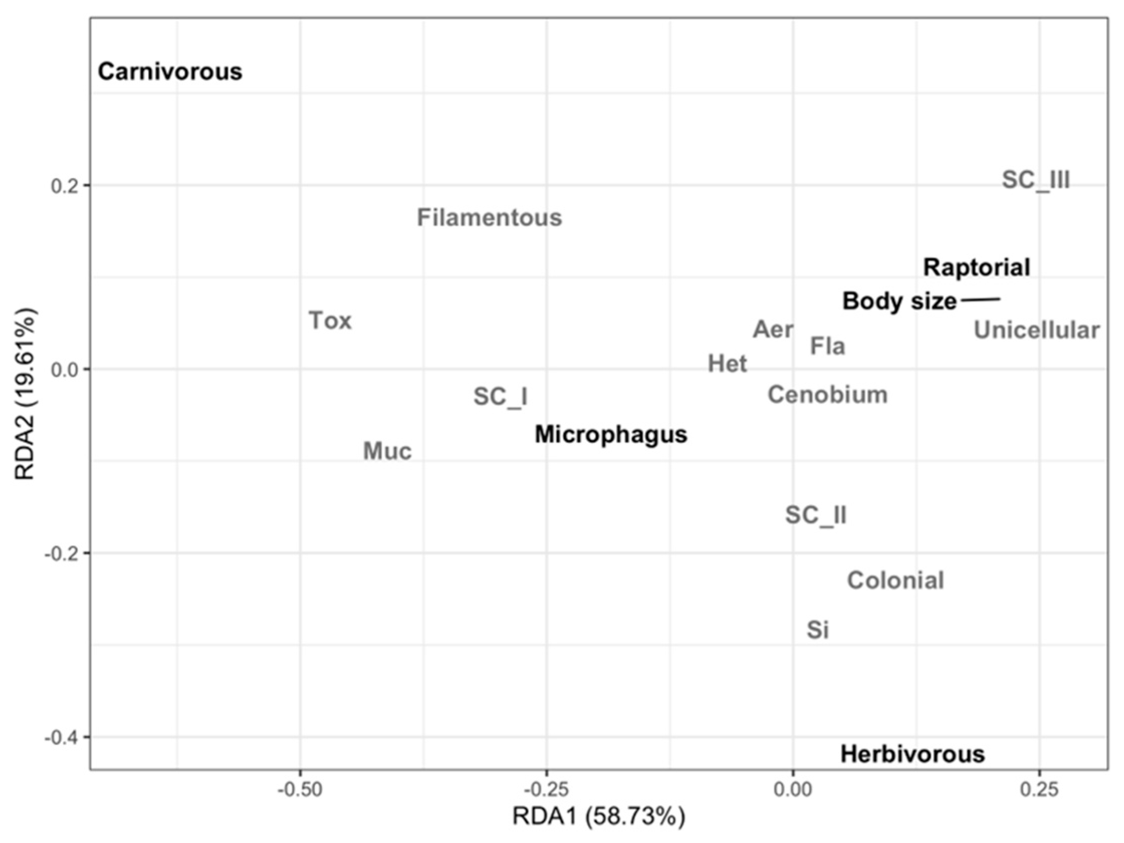
3.2. Taxonomic and Functional Diversity of the Phytoplankton Community

We identified 74 phytoplanktonic taxa, which were further assigned to six of the seven MBFGs proposed by Kruk et al., 2010 [33], namely: MBFG I (7 species), MBFG III (1 species), MBFG IV (28 species), MBFG V (18 species), MBFG VI (8 species), and MBFG VII (12 species) (Supplementary Materials Table S1). MBFGs IV, V, and VI contributed most of the phytoplankton biomass at both depths. Notably, MBFG I and VII typically had low biomass values, and MBGF III was observed only at the surface during the warmer/rainy season, with low biomass values (Figure 4).
A two-way ANOVA analysis using months and depth as fixed factors revealed a significant difference only in the total phytoplankton biomass between depths (F1 = 4.286, p < 0.05), with significantly higher biomass values at the bottom compared to the surface. Although the difference in total biomass between the months was not significant (F5 = 0.352, p > 0.05), it was possible to observe fluctuations in the biomass over time, especially in December 2017 on the surface, while at the bottom of the reservoir, the oscillation in biomass occurred in March 2018 (Figure 4). When analyzing the phytoplankton composition at each depth separately, a one-way ANOVA analysis using MBFG as a fixed factor showed a significant difference for the MBFG biomass at the surface (F5 = 11.806, p < 0.001) and the bottom (F5 = 32.778, p < 0.001) of the reservoir. The post hoc Holm–Sidak test revealed that MBFGs IV, V, and VI differed statistically from MBFGs I, III, and VII, but they did not differ from each other at ether depth. Also, this analysis showed that at the bottom of the reservoir, MBFG I was statistically different from MBFG III.
Regarding the trait–environment relationship, the first two RLQ axes explained 73.26% of the variation. Mainly, the first trait syndrome (RLQ axis 1 Trait) correlated significantly with the first environmental gradient (RLQ axis 1 Environment; r = 0.26, p < 0.01), while the second trait syndrome (RLQ axis 2 Trait) correlated significantly with the second environmental gradient (RLQ axis 2 Environment; r = 0.19, p < 0.01). The results of the RLQ showed that most of the biomass-based variation in trait syndromes was related to the reservoir vertical profile and seasonality (Figure 5A,B). The first RLQ axis summarized the vertical profile, highlighting depth and water temperature as significant variables, while the second RLQ axis summarized the temporal gradient. Specifically, the months of May and January 2018 stood out, as well as the dissolved inorganic nitrogen, pH, and zooplankton biomass (Figure 5C). Notably, the spatial and temporal distribution of environmental conditions coupled with the biomass and distribution of MBFG was highlighted by the biomass of MBFG III during January 2018 (Figure 5B); a correlation was found between water temperature and functional traits such as aerotopes, heterocytes, and toxins in the months of January 2018 and March 2018 (Figure 5A); and the biomass of MBFG V (Figure 5B) was linked to functional traits such as the volume and flagella at the bottom of the reservoir (Figure 5A). The analysis also revealed that zooplankton was significant and was associated with the presence of flagellated phytoplankton species.

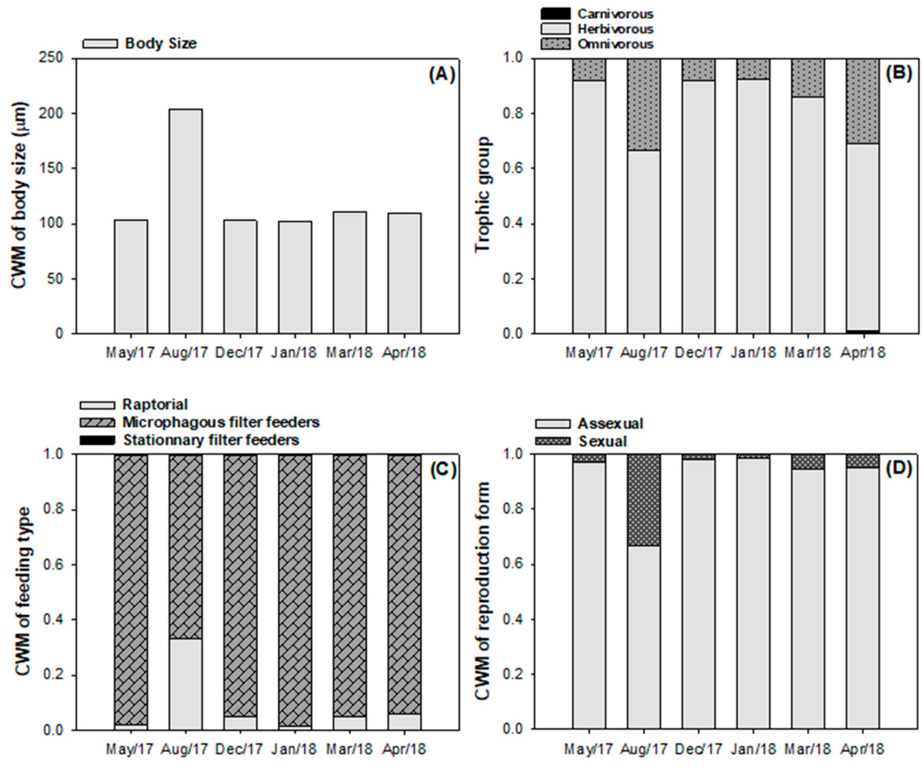
3.3. Taxonomic and Functional Diversity of Zooplankton Community

We registered two cladocerans, one cyclopoid copepod, and eight rotifer species, totaling 11 taxa (Supplementary Materials Table S2). The density of the zooplankton community varied from 0.21 ind. L−1 to 1469.43 ind. L−1, being predominantly composed of rotifers, copepods, and cladocerans, respectively (Figure 6A,B). A two-way ANOVA demonstrated that the density values were statistically different between the taxonomic groups (F2 = 28.427, p < 0.05), but the density did not change significantly across the months (F5 = 3.079, p > 0.05). The post hoc Holm–Sidak test revealed that rotifers, copepods, and cladocerans exhibited significant differences in density values, with rotifers showing the highest densities, followed by cyclopoid copepods and cladocerans (p < 0.05).
Zooplankton biomass varied from 4.25 × 10⁴ µg C L−1 to 67.34 µg C L−1. A two-way ANOVA demonstrated that the biomass between months (F5 = 4.798, p < 0.05) and between taxonomic groups (F2 = 30.509, p < 0.05) was statistically different. Regarding the sampled months, there was a significant reduction in the total biomass of the zooplankton community from May to August/2017, mainly for cyclopoid copepod biomass (p < 0.05) (Figure 6C,D). Even so, cyclopoid copepods exhibited a significantly higher biomass, contributing to >83% of the biomass during the study (Figure 6C,D). Rotifers were present in all months, but with significantly less biomass compared to cyclopoid copepods (p < 0.05), though there was no significant difference compared to cladocerans biomass (p < 0.05). Meanwhile, cladocerans were observed only in March 2017 and January 2018 (Figure 6C,D).
The CWM values of body size showed a dominance of species with small body sizes (<210 µm), predominantly herbivorous rotifers: microphagous filter-feeders with asexual reproduction (Figure 7). Other functional traits increased depending on the month. For instance, omnivorous species increased the CWM values in August 2017 and April 2018 (Figure 7B), while raptorial feeders (Figure 7C) and sexually reproducing species (Figure 7D) dominated in August 2017. These results are based on the abundance (not biomass) of the functional traits of the zooplankton community.
The CWM-RDA analysis using the functional traits of the phytoplankton and zooplankton explained 30.12% of the variation in phytoplankton trait composition based on the variations in zooplankton trait composition, from which 95.57% of the variation was captured by the first two RDA axes (axis 1 = 58.73% and axis 2 = 19.61%; Figure 8). Herbivorous zooplankton were correlated with siliceous exoskeleton phytoplankton, such as those in MBFG VI, or with colonial phytoplankton, mostly those falling within size class II (SC_II; MLD 20–50 µm). Raptorial zooplankton correlated with several functional traits of phytoplankton, such as unicellular, flagella, aerotopes, heterocytes, and coenobium life forms, mostly those falling within size class III (SC_III; MLD ≥ 50 µm). Microphagous filter feeders correlated with phytoplankton within size class I (SC_I; MLD ≤ 20 µm). Notably, herbivorous zooplankton had a negative correlation with filamentous phytoplankton and toxins that could be observed in MBFG III (Figure 8).

4. Discussion

We found that phytoplankton diversity and biomass were driven by environmental variables, leading to a prevalent contribution of MBFGs IV, V, and VI, especially during the warmer/rainy season. Thermal stratification led to the occurrence of MBFG III. These findings support our first hypothesis that abiotic factors are the main drivers of phytoplankton community dynamics. Although thermal stratification did not increase the biomass of fast-growing MBFG I or lead to the emergence of MBFG II, it did result in the appearance of MBFG III, partially confirming our second hypothesis that heterogeneous conditions promote the coexistence of different phytoplankton traits.
Regarding the zooplankton community, the total biomass remained stable over time, with cyclopoid copepods and rotifers prevailing. These zooplankton were typically small-bodied, herbivorous, microphagous filter-feeders with asexual reproduction. The CWM-RDA revealed interactions between the functional traits of the phytoplankton and zooplankton, even though the total zooplankton biomass did not correlate with the total phytoplankton biomass. Herbivorous zooplankton were associated with siliceous exoskeletal phytoplankton (MBFG VI) and colonial phytoplankton (size class II). Raptorial feeders were linked to unicellular life forms, flagella, aerotopes, heterocytes, and coenobium (size class III), while microphagous filter feeders correlated with the phytoplankton in size class I. Herbivorous zooplankton negatively correlated with filamentous phytoplankton and toxins in MBFG III. Therefore, our third hypothesis—that high functional diversity of phytoplankton would increase the niche space for zooplankton communities, leading to top-down control—was rejected.
The phytoplankton community demonstrated a vertical distribution in the total biomass and the composition of the MBFG. Although the statistical analysis did not reveal a significant difference in phytoplankton biomass between the months sampled, it was possible to observe a sharp decrease in the total biomass between January and March 2018. Notably, the precipitation during this period was above the average of the last 13 years (Sistema Alerta Rio–Rio de Janeiro, RJ, 2020), which possibly resulted in an increased wash-out rate, leading to the loss of phytoplankton species [1]. Such losses are expected to be more pronounced in environments that have a high abundance of slow-growth individuals (MBFG IV-VI) [20], such as those observed in the Camorim Reservoir. Of the prevalent MBFGs, groups IV and V can tolerate moderate to limiting resources [33]. For example, species from MBFG V can execute mixotrophic strategies, which improves their fitness under low to limiting nutrient conditions [87]. Notably, while these MBFGs provide a good food source for zooplankton [26] due to their high content of fatty acids and high-fat polyunsaturated acids (PUFAs) [88,89], their large body size can hinder their consumption, increasing their fitness under high grazing pressures. Moreover, the RDA-CWM results demonstrate a correlation between small phytoplankton (size class I) and microphagous filter feeders. This feeding type suggests lower energy costs, the ability to survive low food consumption conditions [8], and strong microbial grazing [90], which are consistent with the body size of the zooplankton community and the density of the rotifers observed in the reservoir. Therefore, the environmental conditions associated with the functional traits belonging to MBFG IV and V and the preference of zooplankton for small-bodied individuals can explain the dominance of these MBFGs in the Camorim Reservoir.
MBFG I is composed of small organisms with a high surface-to-volume ratio and fast growth rate that are adapted to the rapid acquisition of resources [33]. Interestingly, the low concentration of SRP could be a positive factor for the development of MBFG I in the Camorim Reservoir, since this group can be favored in low concentrations of nutrients due to a rapid exchange of nutrients across the cell surface [91]. However, the low biomass observed across all months can be explained by the reduced body size of the species, since the methodology used to obtain the biovolume takes into account the morphology (e.g., length and width). Another explanation for the low biomass of MBFG I is predation. Species belonging to this functional group are highly ingested, especially by rotifers [26].
Thermal stratification led to the emergence of MBFG III, while MBFG VII was observed almost every month. Previous studies have demonstrated that stratification periods can favor MBFG III and VII, allowing them to dominate the pelagic zone when environmental conditions are favorable (e.g., high temperatures, water column stability, and light availability) [4,7]. Although it was not measured in this study, shallow tropical ecosystems may not experience lasting thermal stratification, and under these conditions, cyanobacteria do not achieve a significant biomass [92]. The combination of SRP limitations and the possibility of non-lasting thermal stratification may explain the low biomass of MBFG III and VII in the Camorim Reservoir. Conversely, the period of complete mixing of the water column and availability of SRSi resulted in an increase in the biomass of MBFG VI on the surface. The availability of light in the water column explains the high abundance of MBFG VI at the bottom of the reservoir. MBFG VI consists of organisms with a siliceous skeleton [33], which provides protection against mechanical pressure [1], acts as a barrier against zooplankton grazing [2], and promotes rapid sedimentation rates [1]. Additionally, SRP limitations may have benefited MBFG VI in the reservoir, as diatoms are considered to be good competitors for phosphorus [93].
The drastic reduction in the total biomass of the zooplankton community in August 2017 may have been caused by a synergism of factors. First, August/2017 was the coldest month observed in the Camorim Reservoir, which may have affected the reproduction and development of the zooplankton. Previous studies have demonstrated that temperature is one of the main environmental variables that affect the growth, reproduction, metabolism, and food preference of zooplankton organisms [94,95,96,97,98]. Second, the increase in CWM values favors sexual reproduction by copepods, as this type of reproduction generates a smaller number of individuals per offspring. Additionally, copepods have different life stages before reaching adulthood, leading to a longer life cycle compared to rotifers and cladocerans [99]. Surprisingly, the drop in phytoplankton biomass in March 2018 did not negatively affect the biomass of the zooplankton community. This can be explained by the results of the CWM, which showed that the zooplankton organisms were small-bodied, herbivorous, omnivorous, and microphagous filter-feeders. Therefore, a community with small-bodied zooplankton, such as in the Camorim Reservoir, reduces the prey size spectrum, reflecting poor grazing on medium- to large-sized phytoplankton species. Additionally, cyclopoid copepods are highly selective organisms that are known to graze on mobile heterotrophic prey (e.g., ciliates) [32], while rotifers prefer bacteria, flagellates, and organic detritus [100]. Taken together, copepods and rotifers have similar omnivorous feeding habits, which may explain their non-exclusive dependence on phytoplankton as a food resource.
Although some studies have already linked the functional traits of zooplankton to top-down control in phytoplankton [22], our CWM-RDA demonstrating positive and negative trait interactions among phytoplankton and zooplankton is novel. Raptorial zooplankton correlated positively with unicellular flagellated phytoplankton and phytoplankton class III. Laboratory experiments indicate that MBFG V or representative species of this group (e.g., Cryptomonas sp.) are readily consumed by both cladocerans and copepods [21,26,100,101], as they are highly nutritious and serve as edible prey for zooplankton [33]. Furthermore, the size class of MBFG V in our results was classified into I and II, making them potential prey for small zooplankton. Raptorial zooplankton, such as cyclopoid copepods, can capture and kill their prey due to a complex feeding apparatus, allowing them to select their prey [37,102,103,104]. The positive correlation between raptorial zooplankton and phytoplankton with functional traits such as aerotopes, heterocytes, coenobium, and a larger body size (size class III) may be an indirect effect of cyclopoid copepods, as these organisms select more palatable prey like MBFG V. This selection reduces competition for resources and may consequently favor the development of less-palatable phytoplankton species, such as cyanobacteria.
Another key result was the positive correlation between herbivorous zooplankton and siliceous exoskeletal phytoplankton, such as those from MBFG VI, as well as with colonial phytoplankton, mainly those belonging to size class II. Cladocerans, as herbivores, have the potential to remove MBFG VI, although they are not effectively exploited as a food source [26]. Overall, colonies are reported as an anti-herbivory functional trait due to their large size or the presence of mucilage, which makes them less edible [2]. The interactions between zooplankton and colonial phytoplankton are often associated with the presence of cyanobacteria or clustering into MBFG VII [4,7,102]. However, different phytoplankton species, such as chlorophytes, are also colony-forming and serve as a food resource for zooplankton like cladocerans [105]. The dominance of the herbivorous species observed in Camorim Reservoir was related to the high abundance of rotifers, which are known to have a small prey size spectrum [106,107]. Rotifers typically exhibit passive suspension feeding behavior with lower prey selectivity [26], suggesting weak top-down control. Additionally, the small prey size of rotifers explains their negative correlation with the filamentous and toxin traits of phytoplankton, as all species with these traits were cyanobacteria. Although rotifers have demonstrated the ability to graze on filamentous species under laboratory conditions [107,108], in a natural environment with diverse prey availability, they prefer more palatable prey (e.g., smaller in size and non-filamentous).

5. Conclusions

Our results demonstrate that phytoplankton biomass and diversity are closely linked to environmental variables. The omnivorous traits present in cyclopoid copepods and some species of rotifers were crucial for maintaining zooplankton community biomass in the reservoir due to their low dependence on phytoplankton as a food source. There was a weak but significant effect of zooplankton functional diversity on phytoplankton functional diversity, mainly because of the dominance of small-body-size zooplankton. Altogether, our findings suggest that environmental filtering plays a greater role in phytoplankton community formation than the zooplankton grazing in this shallow tropical reservoir.

Supplementary Materials

The following supporting information can be downloaded at: https://www.mdpi.com/article/10.3390/d16080438/s1, Table S1—List of phytoplankton taxa and representative taxonomic groups observed in the Camorim Reservoir between 2017 and 2018; Table S2—List of zooplankton taxa and representative taxonomic groups and functional groups observed in the Camorim Reservoir between 2017 and 2018.

Author Contributions

Conception of the article—M.C.B.M., K.A.G. and M.M.M.; data description and analysis—M.C.B.M. and C.G.-R.; writing—M.C.B.M.; review and editing—C.G.-R., L.d.M., K.A.G. and M.M.M.; supervision—M.M.M. All authors have read and agreed to the published version of the manuscript.

Funding

Marcella C. B. Mesquita’s PhD scholarship was funded by Coordenação de Aperfeiçoamento de Pessoal de Nível Superior (CAPES) and by Fundação Carlos Chagas Filho de Amparo à Pesquisa do Estado do Rio de Janeiro (FAPERJ).

Data Availability Statement

The data published in this article come from Marcella C. B. Mesquita’s doctorate thesis. As there are other articles that are yet to be published from this researcher’s doctorate, the data will not yet be publicly presented. The main raw data relating to this manuscript will be available as supplementary materials.

Acknowledgments

We would like to cordially thank the members of the Phytoplankton Ecology and Physiology Laboratory (UERJ) for their technical support.

Conflicts of Interest

The authors declare no conflicts of interest.

References

  1. Reynolds, C.S. Ecology of Phytoplankton; Cambridge University Press: New York, NY, USA, 2006. [Google Scholar]
  2. Lürling, M. Grazing resistance in phytoplankton. Hidrobiologia 2021, 848, 237–249. [Google Scholar] [CrossRef]
  3. Costa, M.R.A.; Cardoso, M.M.L.; Selmeczy, G.B.; Padisák, J.; Becker, V. Phytoplankton functional responses induced by extreme hydrological events in a tropical reservoir. Hydrobiologia 2024, 851, 849–867. [Google Scholar] [CrossRef]
  4. Magalhães, L.; Rangel, L.M.; Rocha, A.M.; Cardoso, S.J.; Silva, L.H.S. Responses of morphology-based phytoplankton functional groups to spatial variation in two tropical reservoirs with long water-residence time. Inland. Waters 2020, 11, 29–43. [Google Scholar] [CrossRef]
  5. Carvalho, L. Top-down control of phytoplankton in a shallow hypertrophic lake: Little Mere (England). Hydrobiologia 1994, 275–276, 53–63. [Google Scholar] [CrossRef]
  6. Jeppesen, E.; Sondergaard, M.; Jensen, J.P.; Mortensen, E.; Sortkjaer, O. Fish-induced changes in zooplankton grazing on phytoplankton and bacterioplankton: A long-term study in shallow hypertrophic Lake Sebygaard. J. Plankton Res. 1996, 18, 1605–1625. [Google Scholar] [CrossRef]
  7. Rangel, L.M.; Soares, M.C.S.; Paiva, R.; Silva, L.H.S. Morphology-based functional groups as effective indicators of phytoplankton dynamics in a tropical cyanobacteria-dominated transitional river–reservoir system. Ecol. Indic. 2016, 64, 217–227. [Google Scholar] [CrossRef]
  8. Josué, I.I.P.; Cardoso, S.J.; Miranda, M.; Mucci, M.; Ali, K.G.; Roland, F.; Marinho, M.M. Cyanobacteria dominance drives zooplankton functional dispersion. Hydrobiologia 2019, 831, 149–161. [Google Scholar] [CrossRef]
  9. Heathcote, A.J.; Filstrup, C.T.; Kendall, D.; Downing, J.A. Biomass pyramids in lake plankton: Influence of cyanobacteria size and abundance. Inland. Waters 2016, 6, 250–257. [Google Scholar] [CrossRef]
  10. Krztoń, W.; Kosiba, J.; Pociecha, A.; Wilk-Woźniak, E. The effect of cyanobacterial blooms on bio- and functional diversity of zooplankton communities. Biodivers. Conserv. 2019, 28, 815–1835. [Google Scholar] [CrossRef]
  11. Krztoń, W.; Kosiba, J. Variations in zooplankton functional groups density in freshwater ecosystems exposed to cyanobacterial blooms. Sci. Total Environ. 2020, 730. [Google Scholar] [CrossRef] [PubMed]
  12. Costa, M.R.A.; Attayde, J.L.; Becker, V. Effects of water level reduction on the dynamics of phytoplankton functional groups in tropical semi-arid shallow lakes. Hydrobiologia 2016, 778, 75–89. [Google Scholar] [CrossRef]
  13. Dalu, T.; Wasserman, R.J. Cyanobacteria dynamics in a small tropical reservoir: Understanding spatio-temporal variability and influence of environmental variables. Sci. Total Environ. 2018, 643, 835–841. [Google Scholar] [CrossRef] [PubMed]
  14. Mesquita, M.C.B.; Lürling, M.; Door, F.; Pinto, E.; Marinho, M.M. Combined effect of light and temperature on the production of saxitoxins in Cylindrospermopsis raciborskii strains. Toxins 2019, 11, 38. [Google Scholar] [CrossRef]
  15. Mesquita, M.C.B.; Prestes, A.C.C.; Gomes, A.M.A.; Marinho, M.M. Direct effects of temperature on growth of different tropical phytoplankton species. Microb. Ecol. 2020, 79, 1–11. [Google Scholar] [CrossRef]
  16. Barbosa, L.G.; Barbosa, F.A.R.; Bicudo, C.E.M. Is thermal stability a factor that influences environmental heterogeneity and phytoplankton distribution in tropical lakes? Acta Limnol. 2018, 30. [Google Scholar] [CrossRef]
  17. Longhi, M.L.; Beinser, B.E. Patterns in taxonomic and functional diversity of Lake Phytoplankton. Freshw. Biol. 2010, 55, 1349–1366. [Google Scholar] [CrossRef]
  18. Rangel, L.M.; Silva, L.H.S.; Rosa, P.; Roland, F.; Huszar, V.L.M. Phytoplankton biomass is mainly controlled by hydrology and phosphorus concentrations in tropical hydroelectric reservoirs. Hydrobiologia 2012, 693, 3–28. [Google Scholar] [CrossRef]
  19. Reynolds, C.S. Vegetation Processes in the Pelagic: A Model for Ecosystem Theory; Ecology Institute: Oldendorf, Germany, 1997. [Google Scholar]
  20. Scheffer, M. Ecology of Shallow Lakes; Kluwer Academic Publishers: Dordrecht, The Netherlands, 1998; 357p. [Google Scholar]
  21. Leitão, E.; Ger, K.A.; Panosso, R. Selective grazing by a tropical copepod (Notodiaptomus iheringi) facilitates Microcystis dominance. Front. Microbiol. 2018, 9, 301. [Google Scholar] [CrossRef]
  22. Leitão, E.; Panosso, R.; Molica, R.; Ger, K.A. Top-down regulation of filamentous cyanobacteria varies among a raptorial versus current feeding copepod across multiple prey generations. Freshw. Biol. 2020, 66, 142–156. [Google Scholar] [CrossRef]
  23. Severiano, J.S.; Almeida-Melo, V.L.S.; Bittencourt-Oliveira, M.C.; Chia, M.A.; Moura, A.N. Effects of increased zooplankton biomass on phytoplankton and cyanotoxins: A tropical mesocosm study. Harmful Algae 2018, 71, 10–18. [Google Scholar] [CrossRef] [PubMed]
  24. Faithfull, C.; Goetze, E. Copepod nauplii use phosphorus from bacteria, creating a short circuit in the microbial loop. Ecol. Lett. 2019, 22, 1462–1471. [Google Scholar] [CrossRef]
  25. Jagadeesan, L.; Jyothibabu, R.; Arunpandi, N.; Anjusha, A.; Parthasarathi, S.; Pandiyarajan, R.S. Feeding preference and daily ration of 12 dominant copepods on mono and mixed diets of phytoplankton, rotifers, and detritus in a tropical coastal water. Environ. Monit. Assess. 2017, 189, 503. [Google Scholar] [CrossRef]
  26. Colina, M.; Calliari, D.; Carballo, C.; Kruk, C. A trait-based approach to summarize zooplankton– phytoplankton interactions in freshwaters. Hydrobiologia 2016, 767, 221–233. [Google Scholar] [CrossRef]
  27. Sommer, U.; Sommer, F.; Santer, B.; Jamieson, C.; Boersma, M.; Becker, C.; Hansen, T. Complementary impact of copepods and cladocerans on phytoplankton. Ecol. Lett. 2001, 4, 545–550. [Google Scholar] [CrossRef]
  28. Sommer, U.; Soomer, F. Cladocerans versus copepods: The cause of contrasting top–down controls on freshwater and marine phytoplankton. Oecologia 2006, 147, 183–194. [Google Scholar] [CrossRef]
  29. Rangel, L.M.; Silva, L.H.S.; Faassen, E.J.; Lürling, M.; Ger, K.A. Copepod prey selection and grazing efficiency mediated by chemical and morphological defensive traits of cyanobacteria. Toxins 2020, 12, 465. [Google Scholar] [CrossRef]
  30. Amorim, C.H.; Valença, C.R.; Moura-Falcão, R.H.; Moura, A.N. Seasonal variations of morpho-functional phytoplankton groups influence the top-down control of a cladoceran in a tropical hypereutrophic lake. Aquat. Ecol. 2019, 53, 453–464. [Google Scholar] [CrossRef]
  31. Severiano, J.S.; Amaral, C.B.; Diniz, A.S.; Moira, A.N. Species-specific response of phytoplankton to zooplankton grazing in tropical eutrophic reservoirs. Acta Limnol. 2021, 33. [Google Scholar] [CrossRef]
  32. Kiørboe, T. How zooplankton feed: Mechanisms, traits and trade-offs. Biol. Rev. 2011, 86, 311–339. [Google Scholar] [CrossRef]
  33. Kruk, C.; Huszar, V.L.M.; Peeters, E.T.H.; Bonilla, S.; Costa, L.; Lürling, M.; Reynolds, C.S.; Scheffer, M. A morphological classification capturing functional variation in phytoplankton. Freshw. Biol. 2010, 55, 614–627. [Google Scholar] [CrossRef]
  34. Litchman, E.; Ohman, M.D.; Kiørboe, T. Trait-based approaches to zooplankton communities. J. Plankton Res. 2013, 35, 473–484. [Google Scholar] [CrossRef]
  35. Violle, C.; Navas, M.; Vile, D.; Kazakou, E.; Fortunel, C.; Hummel, I.; Garnier, E. Let the concept of trait be functional! Oikos 2007, 116, 882–892. [Google Scholar] [CrossRef]
  36. Cadotte, M.W.; Carscadden, K.; Mirotchnick, N. Beyond species: Functional diversity and the maintenance of ecological processes and services. J. App Ecol. 2011, 48, 1079–1087. [Google Scholar] [CrossRef]
  37. Barnett, A.J.; Finlay, K.; Beisner, B.E. Functional diversity of crustacean zooplankton communities: Towards a trait-based classification. Freshw. Biol. 2007, 52, 796–813. [Google Scholar] [CrossRef]
  38. Graco-Roza, C.; Soinine, J.; Corrêa, G.; Pacheco, F.S.; Miranda, M.; Domingos, P.; Marinho, M.M. Functional rather than taxonomic diversity reveals changes in the phytoplankton community of a large dammed river. Ecol. Indic. 2021, 121, 107048. [Google Scholar] [CrossRef]
  39. Inepac (Instituto Estadual do Patrimônio Cultural). Inventário de identificação dos reservatórios da CEDAE. Levantado por M.G. Ferraz, M.G. Mendonça e Rui Veloso (1998) e Iracema Franco (2006). Secretaria de Estado de Cultura, RJ. Available online: https://www.ipatrimonio.org/wp-content/uploads/2019/08/ipatrimonio-Rio-de-Janeiro-Reservatorio-Livramento-Fonte-Inepac-compactado.pdf (accessed on 12 April 2023).
  40. Menezes, M. New species of pigmented flagellates from southeastern Brazil. Arch. Protistenkd. 1996, 147, 101–105. [Google Scholar] [CrossRef]
  41. Menezes, M.; Bicudo, C.E.M. Flagellate green algae from four water bodies in the state of Rio de Janeiro, Southeast Brazil. Hoehnea 2008, 35, 435–468. [Google Scholar] [CrossRef]
  42. Pereira, U.J. Regulação do Fitoplâncton, Dinâmica Trófica Pelágica e Abordagem Experimental Aplicada ao Biocontrole de Cylindrospermopsis raciborskii em Reservatório Eutrófico Tropical (Reservatório do Camorim, Parque Estadual da Pedra Branca, RJ). Ph.D. Thesis, Federal University of Rio de Janeiro, Rio de Janeiro, Brazil, 2018. [Google Scholar]
  43. Cole, G.A. Textbook of Limnology; Waveland Press Inc.: Long Grove, IL, USA, 1994. [Google Scholar]
  44. Padisák, J.; Barbosa, F.; Koschel, R.; Krienitz, L. Deep layer cyanoprokaryota maxima in temperate and tropical lakes. Arch. Hydrobiol. Spec. Issues Advanc. Limnol. 2003, 58, 175–199. [Google Scholar]
  45. Sas, H. Lake Restoration by Reduction of Nutrient Loading: Expectations, Experiences, Extrapolations; Academia Verlag Richarz: St. Augustin, FL, USA, 1989. [Google Scholar]
  46. Uhelinger, V. Étude statistique des méthodes de dénobrement planctonique. Arch. Sci. 1964, 17, 121–123. [Google Scholar]
  47. Utermöhl, H. Zur Vervollkommnung der quantitativen Phytoplankton-Methodik: Mit 1 Tabelle und 15 abbildungen im Text und auf 1 Tafel. Int. Ver. Theor. Angew. Limnol. Mitteilungen 1958, 9, 1–38. [Google Scholar] [CrossRef]
  48. Lund, J.W.G.; Klipling, C.; Le Cren, E.D. The inverted microscope method of estimating algal numbers and the statistical basis of estimating by counting. Hydrobiologia 1958, 11, 143–170. [Google Scholar] [CrossRef]
  49. Hoek, C.V.D.; Mann, D.G.; Jahns, H.M. Algae: An Introduction to Phycology; Cambridge University Press: New York, NY, USA, 1995. [Google Scholar]
  50. Round, F.E.; Crawford, R.M.; Mann, D.G. The Diatoms. Biology and Morphology of Genera; Cambridge University Press: Cambridge, UK, 1990. [Google Scholar]
  51. Komárek, J.; Anagnostidis, K. Cyanoprokaryota I. Teil Chroococcales; Ettl, H., Gärtner, G., Heynig, H., Mollenhauer, D., Eds.; Süsswasserflora von Mitteleuropa; Gustav Fischer Verlag: Jena, Germany, 1999. [Google Scholar]
  52. Komárek, J.; Anagnostidis, K. Cyanoprokaryota 2. Teil Oscillatoriales. Büdel, B., Krienitz, L., Gärtner, G., Schagerl, M., Eds.; Süsswasserflora von Mitteleuropa; Gustav Fischer Verlag: Jena, Germany, 2005. [Google Scholar]
  53. Hillebrand, H.; Dürseken, D.; Kirschiel, D.; Pollingher, U.; Zohary, T. Biovolume calculation for pelagic and benthic microalgae. J. Phycol. 1999, 35, 403–424. [Google Scholar] [CrossRef]
  54. Carpenter, E.J.; Subramaniam, A.; Capone, D.G. Biomass and primary productivity of the cyanobacterium Trichodesmium spp. in the tropical N Atlantic Ocean. Deep-Sea Res. 2004, 51, 173–203. [Google Scholar] [CrossRef]
  55. Menden-Deuer, S.; Lessard, E.J. Carbon to volume relationships for dinnoflagellates, diatoms, and other protist plankton. L&O 2000, 4, 569–579. [Google Scholar]
  56. Montagnes, D.J.S.; Franklim, D.J. Effect of temperature on diatom volume, growth rate, and carbon and nitrogen content: Reconsidering some paradigms. L&O 2001, 46, 2008–2018. [Google Scholar]
  57. Verity, P.G.; Robertson, C.; Tronzo, C.R.; Andrews, M.G.; Nelson, J.R.; Sieracki, M.E. Relationships between cell volume and the carbon and nitrogen content of marine photosynthetic nanoplankton. L&O 1992, 37, 1434–1446. [Google Scholar]
  58. Prepas, E.E. Some statistical methods for the design of experiments and analysis of samples. In A Manual on Methods for the Assessment of Secondary Productivity in Fresh Waters, 2nd ed.; Downing, J.A., Rigler, F.H., Eds.; Blackwell Scientific Publications: Oxford, UK, 1984; pp. 266–335. [Google Scholar]
  59. Ruttner-Kolisko, A. Suggestions for biomass calculation of plankton rotifers. Arch. Hydrobiol. 1977, 8, 71–76. [Google Scholar]
  60. Mccauley, E. The estimation of the abundance and biomass of zooplankton in samples. In A Manual on Methods for the Assessment of Secondary Productivity in Fresh Waters, 2nd ed.; Dowing, J.A., Rigler, F.H., Eds.; Blackwell Scientific Publications: Oxford, UK, 1984; pp. 228–264. [Google Scholar]
  61. Bottrell, H.H.; Duncan, A.; Gliwicz, Z.M.; Grygierek, E.; Herzig, A.; Hillbrichtilkowska, A.; Kurasawa, H.; Larsson, P.; Weglenska, T. Are view of some problems in zooplankton production studies. Nor. J. Zool. 1976, 24, 419–456. [Google Scholar]
  62. Pace, M.L.; Orcutt, J.D. The relative importance of protozoans, rotifers, and crustaceans in a freshwater zooplankton community. L&O 1981, 26, 822–830. [Google Scholar]
  63. Idris, B.A.G.; Fernando, C.H. Two new species of cladoceran crustaceans of the genera Macrothrix baird and Alona baird from Malaysia. Hydrobiologia 1981, 76, 8–85. [Google Scholar] [CrossRef]
  64. Masundire, H.M. Mean individual dry weight and length-weight regressions of some zooplankton of Lake Kariba. Hydrobiologia 1994, 272, 231–238. [Google Scholar] [CrossRef]
  65. Matsumura-Tundisi, T.; Rietzler, A.C.; Tundisi, J.G. Biomass (dry weight and carbon content) of plankton crustacea from Broa reservoir (Sao Carlos, S.P.-Brazil) and its fluctuation across one year. Hydrobiologia 1989, 179, 229–236. [Google Scholar] [CrossRef]
  66. Panarelli, E.A.; Casanova, S.M.C.; Henry, R. Secondary production and biomass of Cladocera in marginal lakes after the recovery of their hydrologic connectivity in a river–reservoir transition zone. L&O Res. Manag. 2010, 15, 319–334. [Google Scholar]
  67. Culver, D.A.; Boucherle, M.M.; Bean, D.J.; Fletcher, J.W. Biomass of freshwater crustacean zooplankton from length-weight regressions. Can. J. Fish. Aquat. Sci. 1985, 42, 1380–1390. [Google Scholar] [CrossRef]
  68. Burns, C.W. Relation between filtering rate, temperature and body size in four species of Daphnia. L&O 1969, 14, 693–700. [Google Scholar]
  69. Edmondson, W.T.; Winberg, G.G. A Manual on Methods for the Assessment of Secondary Productivity in Fresh Waters; IBP Handbook No. 17; Blackwell: Oxford, UK, 1971; p. 358. [Google Scholar]
  70. Hessen, D.O. Factors determining the nutritive status and production of zooplankton in a humic lake. J. Plankton Res. 1989, 11, 649–664. [Google Scholar] [CrossRef]
  71. Persson, G.; Ekbohm, G. Estimation of dry weight in zooplankton populations: Methods applied to crustacean populations from lakes in the Kuokkel Area, Northern Sweden. Arch. Hydrobiol. 1980, 59, 225–246. [Google Scholar]
  72. Rosen, R.H. Length-dry weight relationships of some freshwater zooplankton. J. Freshw. Ecol. 1981, 1, 225–229. [Google Scholar] [CrossRef]
  73. Latja, R.; Salomen, K. Carbon analysis for determination of individual biomasses of planktonic animals. Verh. Internat Verein Limnol. 1978, 20, 2556–2560. [Google Scholar] [CrossRef]
  74. Lokko, K.; Virro, T.; Kotta, J. Seasonal variability in the structure and functional diversity of psammic rotifer communities: Role of environmental parameters. Hydrobiologia 2017, 796, 287–307. [Google Scholar] [CrossRef]
  75. Obertegger, U.; Smith, H.A.; Flaim, G.; Wallace, R.L. Using the guild ratio to characterize pelagic rotifer communities. Hydrobiologia 2011, 662, 157–162. [Google Scholar] [CrossRef]
  76. Dolédec, S.; Chessel, D.; Ter Braak, C.J.F.; Champely, S. Matching species traits to environmental variables: A new three-table ordination method. Environ. Ecol. Stat. 1996, 3, 143–166. [Google Scholar] [CrossRef]
  77. Dray, S.; Choler, P.; Dolédec, S.; Peres-Neto, P.R.; Thuiller, W.; Pavoine, S.; Ter Braak, C.J.F. Combining the fourth-corner and the RLQ methods for assessing trait responses to environmental variation. Ecology 2014, 95, 14–21. [Google Scholar] [CrossRef]
  78. Legendre, P.; Galzin, R.; Harmelin-Vivien, M.L. Relating behavior to habitat: Solutions to the fourth-corner problem. Ecology 1997, 78, 547–562. [Google Scholar] [CrossRef]
  79. Dray, S.; Dufour, A.B. The ade4 package: Implementing the duality diagram for ecologists. J. Stat. Softw. 2007, 22, 1–20. [Google Scholar] [CrossRef]
  80. Ricotta, C.; Moretti, M. CWM and Rao’s quadratic diversity: A unified framework for functional ecology. Oecologia 2011, 167, 181–188. [Google Scholar] [CrossRef]
  81. Pla, L.; Casanoves, F.; Di Rienzo, J. Quantifying Functional Biodiversity; Springer: Dordrecht, The Netherlands, 2011. [Google Scholar]
  82. Laliberté, E.; Legendre, P. A distance-based frameworkfor measuring functional diversity from multiple traits. Ecology 2010, 91, 299–305. [Google Scholar] [CrossRef]
  83. Laliberté, E.; Legendre, P.; Shipley, B. FD: Measuring Functional Diversity from Multiple Traits, and Other Tools for Functional Ecology. R Package Version 1. 2014, 0–12. Available online: https://citeseerx.ist.psu.edu/document?repid=rep1&type=pdf&doi=c0123be0f0737359fa9303aece03fd500d2499b1 (accessed on 25 May 2024).
  84. Kleyer, M.; Dray, S.; Bello, F.; Leps, J.; Pakeman, R.J.; Strauss, B.; Thuiller, W.; Lavorel, S. Assessing species and community functional responses to environmental gradients: Which multivariate methods? J. Veg. Sci. 2012, 23, 805–821. [Google Scholar] [CrossRef]
  85. Rangel, L.M.; Silva, L.H.S.; Arcifa, M.S.; Perticarrari, A. Driving forces of the diel distribution of phytoplankton functional groups in a shallow tropical lake (Lake Monte Alegre, Southeast Brazil). Braz. J. Biol. 2009, 69, 75–85. [Google Scholar] [CrossRef] [PubMed]
  86. Garnier, E.; Lavorel, S.; Ansquer, P.; Castro, H.; Cruz, P.; Dolezal, J.; Eriksson, O.; Fortunel, C.; Grigulis, K. Assessing the effects of land-use change on plant traits, communities and ecosystem functioning in grasslands: A standardized methodology and lessons from an application to 11 European sites. Ann. Bot. 2007, 99, 967–985. [Google Scholar] [CrossRef] [PubMed]
  87. Bergström, A.N.; Jansson, M.; Drakare, S.; Blomqvist, P. Occurrence of mixotrophic flagellates in relation to bacterioplankton production, light regime and availability of inorganic nutrients in unproductive lakes with differing humic contents. Freshw. Biol. 2003, 48, 868–877. [Google Scholar] [CrossRef]
  88. Ahlgren, G.; Lundstedt, L.; Brett, M.; Forsberg, C. Lipid composition and food quality of some freshwater phytoplankton for cladoceran zooplankters. J. Plankton Res. 1990, 12, 809–818. [Google Scholar] [CrossRef]
  89. Boersma, M. The nutritional quality of P-limited algae for Daphnia. L&O 2000, 45, 1157–1161. [Google Scholar]
  90. Gasol, J.M.; Duarte, C.M. Comparative analyses in aquatic microbial ecology: How far do they go? FEMS Microbiol. Ecol. 2000, 31, 99–106. [Google Scholar] [CrossRef] [PubMed]
  91. Litchman, E.; Klausmeier, C.A. Trait-based community ecology of phytoplankton. Annu. Rev. Ecol. Evol. Syst. 2007, 39, 615–639. [Google Scholar] [CrossRef]
  92. Lopes, M.R.M.; Bicudo, C.E.M.; Ferragut, M.C. Short term spatial and temporal variation of phytoplankton in a shallow tropical oligotrophic reservoir, southeast Brazil. Hydrobiologia 2005, 542, 235–247. [Google Scholar] [CrossRef]
  93. Marinho, M.M.; Azevedo, S.M.F.O. Influence of N/P ratio on competitive abilities for nitrogen and phosphorus by Microcystis aeruginosa and Aulacoseira distans. Aquat. Ecol. 2007, 41, 525–533. [Google Scholar] [CrossRef]
  94. Boersma, M.; Mathew, K.A.; Niehoff, B.; Schoo, K.L.; Franco-Santos, R.M.; Meunier, C.L. Temperature driven changes in the diet preference of omnivorous copepods: No more meat when it’s hot? Ecol. Lett. 2016, 19, 45–53. [Google Scholar] [CrossRef] [PubMed]
  95. Gusha, M.N.C.; Dalu, T.; Wasserman, R.J.; McQuaid, C.D. Zooplankton grazing pressure is insufficient for primary producer control under elevated warming and nutrient levels. Sci. Total Environ. 2019, 651, 410–418. [Google Scholar] [CrossRef] [PubMed]
  96. Angilletta, M.J.; Dunham, A.E. The temperature-size rule in ectotherms: Simple evolutionary explanations may not be general. Am. Nat. 2003, 162, 332–342. [Google Scholar] [CrossRef]
  97. Havens, K.E.; Pinto-Coelho, R.M.; Beklioğlu, M.; Christoffersen, K.S.; Jeppsen, R.; Lauridsen, T.L.; Mazumde, A.; Méthot, G.; Alloul, B.P.; Tavşanoğlu, U.N.; et al. Temperature effects on body size of freshwater crustacean zooplankton from Greenland to the tropics. Hydrobiologia 2015, 743, 27–35. [Google Scholar] [CrossRef]
  98. Burns, C.W. The relationship between body size of filter-feeding Cladocera and the maximum size of particle ingested. L&O 1968, 13, 675–678. [Google Scholar]
  99. Lenz, J. Introduction. In Zooplankton Methodology Manual; Harris, R.P., Wiebe, P.H., Lenz, J., Skjoidal, H.R., Huntley, M., Eds.; Academic Press: San Diego, CA, USA, 2000. [Google Scholar]
  100. Arndt, H. Rotifers as predators on components of the microbial web (bacteria, heterotrophic flagellates, ciliates)—A review. Hydrobiologia 1993, 255, 231–246. [Google Scholar] [CrossRef]
  101. Ger, K.A.; Leitao, E.; Panosso, R. Potential mechanisms for the tropical copepod Notodiaptomus to tolerate Microcystis toxicity. J. Plankton Res. 2016, 38, 843–854. [Google Scholar] [CrossRef]
  102. Titocci, J.; Bom, M.; Fink, P. Morpho-functional traits reveal differences in size fractionated phytoplankton communities but do not significantly affect zooplankton grazing. Microorganisms 2022, 10, 182. [Google Scholar] [CrossRef]
  103. Hansen, B. The size ratio between planktonic predators and their prey. L&O 1994, 39, 395–403. [Google Scholar]
  104. Fuchs, H.; Franks, P. Plankton community Properties determined by nutrients and size-selective feeding. Mar. Ecol. Prog. Ser. 2010, 413, 1–15. [Google Scholar] [CrossRef]
  105. Eskinazi Sant’Anna, E.M.; Maia-Barbosa, P.M.; Barbosa, F.A.R. On the natural diet of Daphnia laevis in the eutrophic Pampulha Reservoir (Belo Horizonte, Minas Gerais). Braz. J. Biol. 2002, 62, 445–452. [Google Scholar] [CrossRef]
  106. Rothhaupt, K.O. Changes of the functional responses of the rotifers Brachionus rubens and Brachionus calyciflorus with particle sizes. L&O 1990, 35, 24–32. [Google Scholar]
  107. Miracle, M.R.; Vicente, E.; Sarma, S.S.S.; Nandino, S. Planktonic rotifer feeding in hypertrophic conditions. Int. Rev. Hydrobiol. 2014, 99, 141–150. [Google Scholar] [CrossRef]
  108. Soares, M.C.S.; Lürling, M.; Huszar, V.L.M. Responses of the rotifer Brachionus calyciflorus to two tropical toxic cyanobacteria (Cylindrospermopsis raciborskii and Microcystis aeruginosa) in pure and mixed diets with green algae. J. Plankton Res. 2010, 32, 999–1008. [Google Scholar] [CrossRef]
Figure 1. Map showing on a decreasing scale (country, state, and city) the location of the Camorim Reservoir.
Diversity 16 00438 g001
Figure 2. Accumulated precipitation and average air temperature values recorded at the Barra da Tijuca weather station between 2016 and 2019. Black vertical bars are the monthly samples. Non-existent data for the months of November 2018, December 2018, and January 2019. The gray area indicates the year in which the samples were collected.
Diversity 16 00438 g002
Figure 3. Vertical profile of temperature, dissolved oxygen, pH, and water conductivity in the water column at the sampling point in the Camorim reservoir between 2017 and 2018.
Diversity 16 00438 g003
Figure 4. Temporal (months) and vertical (surface and bottom) variations in morphology-based functional groups (MBFGs) observed in the Camorim Reservoir between 2017 and 2018. (A) Biomass of MBFGs (µg C L−1) on the surface; (B) Relative contribution of biomass of MBFGs (% µg C L−1) on the surface; (C) Biomass of MBFGs (µg C L−1) at the bottom; (D) Relative contribution of biomass of MBFGs (% µg C L−1) at the bottom.
Diversity 16 00438 g004
Figure 5. Results of the (A,B) RLQ ordination and (C,D) hypothesis testing based on a fourth-corner analysis. (A) The relationships between species traits and environmental variables. (B) The distribution of species in the functional space. Each point in the ordination plot represents the position of a species modeled according to its traits on RLQ axes 1 and 2. The black lines connect the species to the centroid of its morphology-based functional groups—MBFGs. Colors represent MBFGs. (C) the relationship between environmental variables and the trait syndromes (RLQ axis trait), and (D) the correlation between species traits and the environmental gradients (RLQ axis environment). The gray boxes in (C,D) indicate significant relationships, and the values within the boxes indicate the Pearson’s R values. The values of d give the grid size. Environmental variables: SRP = soluble reactive phosphorus; DIN = dissolved inorganic nitrogen; Si = soluble reactive silica; EZ = euphotic zone; T = water temperature (°C); COND = conductivity; DO = dissolved oxygen; Zoo = zooplankton biomass. Functional traits: Aer = aerotopes; Cen = coenobium; Col = colony; Fla = flagella; Fil = filament; Het = heterocytes; MLD = maximum linear dimension; Muc = mucilage; S = surface (area); Si = siliceous exoskeletal structures; SV = surface–volume ratio; Tox = toxins; Uni = unicellular; V = volume; Zoo = zooplankton biomass.
Diversity 16 00438 g005
Figure 6. Composition of zooplankton community observed in the Camorim Reservoir between 2017 and 2018. (A) Density of mesozooplankton community (ind. L−1); (B) relative contribution of mesozooplankton density (% ind. L−1); (C) biomass of mesozooplankton community (µg C L−1); and (D) relative contribution of mesozooplankton biomass (% µg C L−1).
Diversity 16 00438 g006
Figure 7. Total community-weighted mean trait values (CWM) of the zooplankton community observed in Camorim Reservoir between 2017 and 2018. (A) Body size; (B) trophic group (carnivorous, herbivorous, and omnivorous); (C) feeding type (raptorial, microphagous filter-feeders, and stationary suspension feeders) and (D) reproduction form (asexual or sexual).
Diversity 16 00438 g007
Figure 8. CWM-RDA analysis based on the mode of feeding (microphagous, stationary, and raptorial) and trophic group (carnivorous, herbivorous, and omnivorous) of the zooplankton community and some main functional traits of phytoplankton species. Aer = aerotopes; Fla = flagella; Het = heterocytes; Muc = mucilage; Si = siliceous exoskeletal structures; Tox = toxins. Phytoplankton class of size is based on the maximum linear dimension: SC_I ≤ 20 µm; SC_II = 20–50 µm; SC_III ≥ 50 µm.
Diversity 16 00438 g008
Table 1. Morphological description and representative taxa of the seven phytoplankton morphology-based functional groups (MBFGs). Modified from Colina et al. (2016) [26].
(MBFG)DescriptRepresentative TaxaToxicityGrazing
Susceptibility
Diversity 16 00438 i001Small organisms with high surface/volumeChlorella minutissima;
Monoraphidium minutum
NoHigh
Diversity 16 00438 i002Small-flagellated organisms with siliceous exoskeletal structuresChromulina gyrans;
Dinobryon cylindricum
NoLow
Diversity 16 00438 i003Large filaments with aerotopesDolichospermum sp.;
Raphidiopsis raciborskii
YesLow
Diversity 16 00438 i004Organisms of medium size lacking specialized traitsScenedesmus acutus;
Chlorella sp.
NoHigh
Diversity 16 00438 i005Organisms of medium size lacking specialized traitsScenedesmus acutus;
Chlorella sp.
NoHigh
Diversity 16 00438 i006Non-flagellated organisms with siliceous exoskeletonsThalassiosira weissflogi;
Cyclotella sp.
NoMedium
Diversity 16 00438 i007Large mucilaginous coloniesMicrocystis aeruginosaYesLow
Table 2. Maximum depth, euphotic zone, and relative stability of the water column (RWCS) at the sampled point at Camorim Reservoir between 2017 and 2018.
MonthsMaximum Depth (m)Euphotic Zone (m)RWCS
May 20172.502.5033.95
August 20172.702.7021.93
December 20172.102.1063.62
January 20182.902.90145.59
March 20182.702.70100.70
April 20182.302.1638.89
Table 3. Minimum values (Min), maximum values (Max), median values (Med), and coefficients of variation (CV) of the abiotic variables observed in the Camorim Reservoir between 2017 and 2018.
SurfaceBottom
MinMaxMedCVMinMaxMedCV
SRP3.56.24.80.193.65.34.80.12
DIN46.7170.5103.90.4089.3236.2165.70.28
SRSi39.6836.7271.30.848.61368.2153.81.38
DIN:SRP4.436.9180.5410.753.927.90.48
Legend. Number of measurements (n = 6); Soluble reactive phosphorus (SRP), dissolved inorganic nitrogen (DIN), soluble reactive silica (SRSi), and molar ratio between dissolved inorganic nitrogen and soluble reactive phosphorus ratio (DIN:SRP). The nutrient concentrations are expressed in µg L−1.
Disclaimer/Publisher’s Note: The statements, opinions and data contained in all publications are solely those of the individual author(s) and contributor(s) and not of MDPI and/or the editor(s). MDPI and/or the editor(s) disclaim responsibility for any injury to people or property resulting from any ideas, methods, instructions or products referred to in the content.

