Abstract
Many gaps in our theoretical understanding of the variations in the diversity and structure of intertidal communities exist for the Eastern Pacific. In order to fill some of these gaps, we censused intertidal communities and compared patterns of diversity on multiple spatial scales using several measures in alpha (α) and beta (β) diversities at twenty-one sites in a cold temperate, a warm temperate and a tropical Eastern Pacific ecoregion that were unique in terms of research effort and each with distinct geographic features. Diversity and richness on all spatial scales were compared using area curves, Hill numbers, ordination and cluster analyses, and the Hutcheson’s t-test with post hoc PERMANOVA, which revealed significant differences in diversity within and among ecoregions. Functional group and species richness and abundance were found to be highest in the cold and warm temperate ecoregions, and the functional group richness was second highest in the tropical Guayaquil ecoregion. The Bray–Curtis similarity method proved useful for determining patterns of small-scale intertidal zonation, while the Sorensen–Dice method suggested high indices of similarity in the functional group and subclass structures among all ecoregions.
1. Introduction
Rocky intertidal ecosystems provide a unique opportunity to investigate species richness and the diversity of the composition of the communities at the marine/terrestrial interface, as well as the range and spread of native and invasive species across broad regional scales. Research in this ecosystem has focused primarily on describing latitudinal gradients of abundance and diversity on relatively local scales with some comparisons made across broader regional scales. The use of diversity measures served to delineate changes in the abundance of species and range shifts following El Niño along the northern Peruvian coast [1,2] and trans-regional richness and similarities among taxonomic groups in South Africa, Chile [3,4], south-central Alaska [5], and the temperate western coast of Japan [6]. Factors driving intertidal community regulation and diversity have been synthesized from reviews of the existing literature (New Zealand, South Africa, New England, and Oregon) [7,8]. A trans-regional census of Pacific rocky intertidal communities is a prelude to not only understanding adaptations and resilience in conspecifics from dissimilar environments but the magnitude of species invasions and the effects on the thermal tolerances of foundation species to climate change as well.
Richness in the functional structures of intertidal communities has been found to be lower in ecosystems that are subject to perturbations in the environment [9] resulting from pollution, increases in the strength and frequency of El Niño, and marine heatwaves resulting from climate change. Following the Exxon Valdez oil spill in Prince William Sound, in 1987, there was considerable difficulty in assessing the damage because so little was known about the hierarchical structures and the algal biomass of the intertidal communities throughout the Sound before the spill occurred. As a result of this, a coordinated effort to understand changes in poorly studied rocky intertidal communities following catastrophic events along the eastern north Pacific coast was implemented by the United States Bureau of Oceans Management’s Multi-Agency Rocky Intertidal Network (MARINe) using a developed set of protocols to comprehensively survey multiple regions of the northeastern Pacific from Washington to Baja California. The Census data obtained from similar surveys is used to define the structure of the biological communities for any region under study, which, in turn, aids in the cause-and-effect assessment of damage following catastrophic events [10,11,12,13,14,15]. Southeast Alaska and Peru are regions of the Eastern Pacific that share similar taxa in their intertidal zones, yet the underlying similarities in species composition and functional structures are poorly understood [16]. Furthermore, both regions face immediate threats from oil spills and climate change. In this study, we use derivations of the MARINe protocols to perform a comprehensive broad-scale census of rocky intertidal communities in temperate and tropical marine ecoregions of Southeast Alaska, Chile, and Peru.
Measures of species diversity and richness from sample-based data are an effective means for describing poorly or unstudied ecosystems on multiple scales and have been universally prescribed in the scientific analysis to quantify the characteristics of community compositions. Our objectives are to analyze patterns of diversity among the communities using multiple measures of alpha diversity on multiple spatial scales; characterize the communities by describing species and functional group structures for all ecoregions; and compare species turnover on multiple spatial scales using the appropriate methods in beta diversity. We expect to find a bimodal pattern of alpha diversity, with higher species richness in the temperate regions and similar patterns in functional group richness among the ecoregions.
2. Materials and Methods
2.1. Study Sites
Each bioregional area sampled is referred to by the appropriate ecoregional name or abbreviation in accordance with Spalding et al. [17]. The ecoregions are the Guayaquil ecoregion (GUAY) in the Tropical East Pacific Province of Peru and Ecuador, the Humboldtian ecoregion in the Warm Temperate Southeast Pacific Province of Peru and Chile, which is divided here into two sub-ecoregions to provide a higher resolution of diversity based on the proximity of the shoreline to an upwelling [18], as follows: the Humboldtian Wide-Shelf (HWS), the Humboldtian Narrow-Shelf (HNS), and the North American Pacific Fjordland (NAPF) ecoregions (Figure 1). A minimum of three sites per ecoregion were established based on appropriate and accessible rocky intertidal habitat located away from major urban centers following the methodology of Wilbur et al. [16] (Table 1). Sites in the GUAY, HWS, and HNS were sampled in the austral summer of 2017, and sites in the NAPF were sampled during the boreal summers of 2015 and 2017. The highest point in the intertidal zone where algae, barnacles, or gastropods were first encountered was determined to be the highest point on the transect and where the exposure time to air is greatest and submersion time to seawater the least. One to two study plots per site measuring 10 horizontal meters by a maximum of 10 m vertical to the shoreline were established at each site by installing permanent stainless-steel bolts when a hard rock substrate was available; the bolts were anchored by drilling a 5 mm hole into the rock at the upper boundary of the plots using an impact drill and cemented in place with marine-grade epoxy. Sampling was carried out during ebb tides (between 0 and 1.0 m for the warm temperate and tropical ecoregions, and between −0.90 m mean low water (MLW) and +3 m MLW for the cold temperate ecoregion). A minimum of five transects perpendicular to the waterline spaced one to two meters apart were established using fiberglass reel tapes starting from the height where the marker bolts were installed.

Figure 1.
Map of the Eastern Pacific ecoregions where intertidal communities were sampled in this study. See Table 1 for list of ecoregion and site names and geographic coordinates.

Table 1.
Ecoregions with abbreviations (bold type), followed by sites and abbreviations, with latitude and longitude coordinates for the intertidal communities censused in this study.
2.2. Sample-Based Incidence and Abundance Scoring
Starting from the top of the transect where intertidal biota were first encountered and finishing at the waterline, invertebrates and algae were identified in increments of 10 cm in accordance with the methods used in Engle [10]. For example, on a horizontal transect of 10 m in length, the first point was scored at the 0 cm mark, and subsequent points were scored every 10 cm. To detect the incidence of species in the area surrounding each point, biota were scored within a radius that was half the distance between points on the transect (i.e., near-neighbor design). At sites with irregular substrates or where hazardous swells made conditions impossible to score along, continuous transects of a 75 cm × 50 cm strung quadrat was used for scoring. Near-neighbor species that were located around the point within a radius that was one-half the distance between points were also scored. All organisms were identified to family, genus, species, or functional taxa. Start and end times and tidal ranges were recorded for each day of sampling. The presence of sand, rock, and tidepool substrate was noted during the surveys. Taxa were photographed along the transects when possible using a Ricoh WG-4 16 mp camera attached to a 1″ diameter PVC frame that with a 50 cm × 75 cm quadrat mounted on the bottom of the framer [10]. The camera was also used to collect GPS coordinates for each site.
Abundance counts of mobile and motile invertebrates are important to include in a regional census because they are designed to capture species that inhabit specific niches that might otherwise be missed and are used to determine changes in the population over time (the term “abundance” as used in this section and in the Supplementary Material refers to the abundance of species, and all other references to the term abundance are used in the context of the statistical algorithms for measuring diversity). Such a temporal abundance survey is beyond the scope of this study; therefore, our results from the diversity analysis and niche assessments are mentioned in more detail at the end of the Supplemental Materials (Figures S27 and S28, Tables S38–S40). Mobile macrofauna such as echinoderms (sea stars and sea cucumbers) were counted for abundance inside of a 20 m × 20 m area at each site, and smaller motile species such as limpets and snails were counted for abundance using a 20 cm × 20 cm quadrat in order to capture species; these data were not added to the sample-based incidence data scored from the transects to avoid potential bias. We identified the following niche habitats where species that were found in the abundance surveys: rock crevices, effective shoreline (i.e., where a waves first wets the shore), emergent shoreline, shallow subtidal zone, tidepools, and epibionts.
Invertebrates and algae ≥ 1 mm were examined using a hand lens and a 20× Nikon field microscope and identified to species or the lowest taxonomic level using published work and reference manuals specific to each ecoregion [19,20,21]. Resources from the Instituto del Mar del Perú (IMARPE) were also used [22], as well as dichotomous keys [23,24,25]. Cryptic species of algae were collected in sterile containers and sent to PELD ILOC Universidade Federal Fluminense Niteró, Brazil, for sequencing of the UPA markers. All specimens were checked for taxonomic synonyms and accuracy by cross-referencing with Algaebase [26]. Species were then assigned to their corresponding taxonomic groups (invertebrates) and functional groups (algae) according to the methods used by Steneck et al. [9,27,28,29] for defining patterns of broad regional scale diversity.
2.3. Spatial Scales and Measures of Diversity
The treatment of the data for spatial scaling followed that of Okuda et al. [6], and it compared alpha diversity α and beta diversity β within sites, within ecoregions, and among ecoregions. On the smallest spatial scale (α1), each transect from each site was treated as a sample and used to compute the various alpha diversity indices, which were rarefied in EstimateS v.9.1.0. to compute the cumulative site alpha diversity indices for medium spatial scale (α2) comparisons of sites within the same ecoregion. The samples were also used to compute beta diversity (β1 species turnover) to determine patterns of intertidal zonation. On the medium spatial scale (β2), sites within the same ecoregion were treated as samples and analyzed for species turnover for comparison among sites within ecoregions, and large spatial scale (α3 and β3) sites within ecoregions were pooled and treated as samples for comparisons of richness, diversity, and functional group/taxonomic turnover among ecoregions. A matrix of distances between sites within and among ecoregions can be found in the Supplementary Material Table S1.
The analysis of functional and taxonomic richness for abundance data using rarefied accumulation curves similar to methods used for species area curves has been proposed as an effective method for describing diversity among regions on multiple scales, particularly when imbalances in sampling efforts exist [30]. Rarefied and extrapolated accumulation curves for sample size versus species richness (S), estimated species richness (Sest), Chao 2 richness, and functional group richness along with rarefied accumulation curves for sample size versus species diversity [31,32] were plotted for comparisons of the regional scales α2 and α3.. The Shannon–Wiener indices were analyzed for significance of variance on the scales α2 and α3 using the Hutcheson’s two-sided t-test in the ecolTest v.0.0.1 package [33].
To determine patterns of zonation on small (β1) scales, the vertical transects were stratified, pooled, and analyzed for turnover using a Bray–Curtis dissimilarity measure (at sites with irregular substrates where 70 cm × 50 cm quadrats were used, patterns of zonation were not determined). Zones were assigned starting with the highest points on the transects. A Bray–Curtis index value of <0.6 (near to or less than 50% similarity) was interpreted as species turnover, and the next section of the transect was assigned to the next appropriate lower zone, and so on. Medium scale (β2) beta diversity was analyzed for species turnover among sites within the same ecoregion by ordinating each site’s zone as a cluster group in the nMDS and cluster dendrograms. Species turnover on a large scale (β3) was analyzed by pooling the taxonomic and functional group data for each ecoregion (GUAY, HWS, HNS, and NAPF).
We employed various measures of diversity to delineate areas of species turnover, to identify areas of species abundance, and to detect the probability of a single given species and alterations to the community composition on multiple spatial scales [34,35,36,37,38]. The Shannon–Wiener and Simpson’s diversity indices are commonly used for measuring community diversity because of variations in each method’s sensitivity to species abundance and to rare species [39,40,41]. The Fisher’s alpha measure provides stable values through a logarithmic algorithm that serves to standardize the computed indices, which is particularly useful when sampling completeness may be in question [42]. Fisher’s alpha was also selected because of the understudied nature of the sites, in other words, diversity indices will be computed taking into account the potential for incomplete sampling. The Shannon–Wiener and Fisher’s alpha methods predict diversity based on sample size, furthermore, the Shannon–Wiener diversity measure includes a prediction of the proportion of the incidence of each species based on the log normal distribution of all species in the samples [43], while Fisher’s alpha is sensitive to rare species, i.e., a relatively high value may indicate the beginning or end of a species range [44]. Simpson’s Inverse Diversity provides an estimate of diversity from a population of infinite size based on the species richness and evenness of each of the samples [45]. These three measures were chosen in order to compare aspects of abundance, rareness, and the probability of encountering species in the census. Alldiversity indices were computed using EstimateS v.9.1.0. statistical software [46]. A stabilized mean was produced for each measure by randomly re-sampling the data for 100 runs with bootstrapped standard deviations. Pooled total species counts (Sobs) from the reference samples were rarefied to correct for bias in sample sizes and to account for species likely to be missed, and were re-sampled without replacement to compute species richness indices with ±95% confidence intervals for all spatial scales [32,47]. Rare and unique species were accounted for using the Chao 2 richness estimator, a capture–recapture method that uses sampling with replacement [35]. The Chao 2 richness estimator computes values for richness that are sensitive to species with individuals that are found once or twice in the sample population using the following simplified formula:
where L represents the number of species in one sample, and M represents the number of species in two samples [47,48].
ŜChao 2 = Sobs + (L2/2M)
Estimated species richness (Sest, or the expected number of species in the pooled samples calculated from the reference samples [38]), the exponential form of Shannon–Wiener, and Simpson’s Inverse were used collectively to provide an overall classification of diversity known as “Hill numbers”. For a sampled community assemblage, the sensitivity to any of the three measures is based on the mean proportion of species abundance q, where q = 0 is the “diversity of all species” (i.e., species richness), q = 1 is the “diversity of typical species” (Shannon–Wiener exponential form), and q = 2 is the “diversity of the dominant species” (inverse of Simpson’s diversity) [49]. The results for each scale of analysis were plotted to a curve; a relatively steeper curve indicates relatively high species richness compared to species abundance in the sampled community. To adjust for the incidence probability of the ith species in an assemblage for sample-based incidence binary data, a binomial product model was the algorithm used for calculating the Hill numbers as provided by the EstimateS v.9.1.0. software [31,32].
Multivariate analysis was used to compute the community similarity indices on all the smallest (i.e., within-site) scale using the Bray–Curtis similarity Index [50,51] to provide a coherent picture of intertidal zonation at each site due to the formula’s attention to proportional abundances of taxon in accordance with the equal number of replicates and similarly sized sample area within each site. To account for overlap of shared taxa and individual taxa within and among regions of unequal sample area and size, we used the Sorensen–Dice Index [52]. EstimateS v.9.1.0. [32] was used to compute Bray–Curtis similarity indices for the β1 scale analysis to determine patterns of zonation, and PAST v.4.03 software [53] was used to ordinate the β1 scale Bray–Curtis similarities and to account for imbalances in sampling at the β2 and β3 scales; PAST v.4.03 was used to compute the Sorensen–Dice nMDS ordinations and paired-linkage cluster dendrograms. The post hoc PERMANOVA analysis with bootstrapping was performed on the ordination data, cluster dendrograms were created by bootstrapping the datum to 1000 permutations, and cophenetic correlations were computed for each dendrogram to approximate the accuracy of the cluster distances. Dependent variables (taxa and functional groups) were tested for significance of fit to the axes (p < 0.05) along with correlation r2 values using the post hoc envfit from the Vegan library [54] in R [55]. The ordinations were assessed according to the four vector types described in Warton et al. [51] and proposed by Anderson et al. [56], i.e., “no effect” (no difference between groups); “location effect” (a difference exists between groups); “dispersion effect” (dispersion difference); and “location/dispersion effect” (change in location and dispersion).
3. Results
3.1. Summary of Species Inventory
A total of 193 algal and invertebrate species from 13 phyla were censused across all ecoregions. Tidal ranges during the sampling period were from 0.18 m to 3.17 m in the NAPF ecoregion, 0.1 to 1.0 m in the GUAY ecoregion, 0.1 to 0.8 in the HWS ecoregion, and 0 to 0.8 m in the HNS ecoregion. Tables of invertebrates and algae scored from the transects for all ecoregions and with a table of the dominant algae and invertebrates by zone for each site can be found in the Supplementary Materials Tables S2–S4. Cirripeds and littorinids dominated the high and mid zones in the GUAY ecoregion, while in the HWS ecoregion, mytilids dominated throughout the mid to low zones. In the HNS ecoregion, Echinolittorina and cirripeds dominated the low zone; mytilids dominated the mid zones at most sites; and mytilids, cirripeds, and littorinids together dominated the low zone. Cirripeds dominated the high and mid zones at all sites with a stronger mytilid presence at Pirate’s Cove in the NAPF ecoregion. Mussel assemblages were found to be continuous along several meters in the higher zones where predators were scarce or absent (e.g., WPA, PFA1, and PFA2), or they were relatively lower in abundance (e.g., PSJ) where predators were relatively abundant. Mussels were present in patchy assemblages at PSJ N5n in 2017 but were completely absent in 2018 and 2019, and this absence coincided with a higher abundance of the sea star Heliaster helianthus (Lamarck, 1816) in 2018. Mytilids were identified to the genus and species level based on shell morphologies. Perumytilus purpuratus (Lamarck, 1819) was the most commonly found mussel species throughout the HWS and HNS, while Semimytilus algosus (Gould, 1850), which purportedly has a range from northern Peru to central Chile, was frequently encountered at Playa Farallones overlapping with P. purpuratus near the low zone, and species in the genus Brachidontes were the dominant mytilid in the GUAY ecoregion in areas at higher altitudes than the splash zone, whereas P. purpuratus and S. algosus were consistently found in the splash zone; P. purpuratus and Brachidontes spp. have ridges that extend vertically along the valves with scalloped margins at the posterior end, and Brachidontes have a distinct triangular shape along the dorsal edge, absent in S. algosus. The presence of Brachidontes adamsianus (Dunker, 1857) at El Nuro has been preliminarily confirmed through genetic sequencing of mitochondrial cytochrome oxidase I [57].
The crustose coralline red algae (genus Lithothamnion) and the foliose green algae (genus Ulva) were ubiquitous throughout the ecoregions (this may be explained by cryptic species-level diversity among the different ecoregions). The ACA (GUAY) and PSJ (HNS) ecoregions are represented by algal species from all three phyla (Rhodophyta, Heterokontophyta, and Chlorophyta). Articulated calcareous algae (fx. Group 6) were represented in the NAPF, HWS, and HNS ecoregions, with three species encountered in the NAPF ecoregion that were identified from morphological characteristics as Corallina vancouveriensis Yendo, Corallina frondescens Postels and Ruprecht, and Calliarthron tuberculosum (Postels and Ruprecht) (Figure 2). Three articulated calcareous species were also encountered at PSJ in the HNS ecoregion; two were identified using morphological features and reference keys as Corallina officinalis Linnaeus and Amphiroa peruana Areschoug ex W.R.Taylor, 1945; a third, Corallina chilensis Decaisne, was identified with 99.44% identification from sequencing of the UPA marker [58,59,60], the first report using direct census methods for this region. In general, the functional complexity of algae increased from areas that were censused higher on the transect compared to the areas censused lower on the transect for most of the sites within the GUAY, HWS, and HNS ecoregions. Each site within the GUAY ecoregion was characterized by a lower functional algal group higher in the intertidal zone, with species belonging to the phylum Chlorophyta present throughout all zones. The ACA possessed the highest functional diversity, with filamentous red algae (functional group 2.5), foliose algae (functional group 3), and corticated macrophytes (functional group 5), in that respective order of descent along the transects; CBL and PVE possessed the lowest functional algal group diversity; foliose algae was the only functional group found in the transects at CBL, while PVE was well represented by filamentous and foliose algae. In the HWS and HNS ecoregions, species belonging to the phyla Phaeophyta and Rhodophyta were well represented throughout all sites. Two species determined to be invasive, the solitary tunicate Pyura praeputialis (Heller, 1878) and the green algae Bryopsis sp., were scored in the lower intertidal zone at UOA.
Figure 2.
Six species of articulated calcareous algae encountered in the transects in the cold temperate NAPF (a–c) and warm temperate HNS (d–f) ecoregions: (a) C. vancouveriensis (site PCO2); (b) C. tuberculosis (site PCO2); (c) C. frondescens (site PCO2); (d) C. officinalis (site N5n2); (e) A. peruviana (site N5n2); (f) C. chilensis (site N5n2).
Sites within the NAPF ecoregion were primarily represented by species from the phylum Heterokontophyta, with the leathery macrophyte Fucus distichus well represented in the mid to upper portions of the transects at most of the sites. It is worthy of note that at all sites within the NAPF ecoregion, the total distance uncovered at low tide that extended well beyond the surveyed distance, with giant kelps and other leathery macrophytes (family Laminaridae) present.
3.2. Alpha Diversity
3.2.1. Richness and Diversity Curves
Similar sampling efforts were given to scoring the transects and the quadrats. The largest cumulative area sampled was in the HNS ecoregion, followed by the GUAY, NAPF, and HWS ecoregions, in that order. The plot area, number of transects, number of scores, and total area sampled by ecoregion can be found in Supplementary Material Table S5. The minimum number (n = 5) of sampling replicates for each of the sites was adequate for stabilizing the means and standard deviations (SDs) of the computed indices in EstimateS v.9.1.0. for most of the diversity measures. In general, sites with higher Fisher’s alpha indices possessed higher computed values for unique and duplicate species. Mean diversity index values (Shannon–Wiener, Simpson’s Inverse, Fisher’s alpha, and Shannon Exponential) along with ±SD for the α3 scale analysis, as well as the lowest and highest indices calculated for sites within each ecoregion (e.g., α2 scale) minimum and maximum indices, are shown in Table 2.
Table 2.
Results from the diversity analysis resulting in the Shannon–Wiener, Simpson’s (Inverse), Fisher’s alpha, and Shannon exponential indices used for plotting the Hill numbers for each ecoregion. The mean diversity indices [38] at a medium scale (α2) and standard deviations calculated from the sample-based incidence data pooled by ecoregion are shown, and the minimum mean indices and maximum mean indices are given for the small scale (α1) along with standard deviations calculated for each site within each respective ecoregion. Total number of transects (n) sampled within each ecoregion. Ecoregion names are abbreviated the same as in Table 1.
Means of the alpha diversity index values with standard deviations (SD) and standard error (SE) for Simpson’s Inverse computed by EstimateS v.9.1.0. for each site and for pooled sites by ecoregion can be found in Supplementary Material Tables S6 and S7. In terms of medium-scale (α2) diversity, the two plots sampled at PCO had the highest species richness (S and Chao 2) and diversity of all the sites sampled, indicating that richness and abundance together were characteristics of that site. Pirate’s Cove (PCO) was the westernmost site in the NAPF ecoregion, and closest in proximity to the Gulf of Alaska. In the GUAY ecoregion, ACA (the site closest to the equator) possessed the highest richness and diversity indices, while in the HWS ecoregion, site PEN was the highest in species richness (S and Chao 2), and site PGA was the highest in Shannon–Wiener diversity.
Most of the species accumulation curves for sites sampled in the GUAY ecoregion showed that diversity and richness reached an asymptote at n = 5 (Figure 3a–d), indicating that the sampling effort was sufficient for estimating diversity, with the exception of the accumulation curve for ACA, which showed richness (S) and a Simpson’s Inverse index continuing to increase beyond n = 5 (Figure 3a,d). Curves for the sites within the HWS ecoregion are shown in Figure 4a–d. In the HWS ecoregion (Figure 4a–d), site PGA had the highest abundance diversity (Figure 4c,d), and site PEN had the highest richness (S and Chao 2) values (Figure 4a,b), while LDO in the HWS had the lowest values for all measures. The curves suggest that sampling was adequate for some sites while others would benefit from greater sampling effort. In the HNS ecoregion (Figure 5a–d), site N5n2 had the highest Simpson’s Inverse diversity and had richness (S) and abundance diversity that matched the highest values calculated for site P7H2a (Figure 5a). Site N5n1 had the lowest values for all measures (Figure 5a–d). Site PCO1 in the NAPF ecoregion had the highest values for richness (S), abundance, and Fisher’s alpha (Figure 6a,c,e), while KIS had the lowest values for all measures (Figure 6a–d).
Figure 3.
Area curves plotted from incidence scoring for richness and diversity at sites within the GUAY ecoregion in the Tropical East Pacific Province of Peru, with the value for each index on the y-axis and the sample size on the x-axis. Site abbreviations are the same as in Table 1. Diversity measures used to find the indices for the curves are as follows: (a) species richness; (b) Chao 2 species richness estimator; (c) Shannon–Wiener; (d) Simpson’s Inverse; (e) Fisher’s alpha. Diversity and richness indices (y-axis) were calculated from randomized re-sampling of the sample-based incidence data from the transects (x-axis). Each curve shows the maximum estimated value as computed by EstimateS v.9.1.0. for each site referenced in the text; standard deviations (SDs) were calculated but were not added to the graph in order to preserve the clarity of the curve. Standard deviations for each diversity measure are provided in in the Supplementary Material Tables S6 and S7.
Figure 4.
Area curves plotted from incidence scoring for richness and diversity at sites within the HWS ecoregion in the wide-shelf boundary of the Warm Temperate Southeast Province of Peru. Site abbreviations are the same as in Table 1. The diversity measures used for the curves are as follows: (a) species richness; (b) Chao 2 species richness estimator; (c) Shannon–Wiener; (d) Simpson’s Inverse; (e) Fisher’s alpha. Diversity and richness indices (y-axis) were calculated from randomized re-sampling of the sample-based incidence data from the transects (x-axis). Each curve shows the maximum estimated value, as computed by EstimateS v.9.1.0., for each site referenced in the text; standard deviations (SDs) were calculated but not added to the graph in order to preserve the clarity of the curve. Standard deviations for each diversity measure are provided in in the Supplementary Materials Tables S6 and S7.
Figure 5.
Area curves plotted from incidence scoring for richness and diversity at sites within the HNS ecoregion in the narrow shelf boundary of the Warm Temperate Province of Peru and Chile. Site abbreviations are the same as in Table 1. The diversity measures used for the curves are as follows: (a) species richness; (b) Chao 2 species richness estimator; (c) Shannon–Wiener; (d) Simpson’s Inverse; (e) Fisher’s alpha. Diversity and richness indices (y-axis) were calculated from randomized re-sampling of the sample-based incidence data from the transects (x-axis). Each curve shows the maximum estimated value, as computed by EstimateS v.9.1.0., for each site referenced in the text; standard deviations (SDs) were calculated but not added to the graph in order to preserve the clarity of the curve. Standard deviations for each diversity measure are provided in in the Supplementary Material Tables S6 and S7.
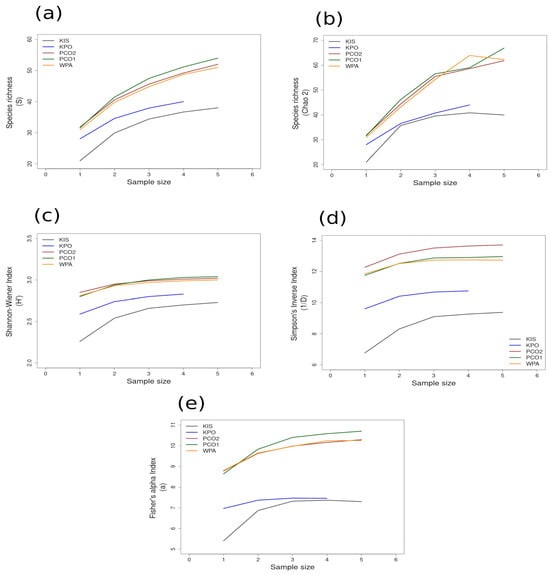
Figure 6.
Area curves plotted from incidence scoring for richness and diversity at sites within the cold temperate NAPF ecoregion in Southeast Alaska. Site abbreviations are the same as in Table 1. The diversity measures used for the curves are as follows: (a) species richness; (b) Chao 2 species richness estimator; (c) Shannon–Wiener; (d) Simpson’s Inverse; (e) Fisher’s alpha. Diversity and richness indices (y-axis) were calculated from randomized re-sampling of the sample-based incidence data from the transects (x-axis). Each curve shows the maximum estimated value, as computed by EstimateS v.9.1.0., for each site referenced in the text; standard deviations (SDs) were calculated but not added to the graph in order to preserve the clarity of the curve. Standard deviations for each diversity measure are provided in in the Supplementary Material Tables S6 and S7.
The lack of a pattern of richness among sites within ecoregions (α1) is consistent with the analysis of regional scale studies in marine systems, i.e., strong gradients of diversity in marine systems are atypical on local scales [61]. Site N5n1 in the HNS and site ENU in the GUAY ecoregions possessed the lowest incidences of rare species overall; the lowest computed species richness (S and Chao 2) and Fisher’s alpha biodiversity indices were found for ENU in the GUAY ecoregion. Bimodal peaks in richness were evident on medium (α2) spatial scales; for example, the estimations of the observed species richness were greater in the higher latitude ecoregions (Figure 7c and Figure 6d), while the Chao 2 richness estimator was greatest in the NAPF ecoregion. In the warm temperate and tropical ecoregions, both richness estimators were higher for the pooled GUAY sites (Figure 7a) compared to the HWS ecoregion (Figure 7b), and the Chao 2 richness estimator was highest for the HNS ecoregion (Figure 7c).
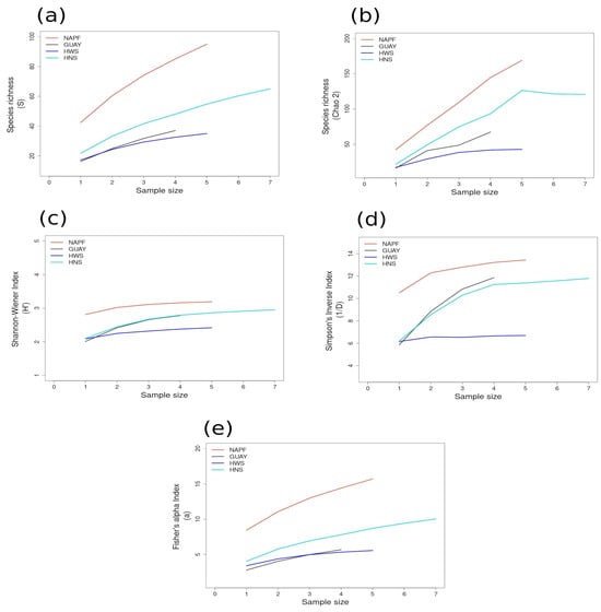
Figure 7.
Area curves plotted by diversity measure for comparison among all ecoregions: (a) species richness; (b) Chao 2 species richness estimator; (c) Shannon–Wiener Index; (d) Simpson’s Inverse Index; (e) Fisher’s alpha Index. Abbreviations for ecoregions are the same as in Table 1. Ecoregions are represented by color, as shown in the legends. Standard deviations for each diversity measure are provided in in the Supplementary Material Tables S6 and S7.
The large-scale estimated species richness was highest for the higher latitude ecoregions, implying a bimodal pattern of species richness in the higher temperate latitude ecoregions. The species richness area curves plotted for all the sites pooled by ecoregion are shown in Figure 8.
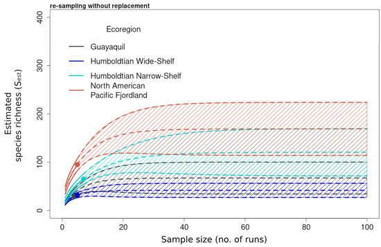
Figure 8.
Species accumulation curves of the estimated species richness (Sest) (solid lines) calculated from the reference samples from the incidence-based data pooled by ecoregion and extrapolated out to a sample size of 100 (dashed lines) with 95% upper and lower confidence intervals. Dots represent the end value of the reference sample and the beginning of the extrapolation. Richness values and confidence intervals were computed analytically through random re-sampling without replacement.
The large-scale (α3) accumulation curves for the functional/taxonomic group richness for NAPF showed the highest indices (Figure 9d) but also the greatest overestimation and underestimation of functional group richness, as suggested by the ±95% confidence intervals. The second highest curve was plotted for the GUAY ecoregion (Figure 9a), which also had a wide range of confidence intervals. Accumulation curves for both the HWS and HNS ecoregions were nearly identical to each other, with both showing comparatively narrower confidence intervals (Figure 9b,c).
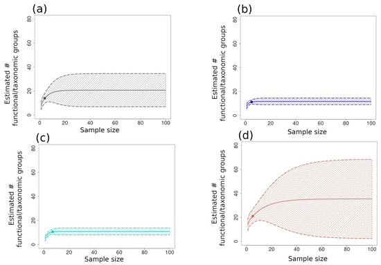
Figure 9.
Extrapolated functional/taxonomic group richness indices with 95% upper and lower confidence intervals plotted for pooled sites respective of each ecoregion, as follows: (a) GUAY (grey); (b) HWS (dark blue); (c) HNS (turquoise); (d) NAPF (brown). Th richness datum for each ecoregion was re-sampled without replacement. The dots on each graph show the x- and y-axes values for each of the samples, and shaded areas of the graph beyond the points are extrapolated values. The broad range of confidence intervals for the NAPF ecoregion indicate over- and underestimation of the extrapolated values.
The plots of the Hill numbers for each ecoregion revealed that the steepest decreasing curve was found between 0Δ (S) and 1Δ (Shannon Exponential Index) for all ecoregions. The curves show that relative abundances were more evenly distributed between the Shannon–Wiener and Simpson’s Inverse for all ecoregions. The highest overall q with the steepest negative curve was plotted for the NAPF ecoregion, with another steep curve plotted for the HNS ecoregion, implying a bimodal pattern of diversity and that the abundance of rare species (S) was uneven in distribution compared to the measures of typical and dominant species abundance [35]. The same characterization can be made for the Hill numbers plotted for the HNS ecoregions and, to a lesser extent, the HWS ecoregion, with the GUAY ecoregion showing the least variance in the distribution of richness and abundance of species (Figure 10).
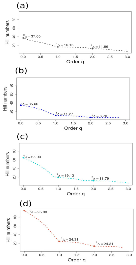
Figure 10.
Plots of the Hill numbers (q) from the sample-based incidence data (as indicated by Δ) from sites sampled in the (a) Guayaquil (gray plot); (b) Humboldtian Wide-Shelf (dark blue plot); (c) Humboldtian Narrow-Shelf (turquoise plot); and (d) North American Pacific Fjordland (brown plot). Hill numbers (q) are ordered from 0 to 2 and were computed from a binomial product model in EstimateS v.9.1.0. software for estimated species richness (0Δ); Shannon Wiener exponential form (1Δ); and Simpson’s Inverse (2Δ), as described in Chao et al. [35]. All graphs were plotted to the same scale in order to provide a perspective comparison of the steepness of each curve, where a steeper curve is an indicator of higher variation in abundance between measures.
3.2.2. Hutcheson’s t-Test of the Shannon–Wiener Indices
The results from the Hutcheson’s two-tailed t-tests for pairwise comparisons of the Shannon–Wiener indices are shown in Table 3. All but the pairwise comparison of Shannon–Wiener indices for sites ENU/CBL were significantly different (Bonferroni p < 0.008) in the GUAY ecoregion (Table 3); these two sites showed shared characteristics of high levels of disturbance; for example, site CBL was impacted by a mudslide during sampling and site ENU receives periodic sand loading in the intertidal zone. Six pairwise comparisons within the HWS ecoregion (PFA1/PEN, PFA2/PEN, PGA/PEN, PFA1/PFA2, PFA1/PGA, and PFA2/PGA) (Table 3), two comparisons in the HNS ecoregion (S5/P7H2b and P7H2a/P7H2b) (Table 3) and in the NAPF ecoregion (PCO1/PCO2, PCO1/WPA, and PCO2/WPA) (Table 3) were not significantly different in their Shannon–Wiener diversity indices. Proximal distances were shortest between the sites at P7H2a and -b, PFA1 and -2, and PCO1 and -2 (please see Table S1 in the Supplementary Material).
Table 3.
Results for the α2 scale Hutcheson’s t-test for significance of differences in the Shannon–Wiener diversity indices, with an alpha < 0.008 among sites within ecoregions. Please see Table 1 for ecoregion and site abbreviations and corresponding names. Variances shown next to Bonferroni p-values.
On the largest (α3) scale, significant differences in Shannon–Wiener indices were found among all ecoregional pairs (p < 0.008), with the greatest variation (32.38) between the HNS and GUAY ecoregions (Table 4).
Table 4.
Results for the α3 scale Hutcheson’s t-test for significance of difference in Shannon–Wiener diversity indices among ecoregions (sites were pooled sites respective to each ecoregion). Variances shown next to significant Bonferroni p-values.
3.3. Beta Diversity
3.3.1. Patterns of Zonation: β1 Scale
The intertidal zones of the GUAY, HWS, and HNS ecoregions were broadly characterized by algae of lower functional complexity (foliose and filamentous) and barnacles and periwinkles (Family Littorinidae) in the high to middle intertidal zones, while species of algae belonging to a higher order of functional groups (e.g., leathery macrophytes) and the acorn barnacle Balanus glandula Darwin, 1854, dominated the upper zones of the NAPF ecoregion. Green foliose algae (fx. group 3) from the genus Ulva and the crustose red alga Lithothamnion (fx. group 7) were present in the lower zones at most sites throughout all of the ecoregions. The census of the articulated calcareous alga C. chilensis, a species that was recently considered to be a variation of C. officinalis but for which phylogenetic analysis has established it to be a separate species [57,59], was remarkable for being found at a single location in the warm temperate HNS ecoregion. The range for C. chilensis has been described from Alaska to Chile; however, its range in Peru has yet to be substantiated [58,59,60]. The verification of C. chilensis in the HNS ecoregion of Peru in this study underscores the importance of conducting a census on understudied regions and providing an inventory of species to be used for future studies; Corallina have been used as proximal species for assessing the magnitude of ocean acidification and the cascading effects on other calcifying marine biota in warm and cold temperate marine biomes [62,63,64,65].
The Bray–Curtis similarity analysis provided a coherent picture of species turnover in the intertidal zones along delineated gradients at each site. All of the β1 scale nMDS ordinations and clusters with single linkage dendrograms for each of the sites can be found in the Supplementary Materials Figures S1–S26 and Tables S8–S38 and are not referenced in numeric order from this point forward. Because of the irregularity of the substrates at sites N5n2, S5, S4, P7H2a, and P7H2b (HNS) where it was not possible to score along a continuous transect, 70 cm × 50 cm quadrats were used for scoring in order to compute the groupings for ordinating the nMDS and cluster dendrograms (Figures S11, S13–S16). All sites within the NAPF ecoregion were ordinated into groups of high and medium zones (Figures S18–S22), and in the warm temperate and tropical ecoregions, sites ACA (GUAY) (Figure S1), PEN (HWS) (Figure S6), and UOA (HNS) (Figure S17) were ordinated into groups of low, high, and mid zones. The ordination for PEN showed location/dispersion effect differences among the groups. All of the ordinations showed the strongest ordinal correlations for axis 1, with the exception of PVE (r2 = 0.22, Figure S4), with the highest axis 1 value computed for PGA (r2 = 0.90) (Figure S9). The post hoc PERMANOVA values were significant for all sites with the exception of N5n2, S4, S5, P7H2a, and P7H2b, which were excluded from the test due to the indistinct nature of the clustering during the nMDS ordinations. F statistic values from the test were discrete between 2 and 9. Distances among the clusters for all dendrograms, except for S5 (r2 = 0.08), were strongly preserved with a minimum cophenetic r2 value of 0.76 computed for CBL (Figure S2). In some instances, there was a combination of zones clustered at similarity >0.50, which could be the result of perturbations affecting the communities within that section of the zone, such as elevation of the substrate, tide pools, and freshwater influence, that may harbor communities that are more or less similar to other zones. For example, one cluster combined a sample from the mid zone at KIS clustered with samples from the high zone (Figure S18). KIS was characterized by numerous tidepools and fluctuations in elevation along the transects resulting in areas that were awash by the incoming tide well before the lower areas on the transect were awash, and this was also the case for other sites that showed similar effects among zones. Aside from this, the zones were significantly different overall. The envfit multiple regression analysis revealed that there were significant and strong associations between many of the environmental variables (algae and invertebrates) and the ordination axes that characterized the dissimilarities among the zones (Tables S8–S29). The greatest number of species from the multiple regression for the zones in the warm temperate and tropical ecoregions was found for UOA, with six algae and five invertebrates accounting for differences among the zones (r2 ≥ 0.40), and six algae and six invertebrates at WPA (NAPF) in the cold temperate ecoregion (Table S29).
In the GUAY ecoregion, the brown alga Padina durvillei (Bory), the red alga Hypnea valentiae (Montagne), and the hermit crab Pachygrapsus transversus (Gibbs, 1850) characterized the low zone. The mussel Brachidontes characterized the mid zones of ACA, CBL, and ENU (Tables S8–S10), the periwinkle Echinolittorina paytensis (R.A. Philippi, 1847) and the barnacles Jehlius cirratus (Darwin, 1854) characterized the mid zones of CBL and ENU, and Notochthamalus scabrosus (Darwin, 1854) was also significant in the mid zones of CBL and ENU. In the high zone, ENU was characterized by the green filamentous alga Chaetomorpha cartilaginea Howe, the red corticated alga Chondracanthus glomeratus (Howe) and the red crust Hildenbrandia sp., E. paytensis, and the limpet Siphonaria lessoni Blainville, 1827. The filamentous green algae Acrosiphonia (Agardh) sp. was significant at CBL, and an unidentified colonial anemone was significant at ACA.
In the HWS ecoregion, where the delineations in the zones were between mid and high, Echinolittorina peruviana (Lamarck, 1822) was significant in the high zone and the anemones Oulactis concinnata (Drayton in Dana, 1846) and Phymactis papillosa (Lesson, 1830) were significant in the mid zone. The corticated red alga Ahnfeltia durvillei var. implicata (Kützing) and the red articulated calcareous alga C. officinalis were significant in the mid zones at PFA1 (Table S14) and PFA2 (Table S15), while an unknown filamentous green alga and the brown leathery macrophyte Petalonia fascia (O.F. Müller) were also significant in the community structure at PFA1, and the mussels P. purpuratus and S. algosus along with the limpet Scurria viridula (Lamarck, 1819) were significant in the community structure at PFA2. P. purpuratus was also significant in the mid zone at LDO along with the green foliose alga Ulva rigida C. Agardh, (Table S12), also significant in the mid zone at PGA (Table S16). In the high zone, E. peruviana was significant at PEN (Table S13) and LDO, P. fascia was significant at PFA1, and N. scabrosus was significant at LDO and PGA. The brown crust alga Ralfsia sp. was only found at PGA and was significant to the structure of the high zone. At N5n1 in the HNS ecoregion, a brown micro-alga was significant for delineating the high zone, blue-green algae found on the plates of barnacles and shells of mussels, the barnacle N. scabrosus, and the limpet S. viridula were all characteristic of the mid zone (Table S17). Because the methods used to define zonation along a transect were not used at plots N5n2, S5, and S4, P7H2a, and P7H2b, all species significant in the ordinations were assigned as belonging to quadrant I through quadrant IV in the ordinations of the nMDS plots (Tables S18 and S20–S23). At UOA, the low zone was characterized by an unidentified brown macrophyte alga, Ceramium sp., Colpomenia sinuosa (Mertens ex Roth), H. helianthus, Lithothamnium sp., Phymactis clematis (Drayton in Dana, 1846), U. rigida, and the invasive solitary tunicate P. praeputialis. The hornsnail Incatella cingulata (G.B. Sowerby I 1825) as well as E. peruviana was strongly correlated with the high zone, and a Chaetomorpha sp. characterized the mid zone (Table S24).
In the NAPF ecoregion, the high zone was significantly characterized by the acorn barnacle Balanus glandula Darwin, 1854, at KIS (Table S25), KPO (Table S26), and WPA (Table S29), also significant at PCO1 (Table S27) in the mid zone. The leathery macrophyte Fucus gardneri P.C. Silva, was significant in the high zone at KIS, and PCO1, and in the mid zone at KPO. MYTCOM was significant in the mid zone at KPO, the high zone at WPA, and the high and mid zone at PCO2 (Table S21). The red filamentous algae Pterosiphonia bipinnata (Postels & Ruprecht) was significant in the mid zone at KIS, KPO, PCO2, and in the mid zone at WPA (Table S29). As well as the above, KIS was characterized by anemones (Anthopleura xanthogrammica, Brandt, 1835), blue green algae, crustose and leathery macrophyte algae (Hildenbrandia sp. and F. gardneri respectively) in the high zone, and mussels, the giant acorn barnacle Semibalanus cariosus (Pallus, 1788), and brown and red algae, namely Odonthalia floccosa (Esper) and P. bipinnata respectively. Other than F. gardneri, KPO was also characterized by green and red algae (Codium setchelli N.L. Gardner, Ulva lactuca Linnaeus, and P. bipinnata, and Mastocarpus sp., respectively) along with the limpet Lottia paradigitalis (Fritchman, 1960) in the mid zone. At PCO1, the periwinkle Littorina scutulata Gould, 1849, and S. cariosus also characterized the high zone, the green foliose alga Ulvaria was significant in the high and mid zone, and the thatched barnacle Chthamalus dalli Pilsbry, 1916, the limpet Lottia asmi (Middendorff, 1848), Ulvaria sp., and the corticated red algae C. vancouveriensis were significant in the mid zone. At PCO2 Ulvaria sp. was significant in the high and mid zone and U. lactuca, the periwinkle Littorina sitkana R.A. Philippi, 1846, and a barnacle (suggested as an Amphibalanus sp.) were also significant in the high zone, while A. xanthogrammica, P. bipinnata, and the leathery kelp Alaria nana H.F. Schrader, were significant in the mid zone. At WPA, blue-green alga, L. scutululata, S. cariosus, and Amphibalanus, were significant in the high zone, and in the mid zone the introduced brown alga Analipus japonicus (Harvey), C. setchelli, red algae, such as Hildenbrandia sp., Mastocarpus jardinii (J. Agardh), Lithothamnion, as well as A. xanthogrammica, were significant.
3.3.2. Patterns of Similarity: β2 Scale
The β2 scale ordinations all suggested stronger r2 values along axis 1, with the strongest value for the NAPF ordination (r2 = 0.72, Figure S26). The post hoc PERMANOVA values were all significant (p < 0.001, Table S36). The nMDS ordination for the GUAY ecoregion showed a dispersion/location effect among most groups, however the dendrograms revealed that sites and zones within sites were generally clustered together at ~0.50–0.60 similarity (Figure S23). The GUAY sites were among the lowest in richness and diversity, and the level of disturbance (erosion and sand loading) could be responsible for hierarchical succession of lower complexity algae and invertebrates. For example, the foliose green algae U. rigida and an unidentified but abundant colonial anemone were significant for differences with strong r2 correlations (0.51 and 0.48 respectively, Tables S30 and S31). The β2 scale nMDS ordinations of the GUAY ecoregion suggests location effects among the sites.
In the ordination for the HWS ecoregion, the clusters for sites LDO and PGA displayed location effect while the remaining groups displayed location/dispersion effects across the axes. Groups were generally clustered at ~0.70–0.80 similarity in the dendrogram, with a few samples illustrating low similarity values within their cohorts. This was most obvious for PEN (HWS), which had one large and several small tidepools bisected by the transects (Figure S24). The post hoc PERMANOVA revealed no significant differences (Bonferroni p = 0.005) between PEN and PFA1 (p = 0.37) and PFA2 (p = 0.24) and PFA1 and PFA 2 (p = 0.33, Table S32). LDO possessed the lowest species richness and also experiences a high level of disturbance, as there was heavy foot traffic in the intertidal zone witnessed at the time of sampling. In the ordination for the HNS ecoregion, the clusters for UOA and N5n1 displayed location/dispersion effect, all other sites were dispersed across the axes (Figure S25). Similar to LDO (HWS), sites N5n1 and N5s possessed the lowest species richness as well as a high level of observed disturbance from South American Sea lions hauling out of the water. Sites S4 and S5, P7H2a and b, N5n2 and S4, and P7H2b and UOA were not significantly different, respectively (Table S34). In the ordinations for the NAPF ecoregion, KIS, PCO2, and PCO1 displayed location effects, while WPA and KPO displayed location/dispersion effects (Figure S26). Significant p-values were calculated for the variations between sites PCO1 and 2, with the greatest distance between clusters, while KPO and PCO1, KIS and PCO1, KIS and KPO were not significant in variation (Table S36).
A colonial anemone was a significant characteristic of ACA, while U. rigida was a significant characteristic of ENU, setting the two sites apart from other sites in the GUAY ecoregion (Table S31). The red algae Chondracanthus chammissoi (C. Agardh) and C. glomeratus were significant for characterizing PGA apart from the rest of the sites in the HWS ecoregion (Table S33), E. peruviana was significant for characterizing N5n2 and N5S apart from the rest of the sites in the HNS ecoregion (Table S35), and A. nana and A. xanthogrammica were significant for characterizing PCO2 and KIS apart from the rest of the sites in the NAPF ecoregion (Table S37).
3.3.3. Patterns of Similarity: β3 Scale
The β3 scale Sorensen–Dice ordinations of the taxonomic and functional groups across all ecoregions displayed location effect for the NAPF and HWS ecoregions, and the GUAY and HNS groupings were location/dispersed (Figure 11a), while the corresponding dendrogram displayed short axial and linkage distances among the ecoregional clusters (Figure 11b). Functional diversity can be affected by disturbance in the community [29]. The Sorensen–Dice cluster analysis suggested that WPA (NAPF) was highest in terms of functional similarity (Sorensen–Dice similarity~0.65) to the warm temperate and tropical sites when compared to other sites within the NAPF ecoregion. The remaining sites in the NAPF ecoregion shared similarity ~0.80, with PCO1 sharing similarity with sites KIS and KPO when compared to PCO2. The cluster analysis suggested that CBL (GUAY) was least similar to any of the ecoregions, likely as a result of significant disturbance event at the time of sampling (floods that brought sediment from a nearby mountainside to the intertidal zone during the coastal El Niño of 2017), and the intertidal zone at PVE (GUAY) is impacted seasonally by temporal sand loading. Sites PFA1 and PFA2 (HWS), and P7H2a (HNS) and PEN (HWS) shared the highest similarity index~0.95.

Figure 11.
Multivariate graphical descriptions of the β3 scale Sorensen–Dice (a) nMDS ordination with stress < 0.20, PERMANOVA p-value < 0.001 and r2 values given for the correlation between each axis and the cluster ordination and (b) cluster dendrogram with the cophenetic correlation values > 0.50. Clusters represent the taxonomic and functional groups of the sampled intertidal communities for all ecoregions. Colored dots in the ordination graphs and text in the dendrograms represent the ecoregion each site belongs to gray = GUAY (Guayaquil) ecoregion, dark blue = HWS (Humboldtian Wide-Shelf) ecoregion, turquoise = HNS (Humboldtian Narrow-Shelf) ecoregion, and brown = NAPF (North American Pacific Fjordland) ecoregion. Abbreviations in (b) indicate sites.
The post hoc analysis revealed that the structures of the taxonomic and functional groups were significantly similar among all ecoregions (Bonferroni p < 0.008, Table 5), with spatial overlap between sites in the HNS and HWS ecoregions at a Sorensen–Dice similarity ≥0.70. Most sites from the NAPF ecoregion were clustered together with linkage at ≥0.80 except for WPA, which along with CBL (GUAY) shared linkage with a similarity index ≤0.65.
Table 5.
Results from the post hoc PERMANOVA for testing the variance of taxonomic and functional groups among all ecoregions in the nMDS ordination. Significance at Bonferroni p < 0.008.
The NAPF ecoregion accounted for most of the significant (Pr{>r}, r2 > 0.40) variables (taxonomic and functional groups) in the nMDS ordinations, with red filamentous algae (fx. Group 2.5), corticated foliose algae (fx. Group 3.5), leathery macroalgae (fx. Group 5), theostracans (barnacles), eumalocostracans (hermit crabs), patellogastropods (limpets), and zoantherids characteristic of the functional structure of the region, while the heterobranch limpet Siphonaria lessoni characterized the GUAY ecoregion (Table 6).
Table 6.
A list of the functional and taxonomic groups along with r2 values > 0.40 and significant sequential p-values (<0.05) from the post hoc multiple regression analysis (envfit) of Jaccard distances for all ecoregions (GUAY, HWS, HNS, and NAPF).
4. Discussion
Latitudinal gradients of species richness in benthic and pelagic marine ecosystems do not necessarily follow the monotonic pattern of terrestrial systems and are less apparent on local scales, with one peak near the equator and another smaller peak at higher latitudes [61,66,67]. The latitudinal gradient in species richness theory has been tested primarily on marine benthic and pelagic habitats where temperature, habitat, species morphology and other variables are correlated with species richness [61,67]. The revitalized effort to compare intertidal communities in terms of species richness and diversity on local scales has produced various results based on the diversity methods used, the scale of the study, and abiotic factors [6,68,69]. The peaks in species richness identified at 5° S and 12° S by Valqui et al. [1] were found to be associated with the magnitude of herbivory [29] in addition to dissolved oxygen, nutrients, and seawater temperatures, and the results for richness and diversity prevalent in our study support this the same pattern where species richness was found to be higher in the cold and warm temperate ecoregions, where higher inorganic nutrient availability and phytoplankton productivity is a feature of the mid-latitude regions as proposed by Chaudhary et al. [66].
Steneck and Dethier [29] have proposed that the factors governing an ecosystem’s productivity potential, i.e., success in terms of propagation and rate of biomass for any number of functional algal groups, plus the properties of the environment that facilitate these successes, and disturbance potential (the frequency of events that result in the loss of biomass) are linked to total algal biomass and functional algal diversity. Konar et al.’s [5] exploration of depth-stratified taxonomic richness in central Alaska intertidal/subtidal communities revealed coherent patterns richness on the broadest scale within the scope of their research, and our trans-ecoregional approach to finding a coherent pattern of functional and taxonomic group similarity among intertidal communities is unique and deserves further attention as similar research effort is undertaken. We place emphasis in our discussion on the geographic features of the rocky intertidal substrates and disturbance potential as they relate to the structure and richness of the biological communities. There was evidence of seasonal sand loading were factors could be the cause of disturbance at the sites in the intertidal zones of the tropical GUAY ecoregion; for example, mudslides and severe flooding affected some of the intertidal areas during the Coastal El Niño where algal species belonging to groups of lower functionally complexity were mostly found. The sites at CBL and PVE (GUAY) with low species turnover and low diversity were characteristic of the rocky intertidal platforms of the northern Peruvian coast where disturbance affects the hierarchical structure of the communities [1], where both sites were subject to high seasonal sand loading with scattered colonies of small barnacles and no mussels assemblages lower in the tide zone. Switzer [70] has described several theories that explain why certain species exhibit site or habitat fidelity as well as the inverse relationship between optimal and suboptimal habitats. Inverse relationships include the ability to mitigate abiotic stressors such as temperature and desiccation in return for increased risk of depredation and foraging and reproductive success. We suggest that the species at these sites that inhabit the high and mid zones establish quickly following a disturbance, or in the case of motile invertebrates, shelter in niche habitats where disturbance is mitigated. Other sites that were periodically submerged by the coastal sediments transported southward by coastal counter currents. To date, the duration of sand loading and re-emergence of the substrate at the affected sites has not been measured, however the apparent dominance of a fast growing and morphologically diverse species from the genus Ulva, which can tolerate extreme environments that prevent higher complexity species of algae to establish, provides biological evidence of disturbance [71].
The intertidal zones of the HWS and HNS ecoregions did not outwardly appear to be affected by disturbance from sand loading; however, chronic disturbance in some areas was evident in the form of human foot traffic and the fishing of invertebrates and algae for personal and commercial use. The angled slabs of rock benches and rock vertices of the HWS and HNS ecoregions were characteristic of a tectonically active landscape [72] with numerous boulders littering the intertidal zone. The addition of rocky substrates as material is released from the surrounding cliff faces during a tremor suggests that earthquakes are an acute form of disturbance in the landscape. Subduction and uplift have been shown to reduce or increase habitat availability in the intertidal zone with consequent impacts to associated communities [73], as was evidenced by the boulders dislodged from nearby cliff faces littering the intertidal zones in the HWS and HNS ecoregions. Where the area of substrate was limited, the communities were characterized by high species turnover and relatively low alpha diversity, with the lowest boundary of the intertidal zone dominated by actinids. Disturbance from wave forces and upwelling play a role in diversity through larval recruitment in the foundation species of intertidal communities [74,75,76]. Sites at Reserva San Juan possessed relatively higher diversity compared to other sites within the HNS ecoregion, likely due to the close proximity of the Reserve to upwelling from the Humboldt Current System [77]; the presence of nesting colonies of sea birds as well as South American sea lions and fur seals that also colonize near the shoreline are evidence of the area’s high productivity. The variations in alpha diversity in the intertidal communities there may be due to higher levels of disturbance versus higher levels of productivity, influenced by factors involving upwelling and wave force [16]. Sites in the NAPF ecoregion possessed rocky substrate that extended well into the subtidal areas, characteristic of a transitional geography driven by isostatic rebound of historically glaciated bedrock [78,79,80]. In high-latitude glaciated fjord regions, rock faces near the termini of retreating tidewater glaciers are the ultimate example of postdisturbance substrate for intertidal succession species, and this is evidenced in bands of Ulva colonizing exposed rocks near the Dawes Glacier (NAPF) (Figure 12).
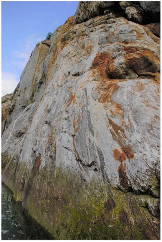
Figure 12.
Foliose green algae from the genus Ulva colonizing the intertidal zone near Dawes Glacier in Southeast Alaska, an area of recent postglacial retreat, where light is limited at high tide due to suspended colloidal material in the water. The photo demonstrates the ability of this species to colonize in areas of high disturbance.
Climate change is playing an ever more prevalent role in disturbance in high latitude intertidal ecosystems, as the accelerating rate of glacial retreat in the northeastern Pacific has also increased the vertical area of available intertidal substrate for the colonization of intertidal communities [81], resulting in an increase in the exposure times of successive intertidal biota to atmospheric extremes at low tide. Questions surrounding the dynamics of the delivery of inorganic nutrients to marine systems from glacial runoff have yet to be answered, but the relationship between iodine uptake and efflux in kelps and the formation of coastal fog is well known [82], yet the acceleration of climate change has introduced a new challenge to researchers in terms of disturbance to intertidal systems with fewer days of coastal fog and cloud cover during the boreal summer months corresponding with mass mortality occurring in invertebrate populations and mass algal bleaching (the loss of chlorophyll pigments as a result of cell die-off, Figure 13).

Figure 13.
The red turf seaweed Endocladia muricata (Endlicher), a species that forms dense covers in the mid intertidal zone of the NAPF ecoregion, is shown here denuded of cellular pigments at KIS in the summer of 2018 following an extended period of higher-than-average air temperatures. The first case of algae bleaching was documented at KPO in canopy kelps in the summer of 2016.
Some of the patterns of similarity shown in the functional group dendrograms suggest higher levels of similarity across all ecoregions in congruence with Steneck and Dethier’s General Model of the inverse relationship between disturbance potential and functional group complexity [28]. In other words, disturbance potential from geological forcing may be lower in communities with relatively high functional group complexity, and there may be an underlying indication of the resilience of these communities following acute disturbance. As marine heatwaves become an increasingly frequent event in the Gulf of Alaska [83,84,85,86] and forcings at the air-sea interface intensify as a result of climate change creating stronger and more frequent El Niños impacting the Eastern Pacific, the predictions for marine systems include dramatic shifts in the species ranges, trophic structure, and functional group hierarchies of the biological communities [9,87,88,89]. All of these factors pose major implications for diversity and richness in the intertidal communities as well.
5. Conclusions
This multiscale spatial analysis of rocky intertidal ecosystems in Eastern Pacific cold temperate, warm temperate, and tropical ecoregions has provided valuable data on patterns of diversity and zonation across a broad and diverse geographic scale. Our analysis of hundreds of algal and invertebrate species across cold temperate, warm temperate, and tropical Eastern Pacific ecoregions confirmed that unlike terrestrial systems, a biomodal pattern of richness exists in marine systems. Such a broad-scale census of intertidal communities can assist us in developing a better understanding of patterns of alpha and beta diversities and how they vary across the northeast and southeast Pacific, and perhaps provide us with the tools necessary for predicting resilience and change in these communities as a result of climate change.
Supplementary Materials
The following supporting information can be downloaded at: https://www.mdpi.com/article/10.3390/d16080498/s1, Figures S1–S26: nMDS ordinations and dendrograms of β1 and β2 scale community clusters by site and ecoregion. Figure S27 (a) and (b): Bar charts showing percentages of mobile species that utilize niche space based on the abundance surveys. Figure S28 (a–d): Three marine gastropods from the family Rapininae and one marine gastropod from the family Littorinidae sampled from the GUAY and HWS ecoregions. Table S1: Matrix of distances among sites. Table S2: List of species, NAPF ecoregion. Table S3: List of species, GUAY, HWS, HNS ecoregions. Table S4: Rocky intertidal zone characterizations. Table S5: Total area data sampled. Table S6: Mean diversity index values computed by EstimateS v.9.1.0. software. Table S7: Mean species richness index values computed by EstimateS v.9.1.0. software. Tables S8–S29: Tables of significant species, r-squared and p-values from the post hoc multiple regression analysis from the β1 nMDS ordinations. Tables S30, S32, S34, S36: p-values from the post hoc PERMANOVA test for differences among sites within ecoregions. Tables S31, S33, S35, S37: Table of significant species with r2 ≥ 0.40 and p-value calculated by permutation test from the post hoc envfit multiple regression of the nMDS for each ecoregion. Table S38: Index values of species richness (S) and Shannon Wiener (UH’) diversity from the rarefied abundance survey data of individuals of mobile species counted in the niche habitats. Table S39: A list of mobile species identified to highest taxonomic classification that were encountered during the abundance surveys according to sites in the GUAY, HWS, and HNS ecoregions. Table S40: A list of the mobile species identified to highest taxonomic classification that were encountered during the abundance surveys according to sites in the NAPF ecoregion. References [90,91,92,93,94,95,96,97,98,99] are cited in the supplementary materials.
Author Contributions
Conceptualization, L.W.; methodology, L.W.; formal analysis, L.W. and V.L.; investigation, L.W. and F.C.K.; Resources, L.W. and F.C.K.; data curation, L.W. and F.C.K.; writing-original draft preparation, L.W. and V.L.; writing—review and editing, L.W. and V.L.; supervision, F.C.K. and V.L.; funding acquisition, L.W. and F.C.K. All authors have read and agreed to the published version of the manuscript.
Funding
This research was funded by the Marine Alliance for Science and Technology for Scotland. MASTS is funded by the Scottish Funding Council (funding number HR09011).
Data Availability Statement
The data presented in this manuscript and in the Supplementary Materials is available upon request from the authors.
Acknowledgments
The authors would like to express their appreciation and thanks to Marco Cardeña Mormontoy andthe Rangers and staff at the Reserva Punta San Juan in San Juan de Marcona, Peru, and to Yuri Hooker-Mantilla and Susana Cárdenas Alayaza from the Center for Environmental Sustainability at Universidad Peruana de Cayetano Heredia (UPCH) in Lima, Peru, for their partnership, supervision, assistance with permitting, and fieldwork; to Bruno Ibanez Erquiaga for his assistance with fieldwork and logistics; to Henry Larsen for his assistance in the field; to Eduardo Salcedo for his unconditional support as a liaison with UPCH administrative staff; to Ros.marie Hardmeier at UPCH for making the Memorandum Agreement between UPCH and University of Aberdeen a reality; to the Ministero de la Producción de Peru (PRODUCE) for providing the permit to collect marine specimen; the Servicio Nacional de Áreas Naturales (SERNANP) for their permission to conduct field work within the Reserve; to Shaleyla Kalez of EcoOceanica for her assistance with lodging and other logisitics in the Guayaquil ecoregion of Peru; to Professor Aldo Pacheco at the Universidad de Antofagasta for opening his home and helping with logistics and species identification in the Chilean portion of the Humboldtian Narrow-Shelf ecoregion. Our heartfelt thanks goes to Marina Sissini at PELD ILOC for sequencing the marker from our articulated calcareous algal specimen to the Hidalgo family (Carlos Justo Hidalgo, Mercedes Venegas Guzman, Carlos Hidalgo, and Monica Hidalgo) for opening their home in Lima and offering their undying friendship and support during our field seasons; to Carolina Linan Rojas for her friendship and help with forming the necessary partnerships. This study was partially supported by the University of Aberdeen School of Biological Sciences.
Conflicts of Interest
The authors have no conflicts of interest to declare.
References
- Ibanez-Erquiaga, B.; Pacheco, A.S.; Rivadeneira, M.M.; Tejada, C.L. Biogeographical Zonation of Rocky Intertidal Communities along the Coast of Peru (3.5–13.5° S Southeast Pacific). PLoS ONE 2018, 13, e0208244. [Google Scholar] [CrossRef]
- Valqui, J.; Ibañez-Erquiaga, B.; Pacheco, A.S.; Wilbur, L.; Ochoa, D.; Cardich, J.; Pérez-Huaranga, M.; Salas-Gismondi, R.; Pérez, A.; Indacochea, A.; et al. Changes in Rocky Intertidal Communities after the 2015 and 2017 El Niño Events along the Peruvian Coast. Estuar. Coast. Shelf Sci. 2021, 250, 107142. [Google Scholar] [CrossRef]
- Bosman, A.L.; Hockey, P.A.R.; Siegfried, W.R. The Influence of Coastal Upwelling on the Functional Structure of Rocky Intertidal Communities. Oecologia 1987, 72, 226–232. [Google Scholar] [CrossRef]
- Bustamente, R.H.; Branch, G.M.; Eekhout, S.; Robertson, B.; Zoutendyk, P.; Schleyer, M.; Dye, A.; Hanekom, N.; Jurd, M.; McQuaid, C.; et al. Gradients of Intertidal Primary Productivitiy around the Coast of South Africa and Their Relationships with Consumer Biomass. Oecologia 1994, 102, 189–201. [Google Scholar] [CrossRef]
- Konar, B.; Iken, K.; Edwards, M. Depth-Stratified Community Zonation Patterns on Gulf of Alaska Rocky Shores. Mar. Ecol. 2008, 30, 63–73. [Google Scholar] [CrossRef]
- Okuda, T.; Noda, T.; Yamamoto, T.; Ito, N.; Nakaoka, M. Latitudinal Gradient of Species Diversity: Multi-Scale Variability in Rocky Intertidal Sessile Assemblages along the Northwestern Pacific Coast. Popul. Ecol. 2004, 46, 159–170. [Google Scholar] [CrossRef]
- Menge, B.A. Predation Intensity in a Rocky Intertidal Community: Relation between Predator Foraging Activity and Environmental Harshness. Oecologia 1978, 34, 1–16. [Google Scholar] [CrossRef] [PubMed]
- Menge, B. Top-down and Bottom-up Community Regulation in Marine Rocky Intertidal Habitats. J. Exp. Mar. Biol. Ecol. 2000, 250, 257–289. [Google Scholar] [CrossRef] [PubMed]
- Steneck, R.S.; Watling, L. Feeding Capabilities and Limitation of Herbivorous Molluscs: A Functional Group Approach. Mar. Biol. 1982, 68, 299–319. [Google Scholar] [CrossRef]
- Engle, J.M. Unified Monitoring Protocols for the Multi-Agency Rocky Intertidal Network; U.S. Department of the Interior Minerals Management Service Pacific OCS Region: Camarillo, CA, USA, 2008; Volume 1, p. 84.
- Bell, E.C. Environmental and Morphological Influences on Thallus Temperature and Dessication of the Intertidal Alga Mastocarpus Papillatus. J. Exp. Mar. Biol. Ecol. 1995, 191, 29–55. [Google Scholar] [CrossRef]
- Harley, C.G.D.; Helmuth, B. Local and Regional Scale Effects of Wave Exposure, Thermal Stress, and Absolute versus Effective Shore Level on Patterns of Intertidal Zonation. Limnol. Oceanogr. 2003, 48, 1498–1508. [Google Scholar] [CrossRef]
- Helmuth, B.; Miezkowska, N.; Moore, P.; Hawkins, S.J. Living on the Edge of Two Changing Worlds: Forecasting the Responses of Rocky Intertidal Ecosystems to Climate Change. Annu. Rev. Ecol. Evol. Syst. 2006, 37, 373–404. [Google Scholar] [CrossRef]
- Helmuth, B.; Broitman, B.R.; Blanchette, C.A.; Gilman, S.; Halpin, P.; Harley, C.D.G.; O’Donnell, M.J.; Hofmann, G.E.; Menge, B.; Strickland, D. Mosaic Patterns of Thermal Stress in the Rocky Intertidal Zone: Implications for Climate Change. Ecol. Monogr. 2006, 76, 461–479. [Google Scholar] [CrossRef]
- DeVogelaere, A.P.; Foster, M.S. Damage and Recovery in Intertidal Fucus Gardneri Assemblages Following the “Exxon Valdez” Oil Spill. Mar. Ecol. Prog. Ser. 1994, 106, 263–271. [Google Scholar] [CrossRef]
- Wilbur, L.; Küpper, F.C.; Louca, V. Algal Cover as a Driver of Diversity in Communities Associated with Mussel Assemblages across Eastern Pacific Ecoregions. Mar. Ecol. 2023, 45, e12785. [Google Scholar] [CrossRef]
- Spalding, M.D.; Fox, H.E.; Allen, G.R.; Davidson, N.; Ferdaña, Z.A.; Finlayson, M.; Halpern, B.S.; Jorge, M.A.; Lombana, A.; Lourie, S.A.; et al. Marine Ecoregions of the World: A Bioregionalization of Coastal and Shelf Areas. BioScience 2007, 57, 573–583. [Google Scholar] [CrossRef]
- Wilbur, L.; Louca, V.; Ibanez-Erquiaga, B.; Küpper, F.C. A Case for Trans-Regional Intertidal Research in Unstudied Areas in the Northeast and Southeast Pacific: Filling the Gaps. Coasts 2024, 4, 323–346. [Google Scholar] [CrossRef]
- Arakaki, N.; Carbajal, P.; Gamarra, A.; Gil-Kodaka, P.; Ramírez, M. Macroalgas de la Costa Central del Perú; Universidad Nacional Agraria La Molina: Lima, Peru, 2019; p. 128. ISBN 978-612-4387-19-7. [Google Scholar]
- Dawson, Y.E.; Acleto, C.; Foldvik, N. The Seaweeds of Peru; Weinheim Verlag Von J. Cramer: Stuttgart, Germany, 1964; p. 111. ISBN 978-3-7682-5413-7. [Google Scholar]
- Howe, M.A. Marine Algae of Peru; Memoirs of the Torrey botanical club; Press of the New era Print. Co.: New York, NY USA, 1914; p. 285. [Google Scholar]
- Instituto del Mar del Perú. Catálogo Digital de La Biodiversidad Acuática Del Perú. Available online: https://biodiversidadacuatica.imarpe.gob.pe/ (accessed on 20 May 2024).
- Abbott, I.A.; Hollengerg, G.J. Marine Algae of California; Stanford University Press: Redwood City, CA, USA, 1976; p. 844. [Google Scholar]
- Carlton, J.T. Intertidal Invertebrates from Central California to Oregon the Light and Smith Manual, 4th ed.; University of California Press: Redwood City, CA, USA, 2007; p. 1001. [Google Scholar]
- Kozloff, E. Marine Invertebrates of the Pacific Northwest with Additions and Corrections; University of Washington Press: Seattle, WA, USA, 1996; p. 539. ISBN 978-0-295-97562-7. [Google Scholar]
- AlgaeBase:: Listing the World’s Algae. Available online: https://www.algaebase.org/ (accessed on 12 July 2024).
- Steneck, R.S. Herbivory on Coral Reefs: A Synthesis. In Proceedings of the 6th International Coral Reef Symposium, Townsville, Australia, 8–12 August 1988; Volume 1, pp. 37–49. [Google Scholar]
- Steneck, R.S.; Dethier, M.N. A Functional Group Approach to the Structure of Algal-Dominated Communities. Oikos 1994, 69, 476–498. [Google Scholar] [CrossRef]
- Steneck, R.S.; Vavrinec, J.; Leland, A.V. Accelerating Trophic-Level Dysfunction in Kelp Forest Ecosystems of the Western North Atlantic. Ecosystems 2004, 7, 323–332. [Google Scholar] [CrossRef]
- Ricotta, C.; Pavoine, S.; Bacaro, G.; Acosta, A.T.R. Functional Rarefaction for Species Abundance Data. Methods Ecol. Evol. 2012, 3, 519–525. [Google Scholar] [CrossRef]
- Chao, A.; Gotelli, N.J.; Hsieh, T.C.; Sander, E.L.; Ma, K.H.; Colwell, R.K.; Ellison, A.M. Rarefaction and Extrapolation with Hill Numbers: A Framework for Sampling and Estimation in Species Diversity Studies. Ecol. Monogr. 2014, 84, 45–67. [Google Scholar] [CrossRef]
- Colwell, R.K.; Chao, A.; Gotelli, N.J.; Lin, S.-Y.; Mao, C.X.; Chazdon, R.L.; Longino, J.T. Models and Estimators Linking Individual-Based and Sample-Based Rarefaction, Extrapolation and Comparison of Assemblages. J. Plant Ecol. 2012, 5, 3–21. [Google Scholar] [CrossRef]
- Salinas, H.; Ramirez-Delgado, D. ecolTest:Community Ecology. Available online: https://cran.r-project.org/web/packages/ecolTest/index.html (accessed on 10 November 2022).
- Whittaker, R.H. Evolution and Measurement of Species Diversity. Taxon 1972, 21, 213–251. [Google Scholar] [CrossRef]
- Chao, A. Estimating the Population Size for Capture-Recapture Data with Unequal Catchability. Biometrics 1987, 43, 783–791. [Google Scholar] [CrossRef] [PubMed]
- Lande, R. Statistics and Partitioning of Species Diversity, and Similarity among Multiple Communities. Oikos 1996, 76, 5–13. [Google Scholar] [CrossRef]
- Gotelli, N.J.; Chao, A. Measuring and Estimating Species Richness, Species Diversity, and Biotic Similarity from t-teSampling Data. In Encyclopedia of Biodiversity, 2nd ed.; Levin, S.A., Ed.; Academic Press: Cambridge, UK, 2013; pp. 195–211. ISBN 978-0-12-384720-1. [Google Scholar]
- Colwell, R.K.; Elsensohn, J.E. EstimateS Turns 20: Statistical Estimation of Species Richness and Shared Species from Samples, with Non-Parametric Extrapolation. Ecography 2014, 37, 609–613. [Google Scholar] [CrossRef]
- Jost, L. Entropy and Diversity. Oikos 2006, 113, 363–375. [Google Scholar] [CrossRef]
- Jost, L. Partitioning Diversity into Independent Alpha and Beta Components. Ecology 2007, 88, 2427–2439. [Google Scholar] [CrossRef]
- Magurran, A.E. Measuring Biological Diversity; Wiley Blackwell: Hoboken, NJ, USA, 2004; p. 272. [Google Scholar]
- Beck, J.; Schwanghart, W. Comparing Measures of Species Diversity from Incomplete Inventories: An Update. Methods Ecol. Evol. 2010, 1, 38–44. [Google Scholar] [CrossRef]
- Edden, A.C. A Measure of Species Diversity Related to the Lognormal Distribution of Individuals among Species. J. Exp. Mar. Biol. Ecol. 1971, 6, 199–209. [Google Scholar] [CrossRef]
- Fisher, R.A.; Corbet, A.S.; Williams, C.B. The Relation Between the Number of Species and the Number of Individuals in a Random Sample of an Animal Population. J. Anim. Ecol. 1943, 12, 42–58. [Google Scholar] [CrossRef]
- Simpson, E.H. Measurement of Diversity. Nature 1949, 163, 688. [Google Scholar] [CrossRef]
- Colwell, R.; Coddington, J.; Colwell, R.K.; Coddington, J.A. Estimating Terrestrial Biodiversity through Extrapolation. Philos. Trans. R. Soc. Lond. Ser. B Biol. Sci. 1994, 345, 101–118. [Google Scholar] [CrossRef]
- Colwell, R.K.; Mao, C.X.; Chang, J. Interpolating, Extrapolating, and Comparing Incidence-Based Species Accumulation Curves. Ecology 2004, 85, 2717–2727. [Google Scholar] [CrossRef]
- Chao, A. Nonparametric Estimation of the Number of Classes in a Population. Scand. J. Stat. 1984, 11, 265–270. [Google Scholar]
- Hill, M.O. Diversity and Evenness: A Unifying Notation and Its Consequences. Ecology 1973, 54, 427–432. [Google Scholar] [CrossRef]
- Bray, J.R.; Curtis, J.T. An Ordination of the Upland Forest Communities of Southern Wisconsin. Ecol. Monogr. 1957, 27, 325–349. [Google Scholar] [CrossRef]
- Warton, D.I.; Wright, S.T.; Wang, Y. Distance-Based Multivariate Analyses Confound Location and Dispersion Effects. Methods Ecol. Evol. 2012, 3, 89–101. [Google Scholar] [CrossRef]
- Dice, L.R. Measures of the Amount of Ecologic Association Between Species. Ecology 1945, 26, 297–302. [Google Scholar] [CrossRef]
- Hammer, O.; Harper, D.; Ryan, P. PAST: Paleontological Statistics Software Package for Education and Data Analysis. Palaeontol. Electron. 2001, 4, 1. [Google Scholar]
- Oksanen, J.; Blanchet, F.G.; Friendly, M.; Kindt, R.; Legendre, P.; McGlinn, D.; Minchin, P.R.; o’Hara, R.B.; Simpson, G.L.; Solymos, P.; et al. Vegan: Community Ecology. Available online: https://cran.r-project.org/web/packages/vegan/index.html (accessed on 10 November 2022).
- R Core Team R: A Language and Environment for Statistical Computing: Package: Vienna, Austria 2020. Available online: https://wwwR-project.org/ (accessed on 8 September 2022).
- Anderson, M.; Gorley, R.N.; Clarke, K. PERMANOVA+ for Primer: Guide to Software and Statistical Methods; Primer-E Limited: Auckland, New Zealand, 2008; p. 214. [Google Scholar]
- Barahona Padilla, S.P. Patrones Filogeográficos de dos Moluscos Intermareales a lo Largo de un Gradiente Biogeográfico en la Costa Norte del Perú. Available online: https://repositorio.upch.edu.pe/handle/20.500.12866/892 (accessed on 12 July 2024).
- Schipper, S.R.; Shivak, J.P.; Hind, K.R.; Miller, K.A.; Hughey, J.R.; Gabrielson, P.W.; Martone, P.T. Reinstatement of Corallina Chilensis (Corallinaceae, Rhodophyta) Based on DNA Sequencing of the Type Material Collected by Darwin. Phycologia 2023, 62, 203–216. [Google Scholar] [CrossRef]
- Huber, S. What Is Corallina Officinalis Var. Chilensis? An Examination of Nomenclature, Biogeography, Phylogeny, and Morphology. Master’s Thesis, University of British Columbia, Vancouver, BC, USA, 2020; p. 125. [Google Scholar]
- Hind, K.R.; Gabrielson, P.W.; Lindstrom, S.C.; Martone, P.T. Misleading Morphologies and the Importance of Sequencing Type Specimens for Resolving Coralline Taxonomy (Corallinales, Rhodophyta): Pachyarthron Cretaceum Is Corallina Officinalis. J. Phycol. 2014, 50, 760–764. [Google Scholar] [CrossRef] [PubMed]
- Hillebrand, H. Strength, Slope and Variability of Marine Latitudinal Gradients. Mar. Ecol. Prog. Ser. 2004, 273, 251–267. [Google Scholar] [CrossRef]
- McCoy, S.J.; Kamenos, N.A. Coralline Algae (Rhodophyta) in a Changing World: Integrating Ecological, Physiological, and Geochemical Responses to Global Change. J. Phycol. 2015, 51, 6–24. [Google Scholar] [CrossRef]
- Halfar, J.; Steneck, R.S.; Joachimski, M.; Kronz, A.; Wanamaker, A.D., Jr. Coralline Red Algae as High-Resolution Climate Recorders. Geology 2008, 36, 463–466. [Google Scholar] [CrossRef]
- Anthony, K.R.N.; Kline, D.I.; Diaz-Pulido, G.; Dove, S.; Hoegh-Guldberg, O. Ocean Acidification Causes Bleaching and Productivity Loss in Coral Reef Builders. Proc. Natl. Acad. Sci. USA 2008, 105, 17442–17446. [Google Scholar] [CrossRef] [PubMed]
- Ries, J.B. Skeletal Mineralogy in a High-CO2 World. J. Exp. Mar. Biol. Ecol. 2011, 403, 54–64. [Google Scholar] [CrossRef]
- Chaudhary, C.; Saeedi, H.; Costello, M.J. Bimodality of Latitudinal Gradients in Marine Species Richness. Trends Ecol. Evol. 2016, 31, 670–676. [Google Scholar] [CrossRef] [PubMed]
- Saeedi, H.; Costello, M.J.; Warren, D.; Brandt, A. Latitudinal and Bathymetrical Species Richness Patterns in the NW Pacific and Adjacent Arctic Ocean. Sci. Rep. 2019, 9, 10. [Google Scholar] [CrossRef]
- Bhadja, P.; Poriya, P.; Kundu, R. Community Structure and Distribution Pattern of Intertidal Invertebrate Macrofauna at Some Anthropogenically Influenced Coasts of Kathiawar Peninsula (India). Adv. Ecol. 2014, 2014, 547395. [Google Scholar] [CrossRef]
- Datta, S.N.; Chakraborty, S.K.; Jaiswar, A.K.; Ziauddin, G. A Comparative Study on Intertidal Faunal Biodiversity of Selected Beaches of Mumbai Coast. J. Environ. Biol. 2010, 31, 981–986. [Google Scholar] [PubMed]
- Switzer, P.V. Site Fidelity in Predictable and Unpredictable Habitats. Evol. Ecol. 1993, 7, 533–555. [Google Scholar] [CrossRef]
- Wichard, T.; Charrier, B.; Mineur, F.; Bothwell, J.H.; Clerck, O.D.; Coates, J.C. The Green Seaweed Ulva: A Model System to Study Morphogenesis. Front. Plant Sci. 2015, 6, 8. [Google Scholar] [CrossRef] [PubMed]
- Hsu, J.T. Quaternary Uplift of the Peruvian Coast Related to the Subduction of the Nazca Ridge: 13.5 to 15.6 Degrees South Latitude. Quat. Int. 1992, 15–16, 87–97. [Google Scholar] [CrossRef]
- Jaramillo, E.; Dugan, J.E.; Hubbard, D.M.; Melnick, D.; Manzano, M.; Duarte, C.; Campos, C.; Sanchez, R. Ecological Implications of Extreme Events: Footprints of the 2010 Earthquake along the Chilean Coast. PLoS ONE 2012, 7, e35348. [Google Scholar] [CrossRef] [PubMed]
- Morgan, S.G.; Fisher, J.L.; Mace, A.J. Larval Recruitment in a Region of Strong, Persistent Upwelling and Recruitment Limitation. Mar. Ecol. Prog. Ser. 2009, 394, 79–99. [Google Scholar] [CrossRef]
- Pfaff, M.C.; Branch, G.M.; Wieters, E.A.; Branch, R.A.; Broitman, B.R. Upwelling Intensity and Wave Exposure Determine Recruitment of Intertidal Mussels and Barnacles in the Southern Benguela Upwelling Region. Mar. Ecol. Prog. Ser. 2011, 425, 141–152. [Google Scholar] [CrossRef]
- Shanks, A.L.; Largier, J.; Brink, L.; Brubaker, J.; Hooff, R. Demonstration of the Onshore Transport of Larval Invertebrates by the Shoreward Movement of an Upwelling Front. Limnol. Oceanogr. 2000, 45, 230–236. [Google Scholar] [CrossRef]
- Vasilis, L.; Wilbur, L.; Kupper, F.C. Upwelling, productivity, and changes in intertidal communities at a Pacific coastal marine protected area following a Coastal El Niño event. Estuar. Coast. Shelf Sci. 2024; 323–346, in review. [Google Scholar]
- Larsen, C.F.; Motyka, R.J.; Freymueller, J.T.; Ivins, E.R. Rapid Viscoelastic Uplift in Southeast Alaska Caused by Post-Little Ice Age Glacial Retreat. Earth Planet. Sci. Lett. 2005, 237, 548–560. [Google Scholar] [CrossRef]
- Larsen, C.F.; Motyka, R.J.; Freymueller, J.T.; Echelmeyer, K.A.; Ivins, E.R. Rapid Uplift of Southern Alaska Caused by Recent Ice Loss. Geophys. J. Int. 2004, 158, 1118–1133. [Google Scholar] [CrossRef]
- Praetorius, S.; Mix, A.; Jensen, B.; Froese, D.; Milne, G.; Wolhowe, M.; Addison, J.; Prahl, F. Interaction between Climate, Volcanism, and Isostatic Rebound in Southeast Alaska during the Last Deglaciation. Earth Planet. Sci. Lett. 2016, 452, 79–89. [Google Scholar] [CrossRef]
- McNeil, C.; O’Neel, S.; Loso, M.; Pelto, M.; Sass, L.; Baker, E.H.; Campbell, S. Explaining Mass Balance and Retreat Dichotomies at Taku and Lemon Creek Glaciers, Alaska. J. Glaciol. 2020, 66, 530–542. [Google Scholar] [CrossRef]
- Küpper, F.C.; Carpenter, L.J.; McFiggans, G.B.; Palmer, C.J.; Waite, T.J.; Boneberg, E.-M.; Woitsch, S.; Weiller, M.; Abela, R.; Grolimund, D.; et al. Iodide Accumulation Provides Kelp with an Inorganic Antioxidant Impacting Atmospheric Chemistry. Proc. Natl. Acad. Sci. USA 2008, 105, 6954–6958. [Google Scholar] [CrossRef] [PubMed]
- Gu, G.; Adler, R.F. Interdecadal Variability/Long-Term Changes in Global Precipitation Patterns during the Past Three Decades: Global Warming and/or Pacific Decadal Variability? Clim. Dyn. 2013, 40, 3009–3022. [Google Scholar] [CrossRef]
- Peterson, W.; Robert, M.; Bond, N. The Warm Blob-Conditions in the Northeastern Pacific Ocean; PICES Press: Sidney, Austria, 2015; Volume 23, pp. 36–38. [Google Scholar]
- Cavole, L.M.; Demko, A.M.; Diner, R.E.; Giddings, A.; Koester, I.; Pagniello, C.M.L.S.; Paulsen, M.-L.; Ramirez-Valdez, A.; Schwenck, S.M.; Yen, N.K.; et al. Biological Impacts of the 2013–2015 Warm-Water Anomaly in the Northeast Pacific: Winners, Losers, and the Future. Oceanography 2016, 29, 273–285. [Google Scholar] [CrossRef]
- Schneider, N.; Miller, A.J.; Pierce, D.W. Anatomy of North Pacific Decadal Variability. J. Clim. 2002, 15, 586–605. [Google Scholar] [CrossRef]
- Cai, W.; Borlace, S.; Lengaigne, M.; van Rensch, P.; Collins, M.; Vecchi, G.; Timmermann, A.; Santoso, A.; McPhaden, M.J.; Wu, L.; et al. Increasing Frequency of Extreme El Niño Events Due to Greenhouse Warming. Nat. Clim. Change 2014, 4, 111–116. [Google Scholar] [CrossRef]
- Rodríguez-Morata, C.; Díaz, H.F.; Ballesteros-Canovas, J.A.; Rohrer, M.; Stoffel, M. The Anomalous 2017 Coastal El Niño Event in Peru. Clim. Dyn. 2019, 52, 5605–5622. [Google Scholar] [CrossRef]
- Lopez, H.; Lee, S.-K.; Kim, D.; Wittenberg, A.T.; Yeh, S.-W. Projections of Faster Onset and Slower Decay of El Niño in the 21st Century. Nat. Commun. 2022, 13, 1915. [Google Scholar] [CrossRef]
- Szathmary, L.P.; Helmuth, B.; Wethey, D.S. Climate Change in the Rocky Intertidal Zone: Predicting and Measuring the Body Temperature of a Keystone Predator. Mar. Ecol. Prog. Ser. 2009, 374, 46–56. [Google Scholar] [CrossRef]
- Hewson, I.; Button, J.B.; Gudenkauf, B.M.; Miner, B.; Newton, A.L.; Gaydos, J.K.; Wynne, J.; Groves, C.L.; Hendler, G.; Murray, M.; et al. Densovirus Associated with Sea-Star Wasting Disease and Mass Mortality. Proc. Natl. Acad. Sci. USA 2014, 111, 17278–17283. [Google Scholar] [CrossRef]
- Garrity, S.D. Some Adaptations of Gastropods to Physical Stress on a Tropical Rocky Shore. Ecology 1984, 65, 559–574. [Google Scholar] [CrossRef]
- Eschweiler, N.; Molis, M.; Buschbaum, C. Habitat-Specific Size Structure Variations in Periwinkle Populations (Littorina littorea) Caused by Biotic Factors. Helgol. Mar. Res. 2009, 63, 119–127. [Google Scholar] [CrossRef]
- Stickle, W.B.; Carrington, E.; Hayford, H. Seasonal Changes in the Thermal Regime and Gastropod Tolerance to Temperature and Desiccation Stress in the Rocky Intertidal Zone. J. Exp. Mar. Biol. Ecol. 2017, 488, 83–91. [Google Scholar] [CrossRef]
- Wells, H.W.; Gray, I.E. The Seasonal Occurrence of Mytilus Edulis on the Carolina Coast as a Result of Transport around Cape Hatteras. Biol. Bull. 1960, 119, 550–559. [Google Scholar] [CrossRef]
- Jones, S.J.; Mieszkowska, N.; Wethey, D.S. Linking Thermal Tolerances and Biogeography: Mytilus edulis (L.) at Its Southern Limit on the East Coast of the United States. Biol. Bull. 2009, 217, 73–85. [Google Scholar] [CrossRef] [PubMed]
- Seuront, L.; Nicastro, K.R.; Zardi, G.I.; Goberville, E. Decreased Thermal Tolerance under Recurrent Heat Stress Conditions Explains Summer Mass Mortality of the Blue Mussel Mytilus Edulis. Sci. Rep. 2019, 9, 17498. [Google Scholar] [CrossRef]
- Helmuth, B.A. Intertidal Mussel Microclimates: Predicting the Body Temperature of a Sessile Invertebrate. Ecol. Monogr. 1998, 68, 51–74. [Google Scholar] [CrossRef]
- Ricketts, E.F.; Calvin, J. Between Pacific Tides, 5th ed.; Stanford University Press: Stanford, CA, USA, 1985; p. 680. ISBN 978-0-8047-2068-7. [Google Scholar]
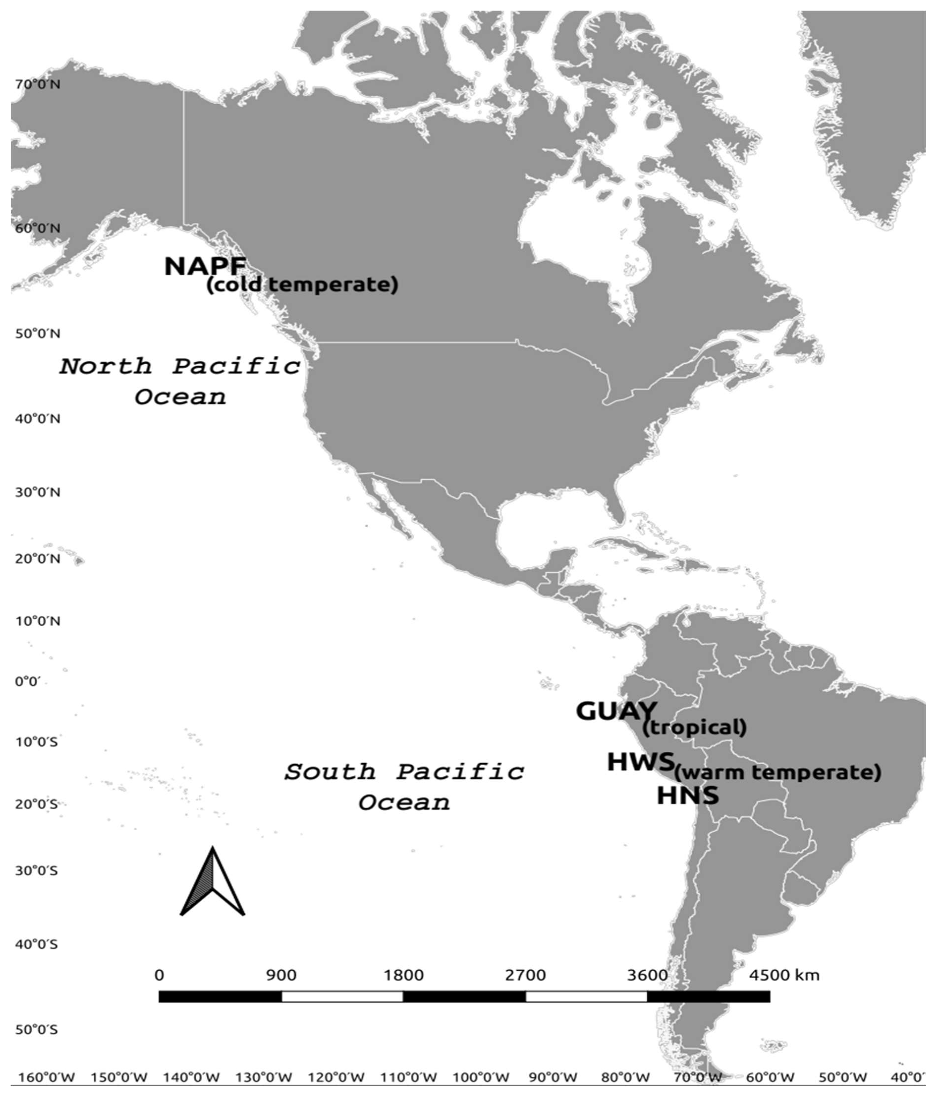

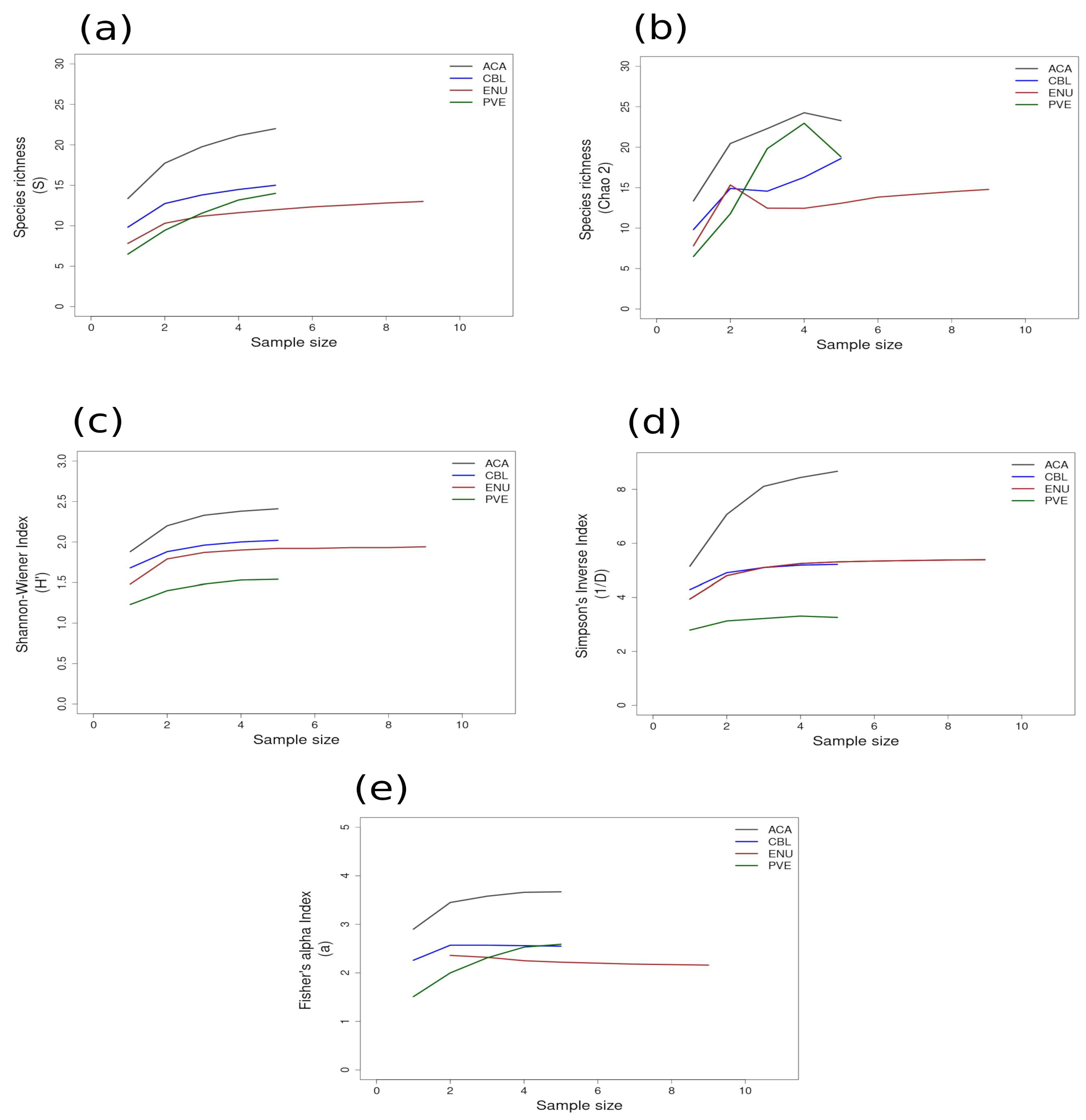
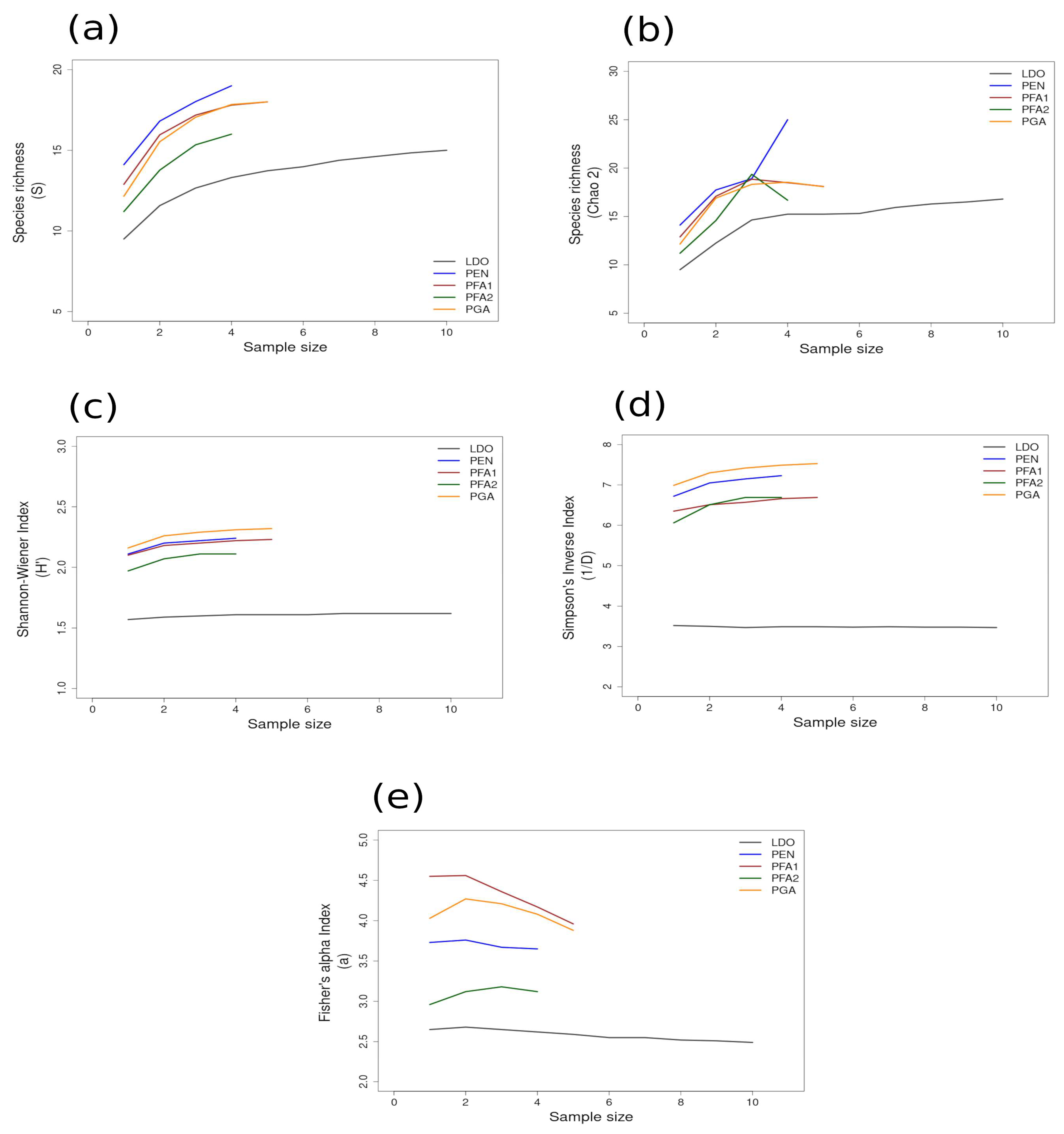
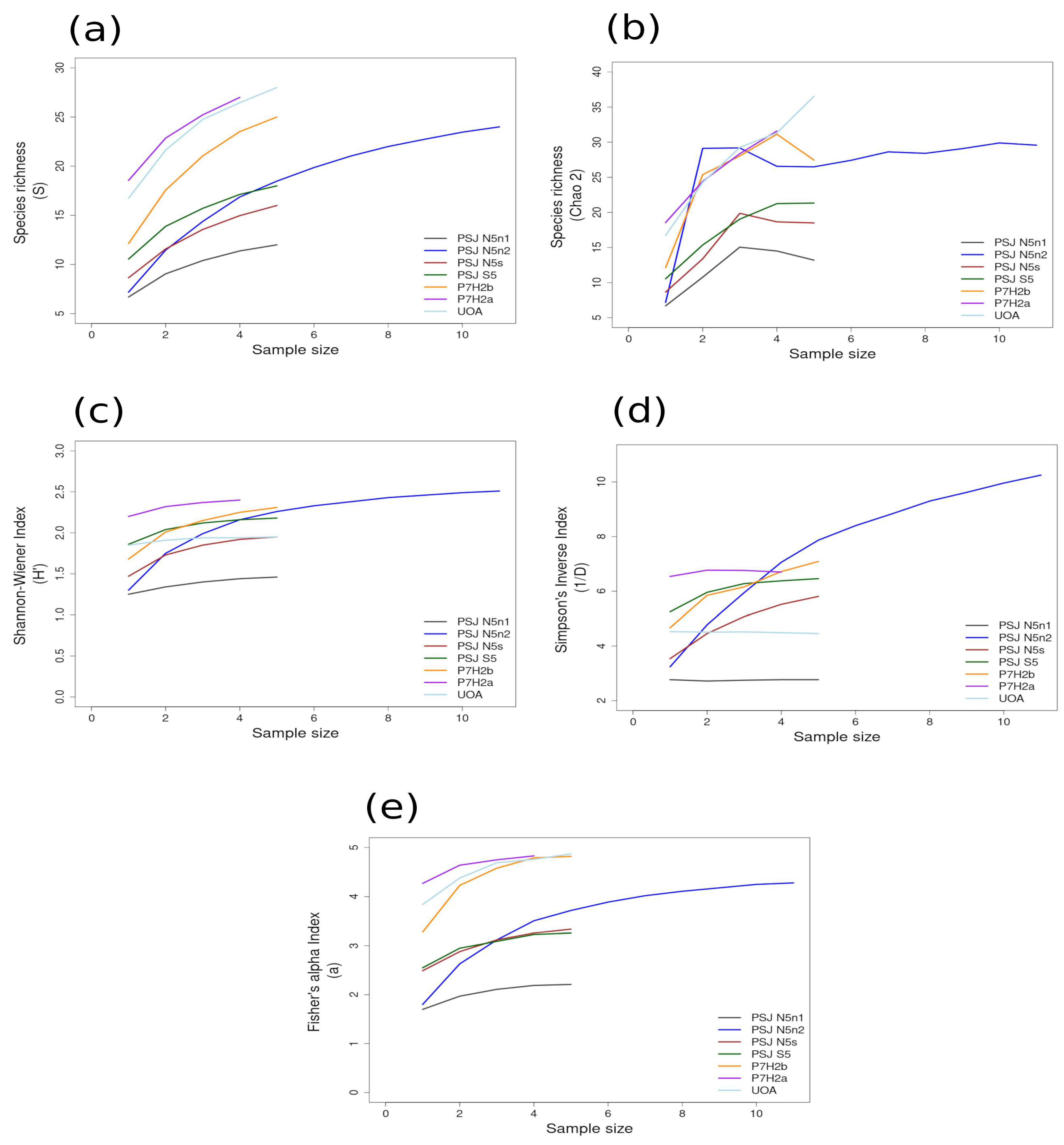
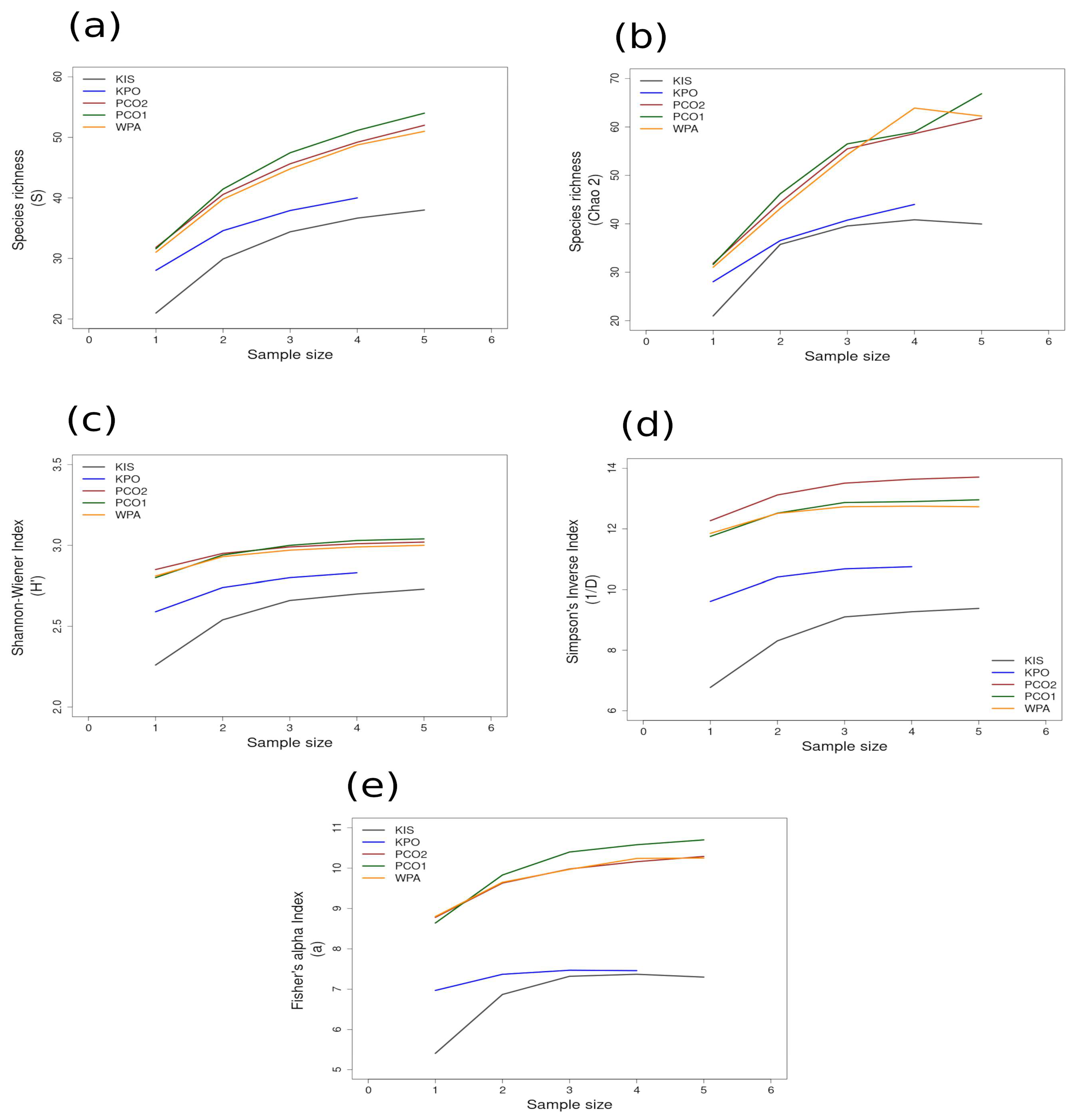
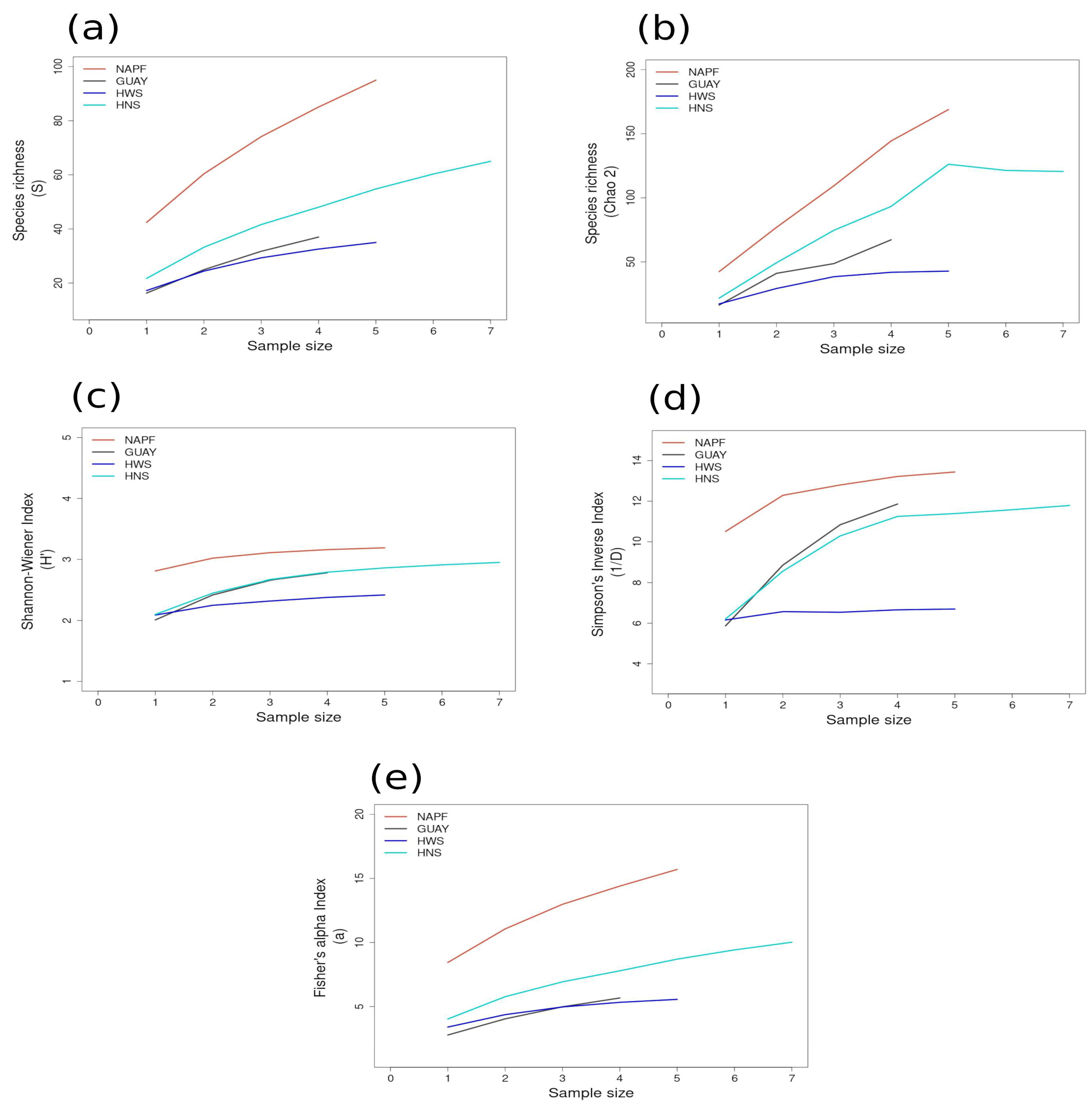
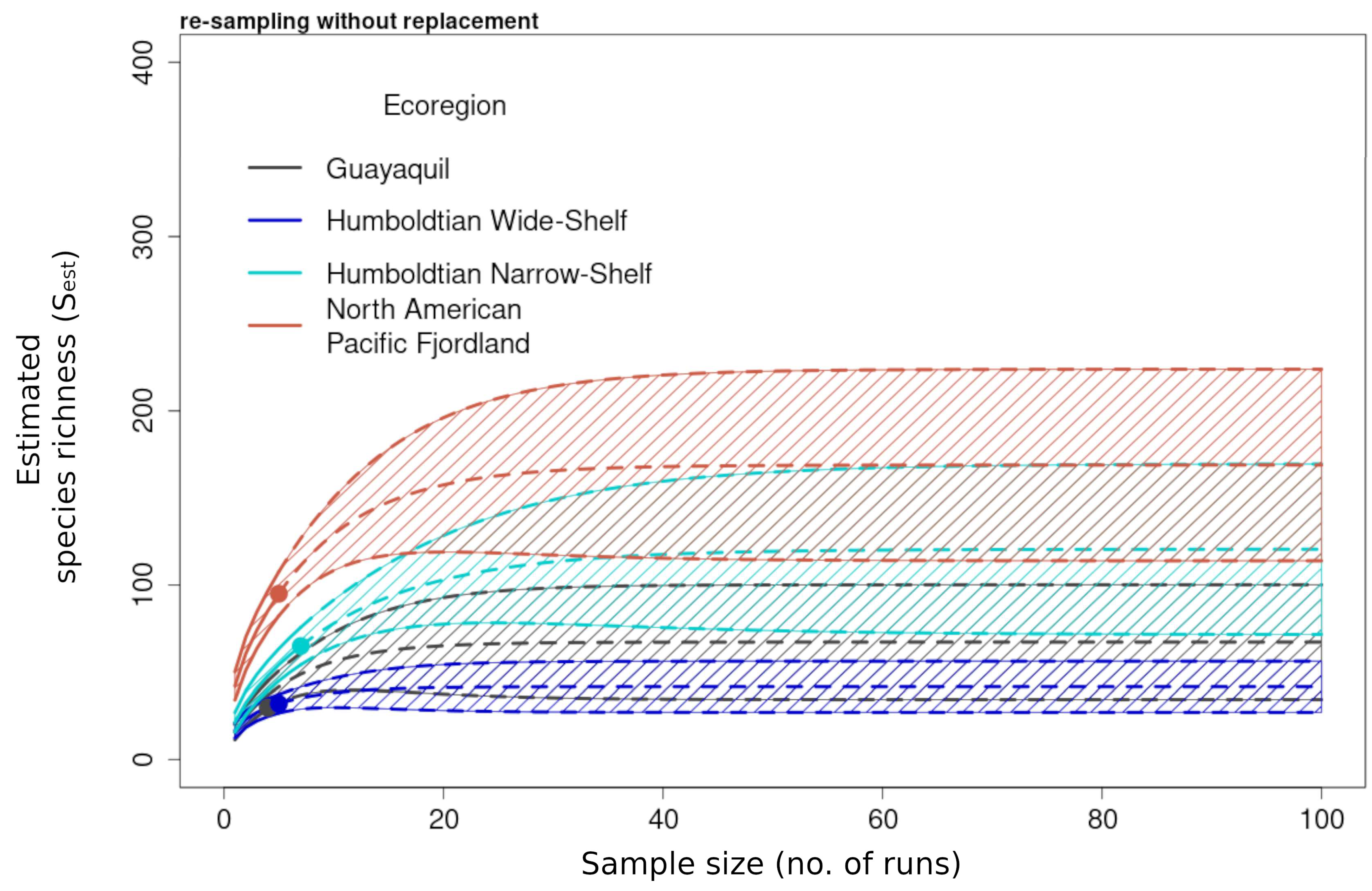
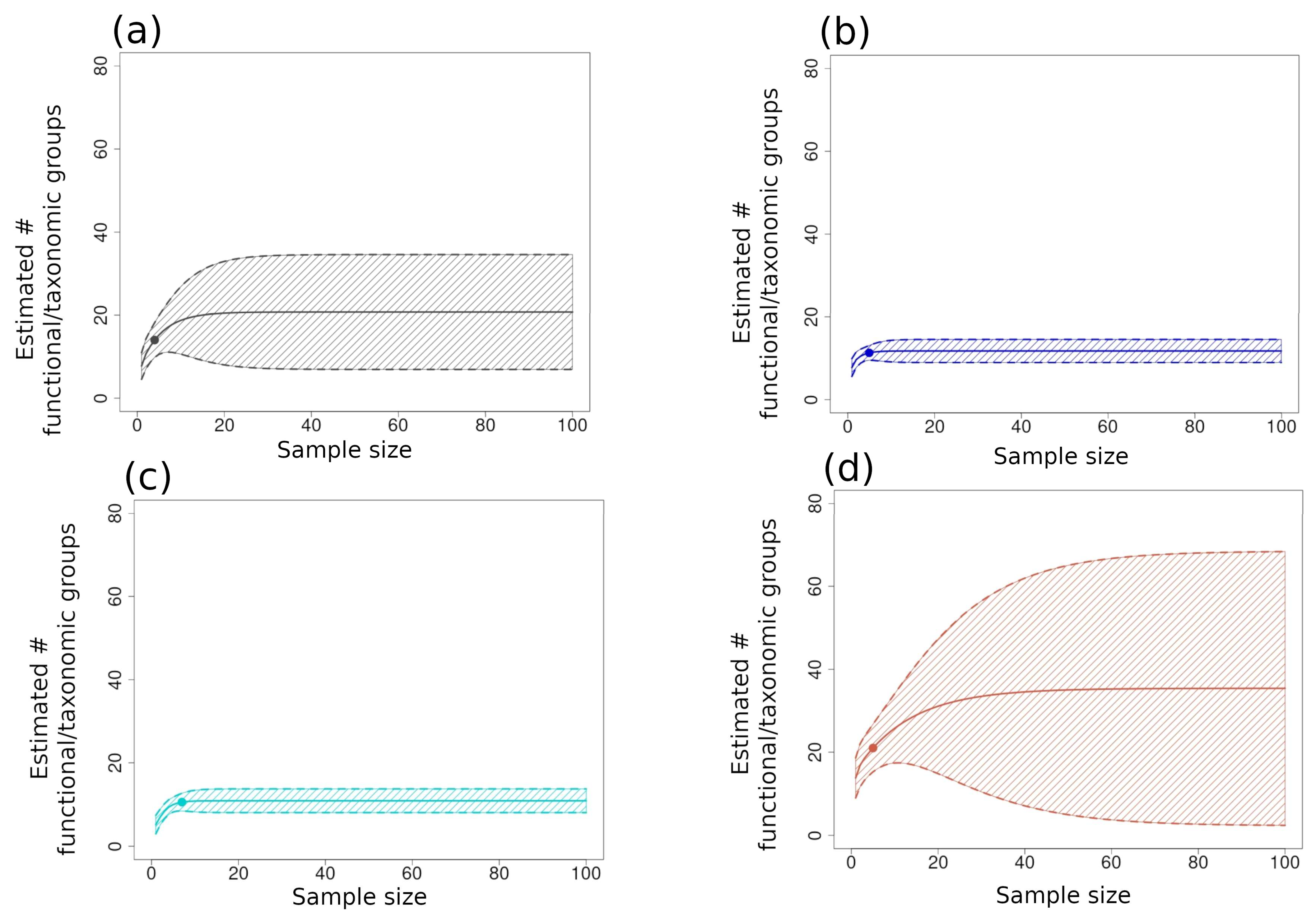
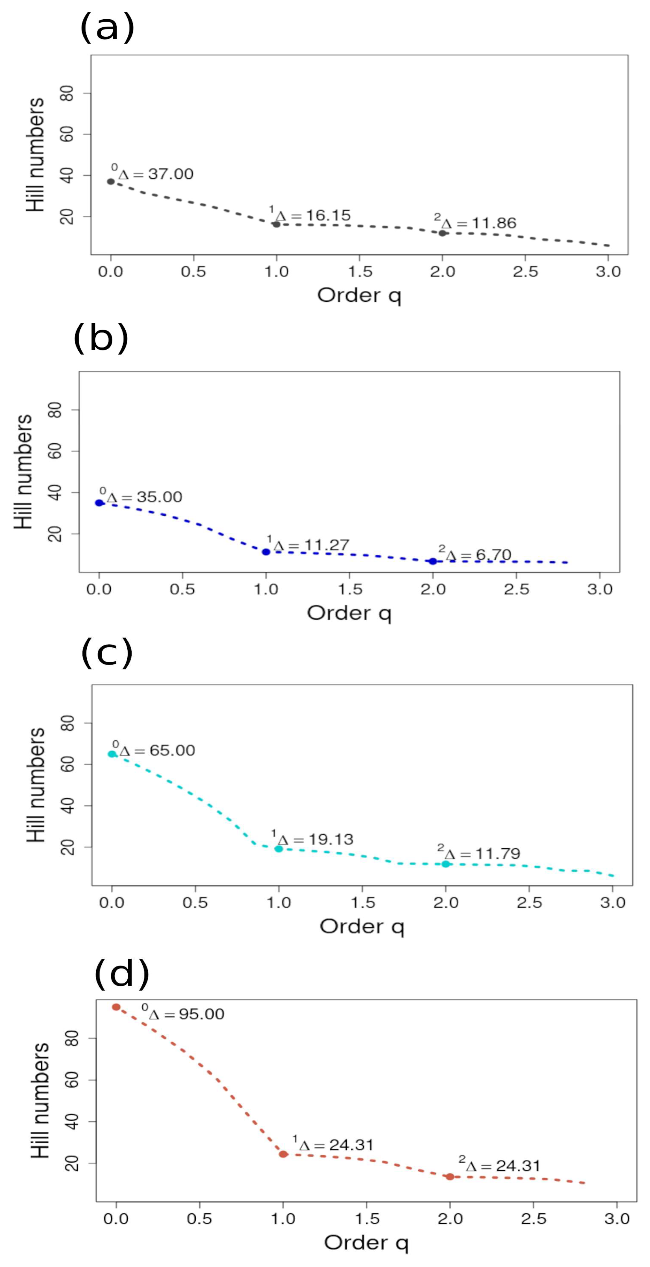
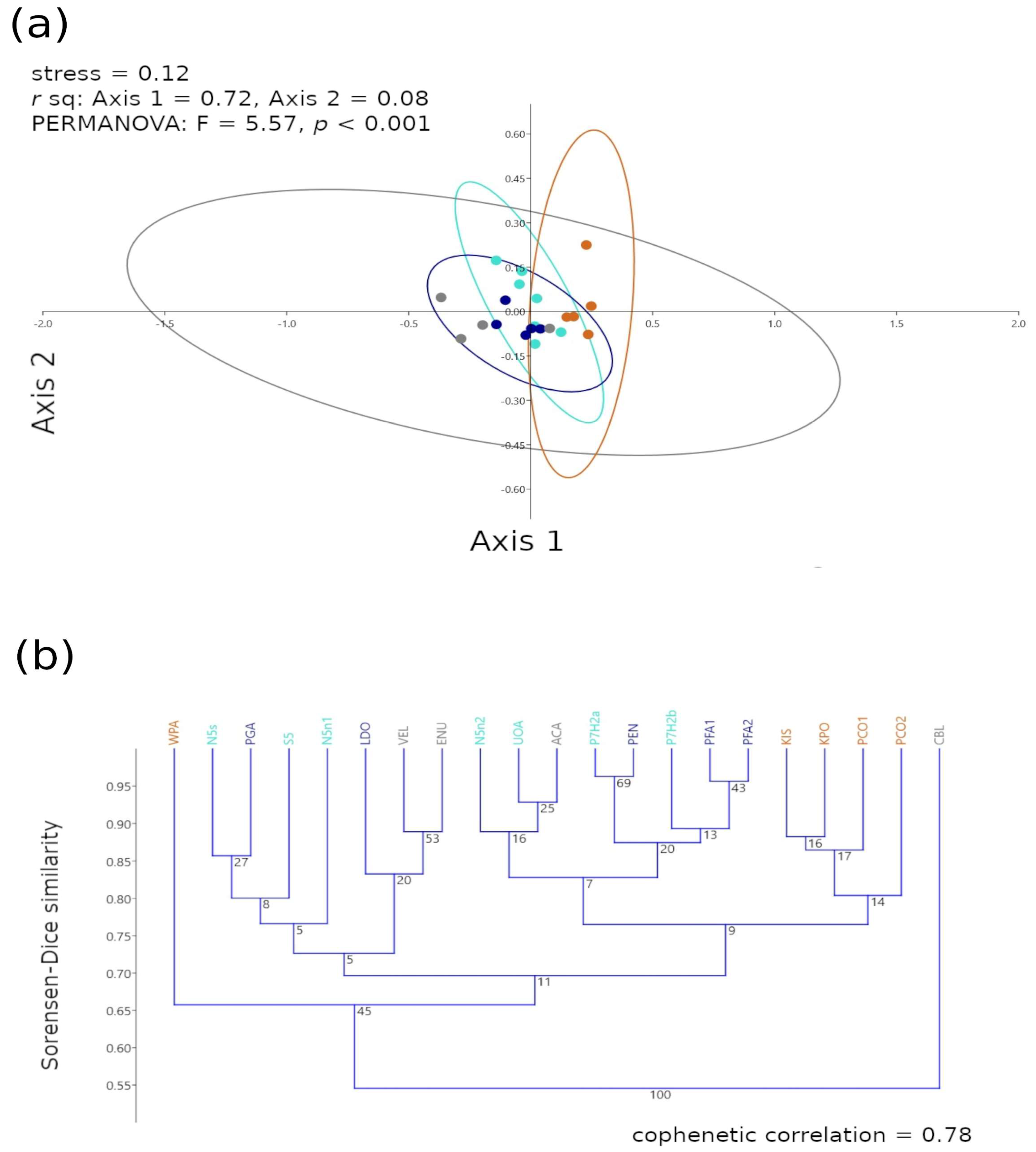

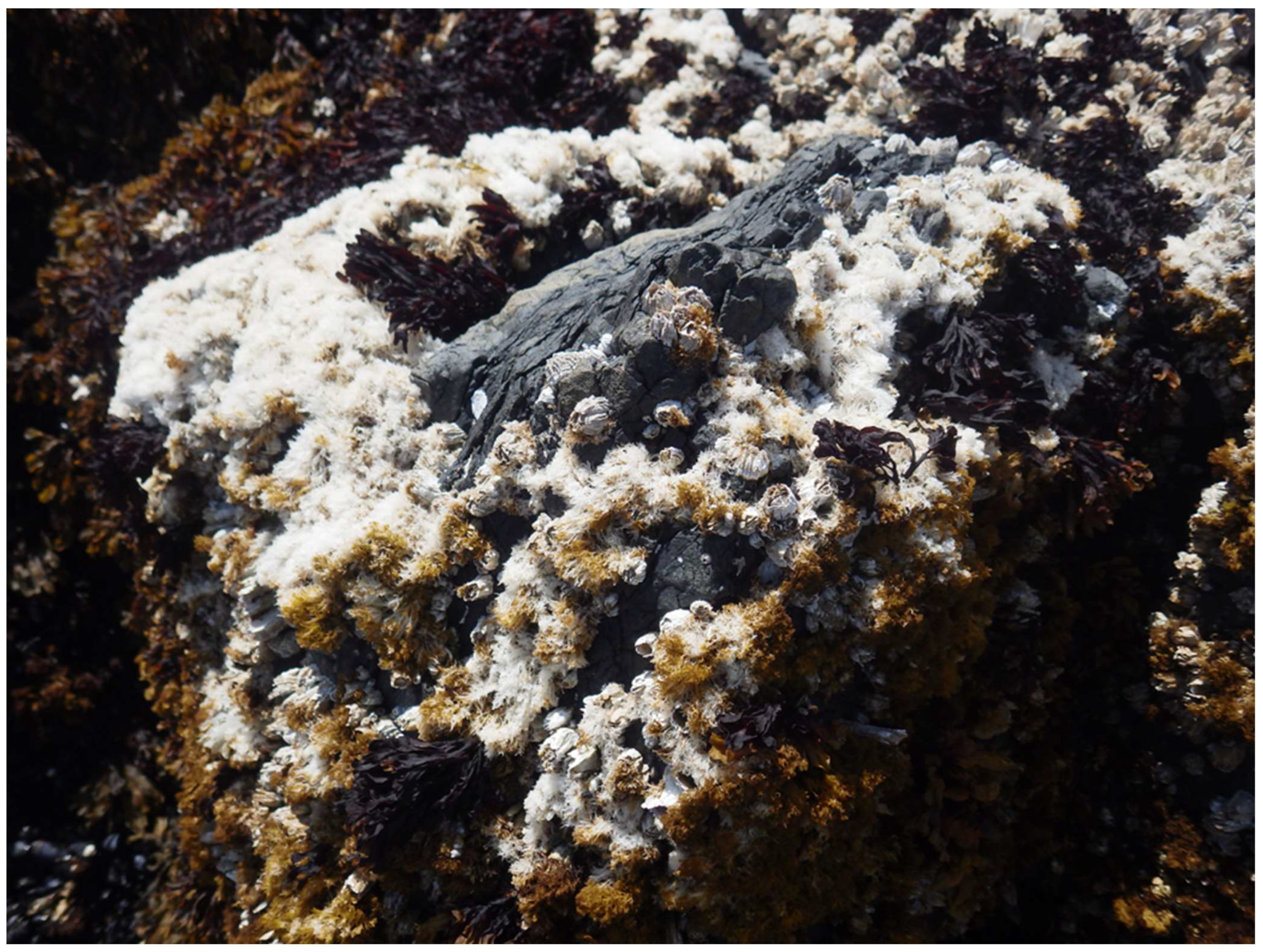
Disclaimer/Publisher’s Note: The statements, opinions and data contained in all publications are solely those of the individual author(s) and contributor(s) and not of MDPI and/or the editor(s). MDPI and/or the editor(s) disclaim responsibility for any injury to people or property resulting from any ideas, methods, instructions or products referred to in the content. |
© 2024 by the authors. Licensee MDPI, Basel, Switzerland. This article is an open access article distributed under the terms and conditions of the Creative Commons Attribution (CC BY) license (https://creativecommons.org/licenses/by/4.0/).