Article

Zooplankton of Bahía de Los Ángeles (Gulf of California) in the Context of Other Coastal Regions of the Northeast Pacific

by
Bertha E. Lavaniegos
*,
Guillermo Ortuño-Manzanares
and
José Luis Cadena-Ramírez
Department of Biological Oceanography, Centro de Investigación Científica y de Educación Superior de Ensenada (CICESE), Carretera Ensenada-Tijuana No. 3918, Zona Playitas, Ensenada 22860, Baja California, Mexico
*
Author to whom correspondence should be addressed.
Diversity 2025, 17(5), 316; https://doi.org/10.3390/d17050316
Submission received: 4 March 2025 / Revised: 16 April 2025 / Accepted: 17 April 2025 / Published: 27 April 2025

Abstract

:
Bahía de Los Ángeles (BLA) is located on the peninsular coast of the Gulf of California, near to the midriff islands. It is a greatly diverse ecosystem and a marine protected area due to its importance for whale sharks, turtles, and reef fishes. The bay also supports commercial fisheries that require ecological information for the integrated management of resources. Zooplankton studies are required as is an essential link in the trophic webs. There are few zooplankton studies in BLA focused mainly on the major taxa and species of copepods and cladocerans. Only one study addressed the seasonal variation in zooplankton but with gaps in the sampling. Here, we report the monthly changes in the zooplankton abundance and the composition of the major groups and cladoceran species. Eighty-one samples were collected between September 2017 and January 2019. The holoplankton taxa identified numbered 17, which accounts for 93% of the mean abundance (range 71–100%), with copepods and cladocerans being dominant. The meroplankton consisted of 15 taxa with a greater presence during the warm months (summer–autumn), dominated by the larval stages of bivalves, gastropods, and barnacles. In contrast, many copepod nauplii were found in January associated with low temperatures. Only cladacerans were identified to the species level. They showed strong seasonal fluctuations, reaching a third of the total zooplankton from spring to autumn, with Penilia avirostris being the most abundant species. These results are compared with other temperate and tropical coastal locations of the eastern Pacific.

Graphical Abstract

1. Introduction

The first faunal records of Bahia de Los Ángeles (BLA) came from scientific expeditions to the Gulf of California carried out at the end of the 19th century and the first half of the 20th century [1]. Among the numerous expeditions that entered the Gulf of California (GC), the campaigns led by Alexander Agassiz between 1891 and 1911 aboard the ship, Albatross (of the U.S. Fish Commission), stand out as part of a broader itinerary in the Eastern Tropical Pacific (ETP). The Albatross campaigns marked a milestone in the oceanographic research in the Pacific, with the collection of a substantial amount of pelagic and seafloor specimens and hydrographic data both in shallow areas and in deep basins [2]. These campaigns resulted in the first reports on the zooplankton in the GC and other regions of the ETP, on several crustacean groups (caridean decapods, mysids, euphausiids, copepods, and ostracods), and medusae [3].
Other expeditions, among the many that brought visibility to the GC, deserve special mention, such as the cruises of the ship, Velero III, carried out between 1931 and 1940, sponsored by the Allan Hancock Foundation; also the campaign organized by the New York Academy of Sciences in 1936, commanded by Templeton Crocker on his yacht (schooner Zaca); and the notable expedition of Steinbeck and Ricketts in 1940 [4]. In most of these expeditions, greater importance was given to the fishes, benthic macroinvertebrates, and terrestrial fauna of the islands. However, some plankton collections were made, which represent the first records of phytoplankton and some few zooplankton groups. Later, there were several cruises to the GC during 1956–1957 by the California Cooperative Oceanic Fisheries Investigation program, which led to a publication on the distribution, abundance, and biogeography of zooplankton taxa as medusae, siphonophores, chaetognaths, euphausiids, and pelagic amphipods [3].
Although some GC expeditions passed through BLA on their routes, the research focusing on the bay and the Ballenas Channel region really took off with the establishment of the Vermilion Sea Field Station by the San Diego Museum of Natural History during the years 1960–1972. The Vermilion station was established in the facilities of an old mine, conditioning them to carry out field activities and organize expeditions to the region of the large islands of the GC [5]. This effort produced interesting research on the hydrography, bathymetry, and sedimentology of BLA [6]. Concurrently with this survey, benthic sampling was carried out to determine the species composition of mollusks and their distribution [7], as well as polychaetes [8] and amphipods [9]. In these first investigations, sampling with nets to collect zooplankton was not contemplated.
The first BLA zooplankton study was conducted in 2007 by Nelson and Eckert [10], who collected samples with a conical net to document the feeding ecology of the whale shark (Rhincodon typus). They identified zooplankton at the level of major taxonomic groups, finding that copepods were by far the most abundant and the main prey of the whale shark. Other abundant groups included cladocerans and a variety of meroplankton, mainly the larvae of barnacles, decapods, bryozoans, echinoderms, and fish. Subsequently, Lavaniegos et al. [11] studied the seasonal variation in zooplankton in BLA based on quarterly sampling. Copepods were dominant, reaching 83–99% of the total zooplankton during the winter and spring, but could decrease in the summer and autumn between 25 and 66% due to the increase in cladocerans and meroplankton. These authors reported for the first time the species composition of copepods and cladocerans of BLA. The most abundant copepods during the winter were Calanus pacificus and Acartia tonsa, while in the summer, an increase in tropical species was observed (Centropages furcatus, Subeucalanus subcrassus, Acrocalanus longicornis, Temora discaudata, and Corycaeus amazonicus). The cladocerans Pseudoevadne tergestina and Penilia avirostris increased in summer–autumn. Some meroplanktonic groups, mainly echinoderm larvae, were abundant in the autumn in contrast to their scarcity in other seasons [11]. The high abundance of meroplankton during the autumn was corroborated by Hernández-Nava and Álvarez-Borrego [12] for the El Rincón area, where they constituted 63% of the zooplankton. The main motivation to research the zooplankton of BLA has been its trophic role in the feeding ecology of the whale shark. A recent study by Villagómez-Vélez et al. [13] used fatty acids as biomarkers to compare the lipid content of zooplankton and the stomach content and tissues of the whale shark. The high similarity between the fatty acid profiles of zooplankton and the liver of the whale shark are consistent with zooplankton-based nutrition.
Given the ecological importance of zooplankton in coastal marine ecosystems, a deeper understanding of the spatial and seasonal variability in BLA zooplankton is necessary. In the present study, we will return to the topic of seasonal variation in zooplankton groups and Cladocera species, based on the monthly sampling during 2017–2019. Likewise, it seeks to elucidate whether there are differences between the sites within the bay. Multivariate analyses will be used to compare the spatiotemporal differences during the study period with the previous data from 2003–2004 taken from Lavaniegos et al. [11].

2. Materials and Methods

2.1. Study Area

Bahia de Los Ángeles is in the middle part of the eastern coast of the Gulf of California, with wide communication with the Ballenas Channel, which provides the bay with cold water and strong currents [14]. BLA includes a chain of small islands and three deep but gently sloping channels. One of them is between Coronado Island and the peninsular coast, another one is south of Coronado Island, and the third one is between Cabeza de Caballo Island and the coastline between Punta Roja and Puerto Don Juan (Figure 1). The climate of BLA is arid and extreme, with little rainfall [15]. The average annual atmospheric temperature is 22.7 °C with the maximum during July–August (>35 °C) and minimum during January–February (<11 °C) [15].
BLA is dominated by the Gulf of California water mass, with high salinity (≥35 psu) due to evaporation [16]. The tides are intense and generate currents in the Ballenas Channel [17] and between the straits and the numerous islands of BLA, producing nutrient mixing and high productivity [18]. The variation in the sea level due to the tides induces gentle currents intensified by the winds [14]. Northwesterly winds induce particularly intense upwellings during the winter in the Ballenas Channel that enrich the surface waters and allow the development of phytoplankton blooms [19] and a high incidence of red tides [6,20]. The phytoplankton biomass produced in the Ballenas Channel is partially exported to nearby bays such as BLA [21]. Later studies have confirmed high rates of primary productivity in the bay [20,22,23].
There are many biotopes in the Gulf of California. Parker (1964) considered twelve types of environments in the GC [24] depending on the depth, type of substrate, water temperature, and oxygen concentration. BLA corresponds to the intertidal rocky environment, typical of the peninsular coast of the gulf. However, BLA also presents sandy and silty planes, especially in the southern portion where the bay is shallower [6]. In the northern region of the bay and around the numerous islands, the rocky substrate is predominant, and the calcareous accumulations are produced by mollusks, bryozoans, echinoderms, and corals [25].

2.2. Zooplankton Sampling and Identification

Zooplankton samples were collected at seven locations in the inner part of BLA, between the Baja California peninsula and the archipelago (Figure 1). In 2017, two samplings were carried out (5 September and 21 October), with monthly samplings between March 2018 and January 2019. All the samplings were carried out in the morning using a conical net with a 50 cm diameter mouth and 200 µm mesh size. The net was towed superficially for five minutes at an approximate speed of 3 km h−1. The volume of filtered water was measured using a flowmeter placed at the mouth of the net. The material collected by using the net was fixed with 4% formaldehyde.
In the laboratory, organisms were identified and counted in a fraction (½–⅛) of or the entire sample depending on the quantity of plankton in the sample. The major taxonomic groups were identified with a stereomicroscope Wild Heerbrugg (Switzerland) using coastal zooplankton identification guides produced by Yamaji [26] and Todd and Laverack [27] and the atlas of marine invertebrate larvae edited by Young et al. [28]. Only cladocerans were identified to species or genus level with reference to Onbè [29].

2.3. Temperature Data

The surface temperature was recorded using a thermometer. Additionally, temperature data from the Operational Sea Surface Temperature and Sea Ice Analysis (OSTIA) system were used, available at https://seatemperature.info/es/bahia-de-los-angeles-temperatura-del-agua-del-mar.html (accessed 12 April 2020). These forecasts are based on a combination of satellite records provided by international agencies and the available databases [30].

2.4. Data Analysis

The abundance of organisms found in the sample was divided by the volume of water filtered via the net and is reported as individuals per cubic meter (ind m−3). The monthly variation in the abundances of different groups and species is described. Agglomerative clustering analysis was used to compare the similarity of the zooplankton community between the sampling months and sites. The taxonomic groups present in >10% of the samples were considered, resulting in a matrix of 31 taxa x 86 samples. The abundance data for the different zooplankton groups were transformed using the function xi = log (x + 1). A similarity matrix was then calculated using the Bray–Curtis index. A dendrogram was constructed using a flexible beta of −0.25 as the cluster amalgamation procedure. The dendrogram was cut at a threshold of 65, and the differences between the resulting clusters were analyzed using pairwise ANOSIM statistics. These procedures were performed using the PRIMER 7 software [31]. The contribution of each species to the similarity of the clusters was determined using the SIMPER routine.
Additionally, the abundances of zooplankton groups from 2017 to 2019 were compared with published data from 2003 to 2004 taken from a previous study by Lavaniegos et al., 2012 [11]. For this purpose, only analogous sampling dates and seasons were considered in both studies, so it was only possible to compare three seasons (spring, summer and autumn) from four sampling sites (LG, PA, PR, and ER). Firstly, univariate comparisons were carried out by taxonomic groups using the non-parametric Kruskal–Wallis rank test. A multivariate analysis of similarity between zooplankton communities was subsequently performed. For this purpose, a similarity matrix was calculated in the same manner as described above. Then, a non-metric multi-dimensional scaling ordination (NMDS) was carried out. The threshold value used to slice the clusters in the NMDS was 50, and the differences among them were tested using ANOSIM.

3. Results

3.1. Surface Sea Temperature

The range of sea surface temperature (SST) during the sampling period was 15.7–28.2 °C, corresponding to the average recorded during March and July 2018, respectively. In May, a higher SST (21 °C) was observed in the southeast of the bay, at the stations El Rincón (ER) and Punta Roja (PR), while in the rest, it was 17–18 °C (Figure 2a). This is because the southeast region is protected from the northwesterly winds typical of the spring [14]. However, in July, the SST increased rapidly and was more homogeneous between the stations (27–29 °C). In the summer, the wind changes from the east to west [14]. Now, the stations located southeast of BLA are the most exposed, and this explains a rapid cooling at the end of the summer in ER and PR. During autumn–winter, the SST was homogeneous throughout the bay, with a drastic cooling between October and November.
The SST measured in situ was near to that reported by the OSTIA program, based on satellite data. However, some notable differences were observed (Figure 2b). For example, on 8 May 2018, the SST measured in situ was 20.4 ± 0.9 °C while it was warmer than that as estimated with reference to the satellite data (17 °C). Shortly after, on 29 May, the temperature of BLA decreased and behaved more in accordance with the satellite data. In contrast, on 2 September, the measured SST was lower (25.6 ± 1.2 °C) than the satellite data (28 °C), indicating that the seasonal temperature drop began in September. Also, a SST 2.5 °C lower than the satellite data on 3 December shows that the actual temperature drop is more abrupt towards the end of autumn.

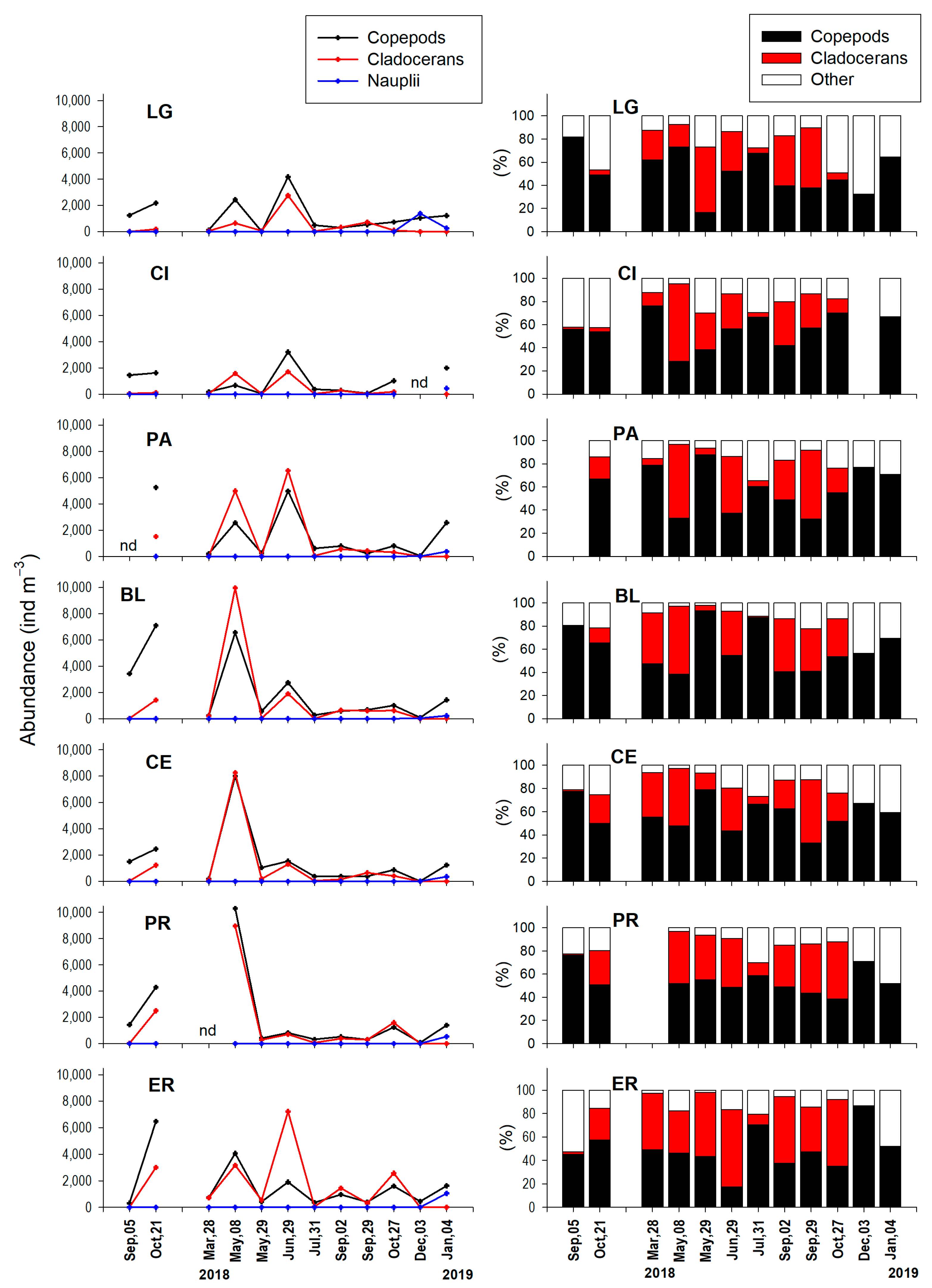
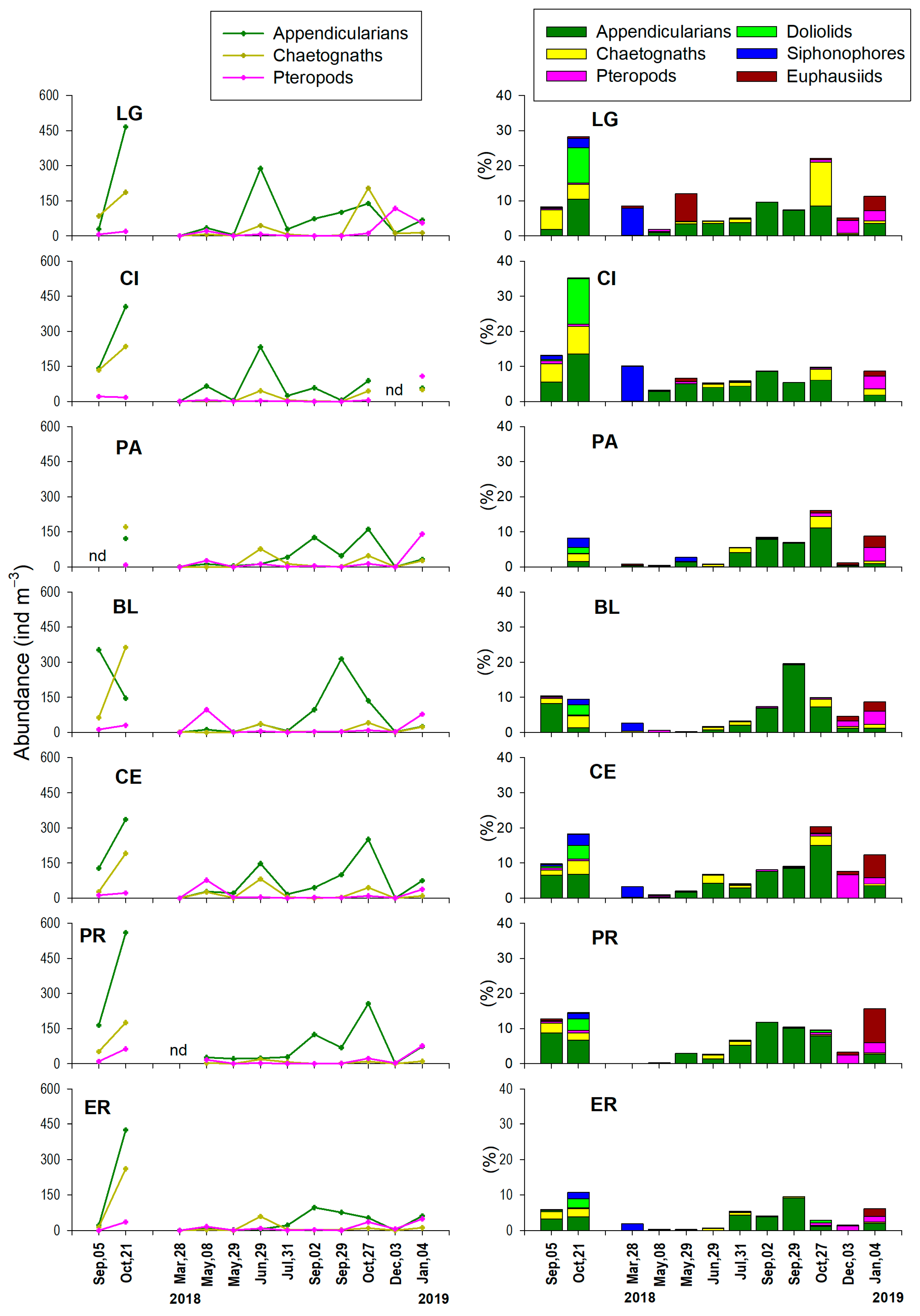
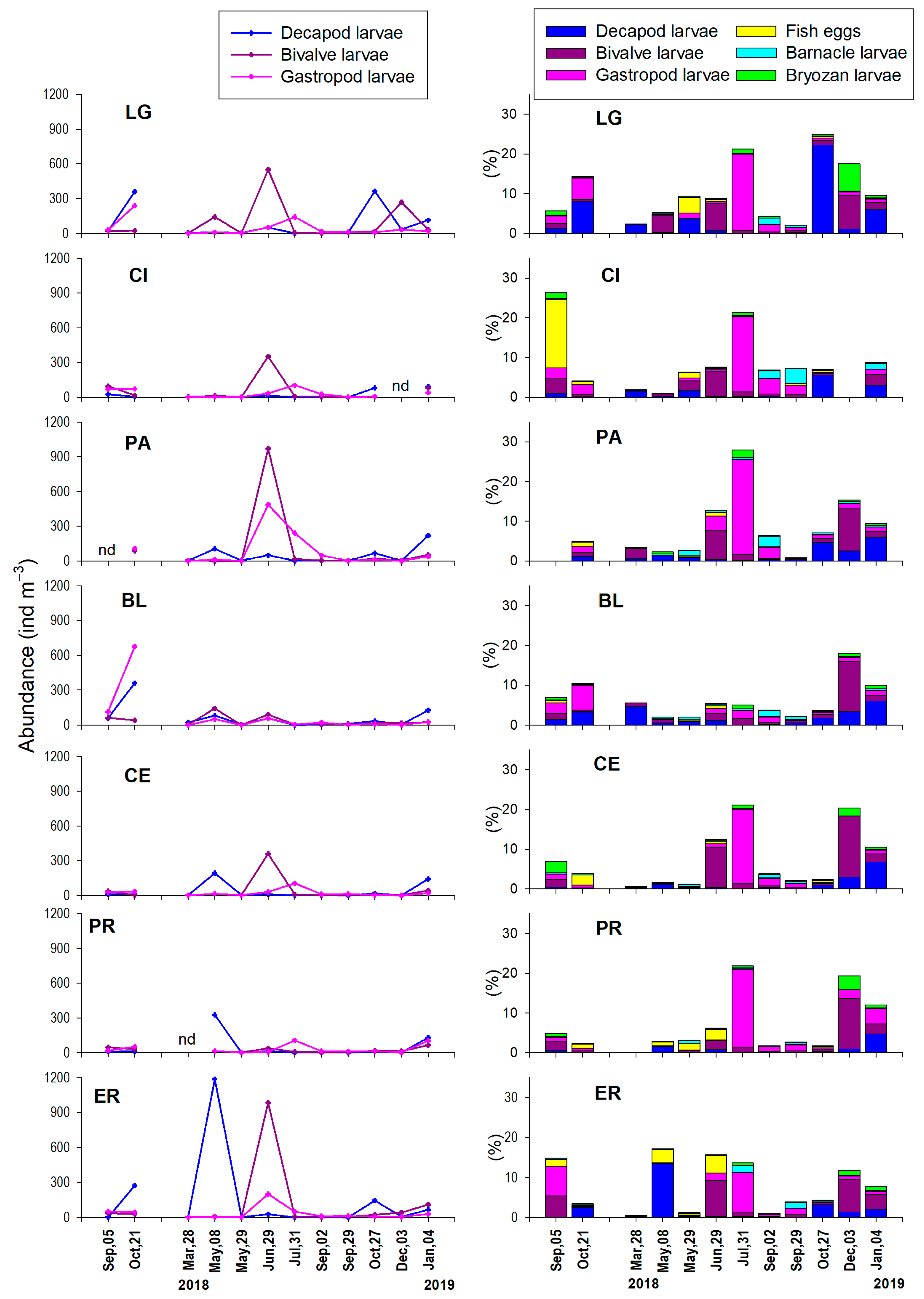
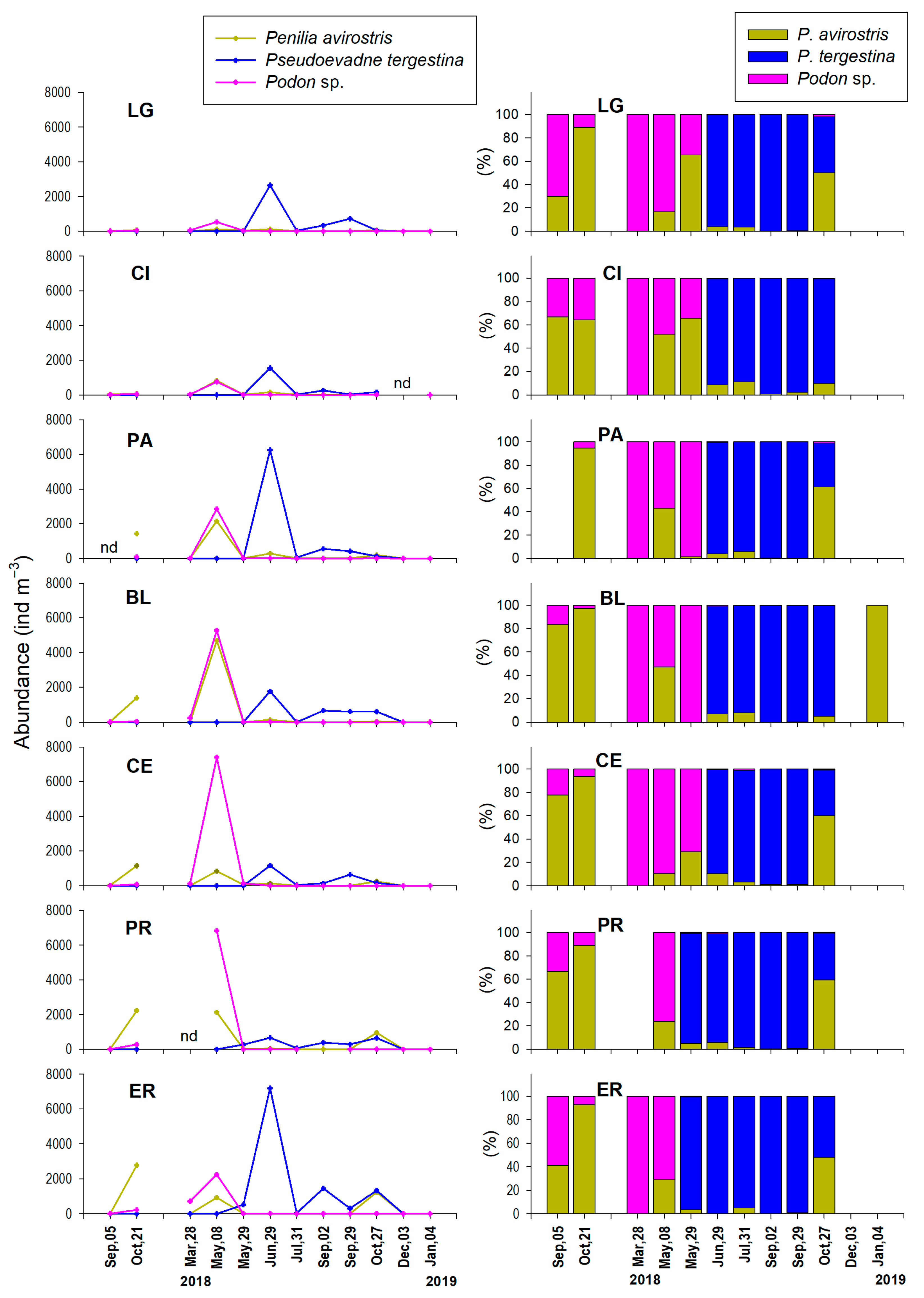
3.2. Major Zooplankton Taxa

The zooplankton found in the samples included 19 holoplankton taxa from eight different phyla (Table 1). The detailed abundance of taxonomic groups for each station can be consulted in Supplemental Table S1. The most abundant were two groups of crustaceans (copepods and cladocerans), found in 100% and 85% of the samples, respectively. Other frequent holoplanktonic groups were appendicularians (98%), polychaetes (89%), chaetognaths (84%), and pteropods (83%). On the other hand, foraminiferans, hydromedusae, siphonophores, heteropods, amphipods, euphausiids, doliolids, and salps were less frequent (21–57%). Nauplius larvae (16%) were also considered within the holoplankton, since they mostly corresponded to copepod nauplii. Some pelagic decapods (carids and penaeids) were found but not counted separately from the meroplanktonic decapod larvae, so this group will be considered within the meroplankton from now on. The least frequent holoplankton groups (<10%) were ctenophores, ostracods, and mysids.
The abundance of all holoplankton was between 71 and 100% in the samples, with a mean of 93%, while that for meroplankton was 7% (range: 0–29%). Due to the shallow depth of the bay and the presence of macroalgae, some benthic elements were captured in the net. Isopods and platyhelminthes were the most common, being present in 30% of the samples. Nematodes, cephalochordates (Branchiostoma), and cumaceans were found in <5%. The meroplankton groups corresponded to the larvae of twelve different phyla (Table 1). The most frequent were bivalve and gastropod mollusks (99% and 93%, respectively), and the most common crustaceans were cirripedians (97%) and decapods (75%). Fish eggs occurred in 80% of the samples. The larvae of bryozoans, echinoderms, and fish were of regular frequency (51–74%), while the larvae of polychaetes, stomatopods, phoronids, nemerteans, and sipunculids were less frequent (22–30%). The rarest larvae (<13%) were those of cnidarians, hemichordates, and brachiopods.

3.3. Monthly Variability of Zooplankton

3.3.1. Holozooplankton

The most abundant groups of zooplankton were copepods and cladocerans, which showed seasonal fluctuations and differences between the sampling sites (Figure 3). The highest abundances of copepods were observed in early May 2018 at stations PR, CE, and BL, with values higher than 6000 ind m−3. High abundances of copepods were also observed at BL in October 2017, as well as at two shallow stations in the south of the bay (PA and ER). However, they were not abundant in October 2018. The northern stations (LG and CI) were poor in copepods throughout the year, with abundances ranging from 19 to 4178 ind m−3. The nauplii abundance is also shown in Figure 3. They were relatively large nauplii and could therefore be retained by using the net and were only observed in the winter. The maximum nauplii abundance was 1383 ind m−3 in LG during December and 1042 ind m−3 in ER during January. In relative terms, copepods had a wide range (17–93%), but the average was 55% of the total zooplankton. The decrease in the relative abundance of copepods was mainly due to the increase in cladocerans. These constituted between 23 and 38% during the spring, summer, and autumn, while they were absent in the winter. The rest of the zooplankton represented a very variable fraction (2–67%), but on average, it was 36% in the winter and 9% in the spring (Figure 3).
After copepods and cladocerans, the most abundant holoplankton groups were appendicularians, chaetognaths, and pteropods, which showed a different seasonal trend, increasing in the autumn or winter. Appendicularians were present all year round in BLA (Figure 4), but their highest abundance was in the autumn, reaching 6–10% of the total zooplankton. Chaetognaths reached approximately 4% of the total zooplankton during the autumn, while the rest of the year they were <1% (Figure 4). Pteropods increased in the winter with an abundance ranging 38–141 ind m−3, representing around 3% of the zooplankton. However, at some stations (BL and CE), a peak was observed in the spring (97 and 77 ind m−3, respectively) but in percentage terms was barely perceptible (<1%) given the high abundance of copepods and cladocerans (Figure 4).
Euphausiids were another frequent group (50% of the samples) but with a generally low abundance. During 2017–2018 the euphausiid abundance had a monthly mean of less than 8 ind m−3 increasing only in January 2019 (107 ind m−3). These were larval stages probably due to the morning sampling schedule, since juveniles and adults perform circadian vertical migrations. Similarly, doliolids and siphonophores had low abundances except for October 2017 with monthly means of 290 and 144 ind m−3, respectively. The density of doliolids was higher at stations LG and CI while that of siphonophores was higher at stations located in the southern part of the bay. The combined relative abundance of euphausiids, doliolids, and siphonophores averaged between 0.02 and 7.4% during the sampling period (Figure 4).
Some holoplankton groups were frequent (polychaetes, hydromedusae, foraminiferans, and heteropods), but their global mean abundance was, respectively, 6, 3, 3, and 1 ind m−3. Together, they averaged 0.02 and 5.6%. The least frequent groups were amphipods, salps, ctenophores, ostracods, and mysids, being absent in 75–94% of the samples. Note that ctenophores were found in high abundance (193 ind m−3) in one of the samples collected at the ER station during September 2017.

3.3.2. Meroloplankton

The zooplankton of BLA was rich in meroplanktonic forms. Among the crustaceans, the most abundant were decapods, mainly zoea and some crab megalopas. Their abundance varied between the stations, with several showing an increase in October 2017 (BL) or in both autumns (ER, LG). At stations located south of the bay, a peak in abundance was observed in the spring, with a maximum of 1185 ind m−3 at station ER (Figure 5). Other abundant meroplankton in BLA were the veliger larvae of bivalve and gastropod mollusks. The peak abundance of bivalve larvae occurred in June, reaching the maximum values in ER and PA (982 and 970 ind m−3, respectively). Gastropod larvae also showed a tendency towards higher abundances in the summer, being particularly high in PA. The only station with the maximum abundance in October 2017 was BL (Figure 5).
Together, decapod and mollusk larvae account for 2–19% of zooplankton. Other abundant meroplanktonic elements were fish eggs, barnacle larvae, and bryozoans, which constituted 0.2–5% of the zooplankton (Figure 5). Fish eggs showed differences in their abundance by location but without a seasonal trend. The same occurred with bryozoan cyphonautes larvae, with a specific increase (218 ind m−3) in LG during December 2018. In contrast, barnacle larvae had a more ubiquitous presence throughout the bay and a tendency to increase in spring–summer.
Echinoderm larvae were also frequent, being observed in 51% of the samples, but in low abundance (global mean = 5 ind m−3). Only during 2017 were they more abundant at stations BL, CE, and PR (20–45 ind m−3). Other invertebrate larvae (sipunculids, nemerteans, polychaetes, stomatopods, phoronids, cnidarians, brachiopods, etc.) were rare, representing between 0 and 3% of the zooplankton.

3.3.3. Cladoceran Species

Previously, it was stated that cladocerans had a markedly seasonal behavior, going from being one-third of the zooplankton from the spring to autumn until disappearing in the winter. In spring 2018, the first species recorded were Penilia avirostris and Podon sp. with high abundances in May 2018 (Figure 6). The high abundances of P. avirostris occurred at stations BL, PA, and PR (>2000 ind m−3). However, at other locations (CI and LG), the abundance remained below 1000 ind m−3 throughout the year. The dynamics of Podon sp. was similar with the maximum abundance at BL, PR, and CE (>5000 ind m−3).
The last species recorded during the sampling period was Pseudoevadne tergestina, peaking in abundance during June 2018. This species was associated with the warmest June temperatures in ER and PA with abundances >6000 ind m−3. In autumn 2018, it was also abundant, contrasting with its absence in the previous autumn of 2017 (Figure 6). The relative abundance of the three species further highlights the seasonal succession of P. avirostris and Podon sp followed by P. tergestina. It is also noted that P. tergestina emerged first in the southernmost stations (ER and PR) from May 2018, while in the rest of the bay, it did so until June 2018.

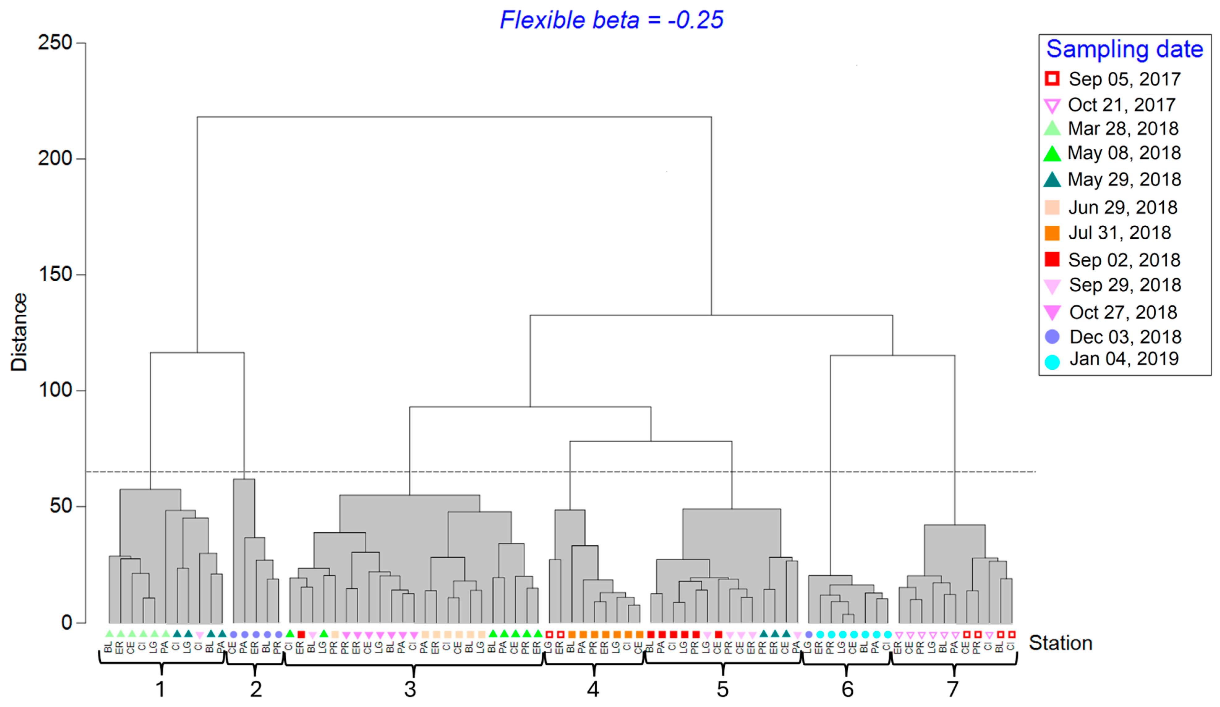
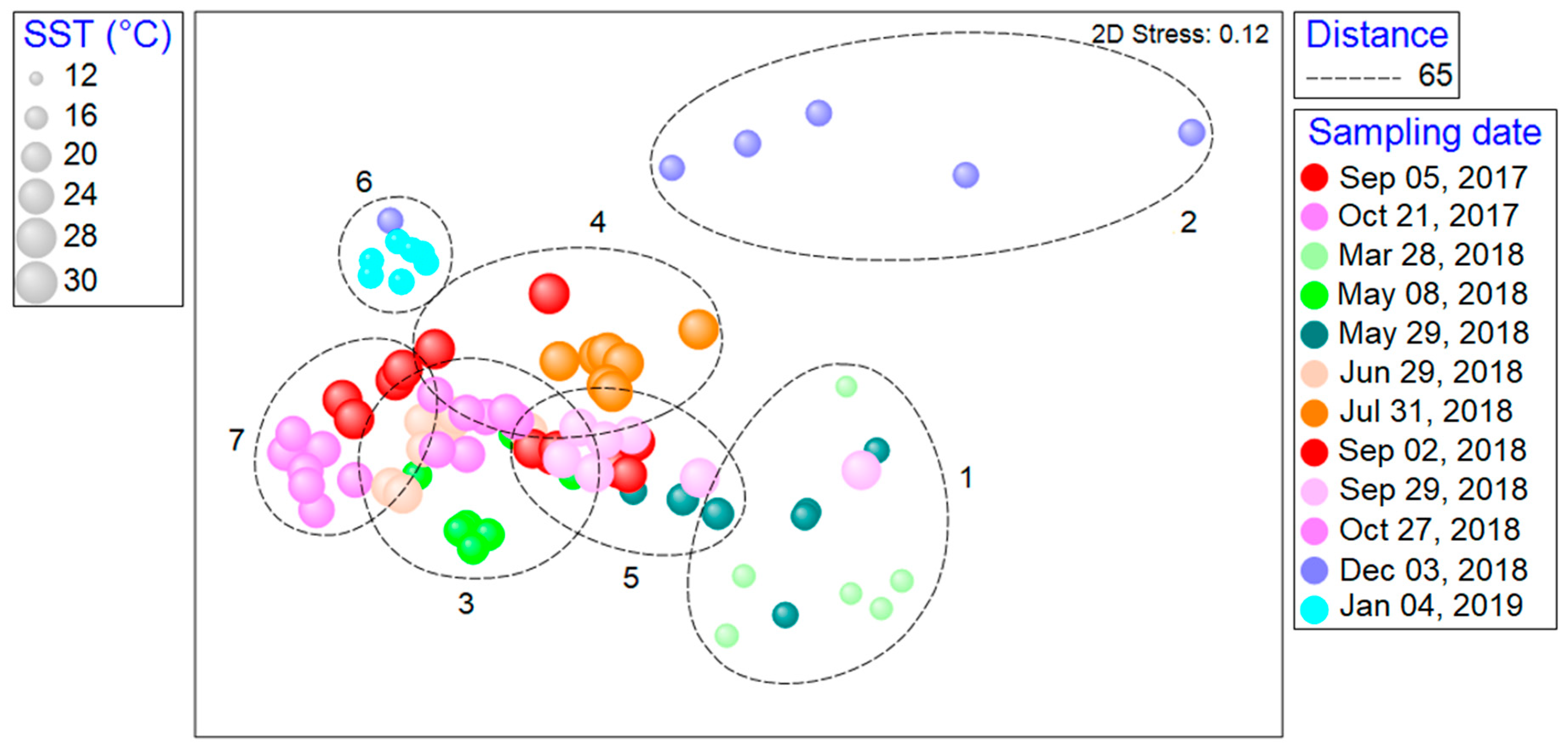
3.4. Space–Time Similarity of Zooplankton Communities

Multivariate analysis based on a similarity matrix is shown in Figure 7. Seven clusters were obtained considering a cutoff distance of 65. The ANOSIM test comparing these clusters showed significant differences, with an overall R of 0.854 (p = 0.01), and for all the possible pairwise comparisons (p < 0.03). The conglomerate marked 3 in Figure 7 was the largest, combining the sampling stations sampled on 29 May, 29 June, and 27 October 2018, along with a pair of September stations. It could be considered a characteristic assemblage of transition periods, with temperate–warm temperatures (Figure 8). The fact that it brings together all the stations from these three samplings indicates that the spatial differences are not considerable with respect to large taxonomic groups. The main contribution to similarity in cluster 3 was that of copepods, cladocerans, and appendicularians, which together accounted for 48% (Figure 9).
Most of the spring stations that fell outside of cluster 3 were grouped into cluster 1. The main difference between these clusters was due to cladocerans, which had a greater contribution to the similarity in cluster 1 (29%). Adding copepods and cladocerans together, the contribution was 68%. Adding copepods and cladocerans, the contribution of these groups was 68%. However, the zooplankton abundance was low, with a median of 241 ind m−3 for the stations in cluster 1. In contrast, in cluster 3, the median was 3508 ind m−3 (Figure 9A). The SST at stations in cluster 1 was low (15–18.2 °C), excluding one autumn station associated with this cluster (27 °C, Figure 8).
The majority of the 2017 stations, corresponding to late summer (5 September) and the autumn (21 October) were grouped in cluster 7 (Figure 7). A characteristic of this cluster was the lowest contribution of copepods to community similarity (12.5%), despite their notable abundance (Figure 9). The contribution of cladocerans was also low (7%), in the same order as appendicularians and chaetognaths. The latter had their highest abundances in cluster 7 compared to the other clusters (medians of 336 and 175 ind m−3, respectively). The summer samples predominated in clusters 4 and 5 (Figure 7). Cluster 4 included the stations from 31 July 2018, which, along with two stations from 5 September 2017, presented the highest SSTs (Figure 8). The taxa with the greatest contribution to the similarity of group 4 were copepods, gastropod larvae, and appendicularians, which together accounted for 48% (Figure 9B). In cluster 5, most of the samples corresponded to the summer (2 September), autumn (29 September), and three more from the spring (29 May). The main contributions were from copepods, cladocerans, and appendicularians (65%). The dissimilarity between clusters 4 and 5 was mainly due to cladocerans and gastropod larvae. The first showed an increase from July to September (from 35 to 354 ind m−3), while the second decreased drastically (from 103 to 11 ind m−3, Figure 9A).
Clusters 2 and 6 were the purest, grouping stations with low SSTs (16–18 °C; Figure 8). However, these clusters appear distant in Figure 7 despite their closeness in time (December and January). The biggest difference between both clusters was the abundance of zooplankton, very low in cluster 2 compared to cluster 6 (medians of 97 and 2827 ind m−3, respectively). Copepods made the greatest contribution to the similarity of their respective clusters but in different proportions (39.5% in cluster 2 and 12.5% in cluster 6). Another difference in similarity was the contribution of bivalve larvae, which was 21% in cluster 2 but only 8% in cluster 6. (Figure 9). Nauplii showed a high contribution to similarity (11% in cluster 2 and 12% in cluster 6), but their abundances were markedly different, with a median of 3 ind m−3 in cluster 2 and 400 ind m−3 in cluster 6.
Thus, this multivariate analysis of abundances by taxonomic group primarily points to temporal changes rather than between the sampling sites. The temporal differences observed were both seasonal and intra-seasonal.

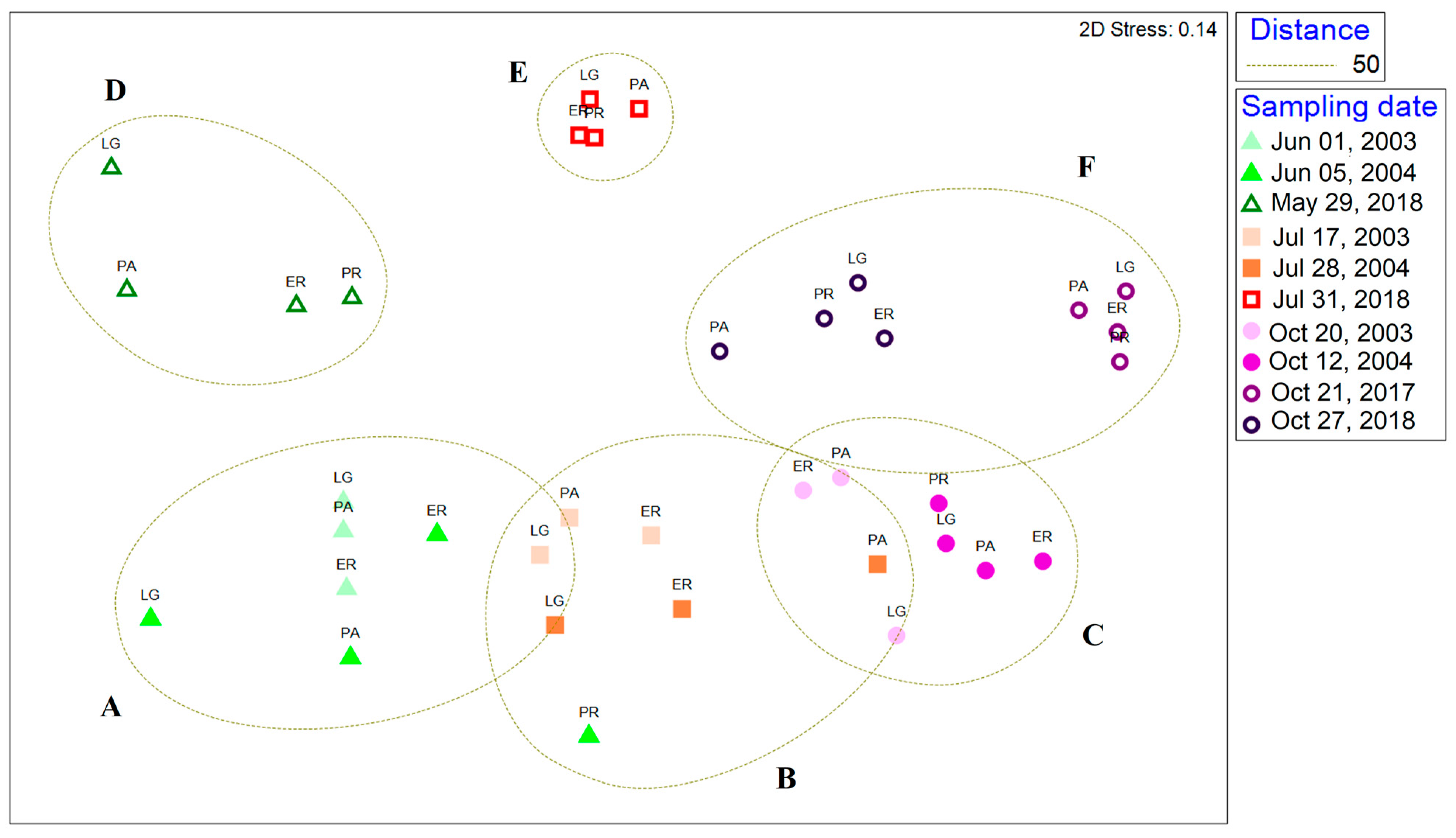
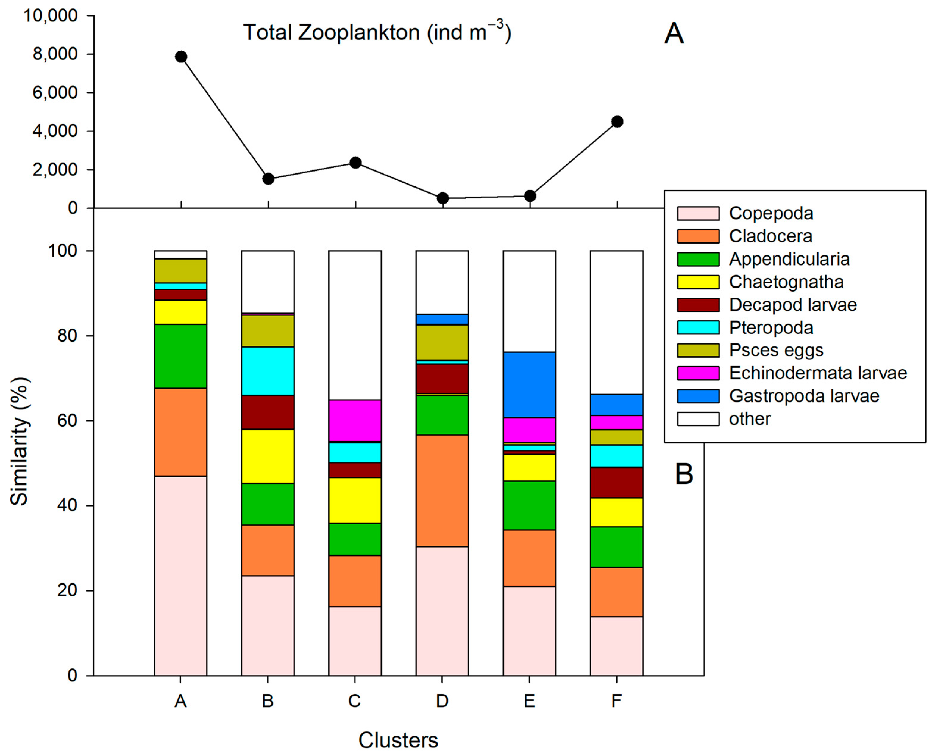
3.5. Comparison with Zooplankton from 2003 to 2004

The abundance of zooplankton groups fluctuates considerably over the months. Therefore, the comparison with previous data from 2003 to 2004 taken from Lavaniegos et al., 2012 [11] focused on the dates that most closely coincided with the period of 2018–2019 (Table 2), i.e., 29 May 2018, for the spring, 31 July 2018, for the summer, and, for the autumn, there were two sampling dates (October 2017 and 2018). It was not possible to compare the winters, either due to a lack of sampling (2003 and 2018) or because the sampling was carried out on very different dates, late winter in 2004 (7 March) and early winter in 2019 (4 January). Only stations ER, LG, PA, and PR were selected since they were the only ones sampled during 2003–2004.
Few zooplankton groups showed significant differences in the spring. Copepods were notably more abundant in spring 2003 and 2004, with medians of 5995 and 8796 ind m−3, respectively compared to 2018 (328 ind m−3). Chaetognaths were more abundant in 2004 compared to 2003 and 2018 (Table 2). The cladoceran Penilia avirostris was absent in spring 2004, and its abundance in 2003 was significantly lower than in 2018. Other groups such as polychaetes, barnacle larvae, and gastropod larvae were absent in the spring of both 2003 and 2004, as was the cladoceran Podon sp.
Interannual differences in copepod abundance were also observed in the summer, being higher in 2003 (median = 3781 ind m−3) than in 2004 (421 ind m−3) and 2008 (425 ind m−3). Appendicularians also showed a higher abundance in 2003 (Table 2). Decapod larvae and fish eggs and larvae were more abundant in 2003 and 2004 than in 2018. Again, in the summers of 2003 and 2004, polychaetes, gastropod larvae, and Podon sp. were absent. The other cladoceran species did not show interannual differences.
It was in the autumn when a greater number of zooplankton groups were found with significant differences (Table 2). The copepods presented the highest abundance in October 2017 and the lowest in October 2003 (medians of 4775 and 526 ind m−3, respectively). Other groups with the highest abundances in October 2017 were appendicularians, doliolids, siphonophores, and medusae, while P. tergestina was most abundant in October 2018 and echinoderm larvae were most abundant in October 2003. Polychaetes, heteropods, gastropod larvae, and Podon were only found in the autumns of 2017 and 2018.
The multivariate analysis revealed the formation of six clusters at a cutoff distance of 50 (Figure 10). Both the periods (2003–2004 and 2017–2018) and the seasons were kept separate in different clusters. Thus, the spring, summer, and autumn samples from 2003 to 2004 were grouped into clusters A, B, and C, while the corresponding 2017–2018 seasons were grouped into clusters D, E, and F. The overall ANOSIM test was significant (R = 0.912, p = 0.01). Pairwise comparisons were significant in most cases (p < 0.04), except for the comparison between clusters B and D (p = 0.05), B and E (p = 0.05), and that between clusters D and E (p = 0.29). This means that the main interannual differences occurred in the spring and autumn, but the summers were more similar. The dissimilarity between the spring clusters (A and D) was 40% and was mainly due to the abundance of copepods (Table 2). Regarding the autumn, the dissimilarity between clusters C and F was 35% and was mainly due to meroplanktonic components: gastropod larvae, decapod larvae, and fish eggs were very abundant in October 2017–2018 compared to 2003–2004, while the opposite was true for echinoderm larvae.
In all the clusters, the groups that contributed most to the internal similarity were copepods, followed by cladocerans (Figure 11). However, the proportion in which these two groups combined contributed was variable, with a maximum influence in the spring clusters (cluster A = 68%, cluster D = 57%), regardless of their real abundance (Table 2). In contrast, in the summer and fall clusters, their contribution was less than 40%. Appendicularians also contributed significantly to the similarity in clusters, but no seasonal trend was apparent. In contrast, chaetognaths showed the greatest influence on the similarity in the summer and autumn clusters, mainly during 2003–2004.

4. Discussion

Despite the biological diversity and economic importance of Bahía de Los Ángeles and its status as a biosphere reserve [32], little effort has been devoted to the study of zooplankton in this bay. More attention has been paid to benthic invertebrates [7,9,33,34,35,36,37,38] or fishes [39]. Furthermore, most of these studies had limited coverage to the southern part of the bay, and only the most recent ones have studied the northern part.
The first zooplankton study of BLA reported that the copepod abundance constituted 62% [10]. That study was conducted in the summer, whereas the present investigation indicated a month-to-month variation of 41 to 69%. Lavaniegos et al. [11] reported a wider range (34–98%) during the quarterly samplings conducted during 2003–2004. The relative abundance of copepods varies greatly depending on the amount of cladocerans and meroplankton, which show a marked seasonality. In absolute terms, the mean zooplankton density reported for the summer of 1999 was higher than in the summers of 2003–2004 and 2017–2018 (7800, 2198, and 2734 ind m−3, respectively), although these averages were associated with wide ranges of abundance: 660–38,100 ind m−3 [10], 253–4391 ind m−3 [11], and 311–13,333 ind m−3 (this study). It is evident that the high abundance obtained by Nelson and Eckert compared to the other studies is mainly due to the use of a net with a smaller mesh size (153 µm).
Nelson and Eckert [10] found less zooplankton abundance in the northern region of BLA than in the southern region, which is like what was observed in the present study. This was even though the northern region of BLA has been considered to have a high primary productivity [18]. There was probably an underestimation of the zooplankton abundance in the northern region, because it is deeper, and vertically migrating organisms could have been out of reach of the net, since the trawls were superficial and in the morning.

4.1. Structure of Zooplankton in the Context of Other Adjacent Coastal Regions

The little research on zooplankton is not limited to BLA but also to other coastal regions of the Mexican and Central American Pacific. Several studies describe zooplankton based on occasional sampling, but few analyze a complete annual cycle. According to the inventory carried out by De la Lanza-Espino et al. [40], there are around 52 coastal lagoons and estuaries in the Gulf of California, although Brusca et al. [41] raised that number to 208 sites. However, research on a complete seasonal cycle of zooplankton community is only found in a few studies. In the peninsular coast, there are studies of the seasonal variation in BLA and La Paz Bay, while, for the continental coast, there are for two lagoons (Las Guásimas and Navachiste) and four estuarine systems (El Verde, Urías, El Rey, and El Pozo). In these and other regions shown in Table 3, the zooplankton abundance was lower using a net with a larger mesh to collect the plankton. The zooplankton abundance reported for BLA was in the same order of that of other regions where a 200 µm mesh was used. In contrast, a larger mesh (300 to 500 µm) resulted in values one or two orders of magnitude lower due to the escape of small organisms.
The maximum abundance of zooplankton in the Gulf of California occurred during the spring in ecosystems located further north, while on the Nayarit and most of the Sinaloa coasts this occurred in the autumn. The latter could be due to the connection between the coastal ecosystem and the open sea, as in the El Verde estuary, where the sand bar was open from August to November, with an input of larval and postlarval shrimp and other marine elements [42]. In contrast, the Urias estuary was modified for port operations, maintaining permanent communication with the sea, increasing the abundance of holoplankton (Table 3). Another factor influencing the peak abundance in the Urías Estuary was the discharge of wastewater, producing a proliferation of the ctenophore Pleurobrachia bachei, which in turn preyed on copepods and ichthyoplankton [43]. The El Rey and El Pozo estuaries also maintain permanent communication with the open sea, but the anthropogenic influence is less than that of the Urias estuary [44]. On most of the gulf coasts, holoplankton consisted of copepods (>70%). In the meroplankton, decapod larvae (mainly crabs) and shrimp postlarvae were dominant. However, other organisms dominated in some locations, such as barnacle larvae in Nayarit estuaries, echinoderm larvae in BLA during 2003–2004 [11], and bivalve larvae during 2017–1018 (this study).
Table 3. Total zooplankton abundance and percentage of holoplankton in different coastal regions of the Gulf of California, West Coast of Baja California and USA, and Eastern Tropical Pacific. Dominant groups (DGs) of holoplankton and meroplanktonic larvae and date of maximum abundance (DMA) are shown. BC: Baja California, BCS: Baja California Sur.
RegionDateMeshAbundance (ind m−3)Holoplankton (%)Meroplank. Source
(µm)RangeMeanDMARangeMeanDGDG
GULF OF CALIFORNIA
Bahía de Los Ángeles, BC2003–2004200908–12,7034626Spring78–9994CopepodsEchinoderms.[11]
2017–2019200493–10,8303114May80–9891Coppods,
cladocerans
Bivalves,
decapods
This study
La Paz Bay, BCS1975–19762191.020–19,000 16.018May75–9991CopepodsGastropods[45]
1990–1992300163–3393948Spring82–9791CopepodsDecapods[46]
2003–2004333276–1651793June69–8475Copepods, cladoceransDecapods[47]
Ensenada Aripez (La Paz)1975–1976219950–4050 12583August78–9690CopepodsDecapods[45]
Las Guasimas Lagoon, Sonora201030057–1000 Spring 96CopepodsDecapods,
gastropods
[48]
Navachiste Lagoon, Sinaloa2002–2003505 Spring 67CopepodsDecapods[49]
El Verde Estuary, Sinaloa1977–19784501–189 237August–September0–5010CopepodsDecapods[42]
Urías Estuary, Sinaloa1976–1977450429–1007651November44–9275CtenohoresDecapods[43]
El Rey Estuary, Nayarit1972–1973200525–13,667 12977September CopepodsCirripedians[44]
El Pozo Estuary, Nayarit1972–1973200783–28,343 15808August CopepodsCirripedian,[44]
WESTERN COAST OF BAJA CALIFORNIA AND USA
Neah Bay, Washington1961110, 215174–19,869 35682June99–10099CopepodsEchinoderms, cirripedians[50]
Newport, Oregon1970240105–28,374 410,127June 96CopepodsBivalves[51]
Tomales Bay, California1978–197924032–965 5256February74–9995CopepodsDecapods[52]
Santa Monica Bay, California1976–1977253121–32,631 46040April98–10099CopepodsCirripedians[53]
Todos Santos Bay, BC1982–198350540–367194Summer80–9590CopepodsDecapods[54]
1986–19873001030–10,8404208Summer77–9890CopepodsBryozoans[55]
Vizcaino Bay, BC1997–2013505131–394260Spring–Summer95–9997CopepodsDecapods[56]
Gulf of Ulloa, BCS1998–2013505154–787408Summer73–9991CopepodsDecapods[56]
Magdalena Bay, BCS1997–2001333673–36,64514,229Summer68–9887CopepodsDecapods[57]
EASTERN TROPICAL PACIFIC
El Salado Estuary, Jalisco20015052–5234Winter 49ChaetognathsDecapods[58]
Chamela Bay, Jalisco2001–2002150173–3631 41512April20–9685CopepodsMollusks[59]
Navidad Bay, Jalisco2010–201125040–3600 1985November85–9791CopepodsDecapods[60]
Barra de Navidad Lagoon, Jalisco2009–201050537–441143Winter6–3320CopepodsDecapods[61]
Manzanillo Bay, Colima2001–2002150155–6777 42878April62–9891CopepodsMollusks[59]
Nuxco Lagoon, Guerrero1974?10,000–50,000 623,333May CopepodsCirripedians[62]
Coyuca Lagoon, Guerrero199925039–282109July77–10092CopepodsDecapods[63]
Chautengo Lagoon, Guerrero1974?500–10,000 63833May CopepodsCirripedians[62]
Chacahua Lagoon, Oaxaca1996–19975009–1054327June4–1912MedusaeDecapods, fishes[64]
La Pastoría Lagoon, Oaxaca1996–199750032–402258December7–6630Copepods, mysidsDecapods[64]
San Agustín Bay, Oaxaca1990–199125017–246103May83–9581CopepodsDecapods[65]
Santa Cruz Bay, Oaxaca1990–199125066–1685856May76–9773CopepodsEchinoderms, decapods[65]
Chahué Bay, Oaxaca1990–1991250128–750542May44–9464CopepodsGastropods[65]
Tangolunda Bay, Oaxaca1990–199125090–1126471May72–9482CopepodsDecapods[65]
Campon Lagoon, Chiapas19972502228–26452436May95–9796CopepodsCirripedians, gastropods[66]
Chantuto Lagoon, Chiapas1997250549–32331891July93–9996CopepodsCirripedians[66]
Teculapan Lagoon, Chiapas199725040–362201July64–8072CopepodsCirripedians[66]
Cerritos Lagoon, Chiapas1997250757–825791July89–9994CopepodsDecapods[66]
Panzacola Lagoon, Chiapas1997250235–448341May6–10053CopepodsCirripedians[66]
Jiquilisco Bay, El Salvador2009125408–1807 11125Summer13–9763CopepodsCirripedians, decapods[67]
2013–2014150 1028January 89CopepodsDecapods, gastropods[68]
Culebra Bay, Costa Rica2000500269–3625 11532February–March CopepodsDecapods[69]
Gulf of Dulce, Costa Rica1997–19981533456–22,030 49865April95–9998CopepodsGastropods[70]
Gulf of Nicoya, Costa Rica19972801457–91424404April 74CopepodsCrustaceans[71]
Gulf of Montijo, Panama2009–2010243300–4010 11318May 84CopepodsDecapods[72]
Jaramijo Bay, Ecuador20083351923–6435 54179April92–9593Copepods, cladoceransFish eggs[73]
Salado Estuary, Ecuador2016–201730027–1330380October6–7439CopepodsCirripedians[74]
1 Value inferred from graph; 2 average of surface and bottom tows (1–3 m) in one station; 3 5 m depth; 4 one station; 5 average from high and low tides in one station; 6 approximate abundance, since it was expressed in orders of magnitude, (?) not specified.
The seasonal variation in zooplankton in the coastal ecosystems of the western coast of Baja California has received attention in Todos Santos Bay [54,55], Magdalena Bay [57], Vizcaino Bay, and the Gulf of Ulloa [56]. Some studies carried out on the coasts of California, Oregon, and Washington are also presented in Table 3 to provide a reference for more temperate areas. In temperate environments, the peak abundance occurs mainly in the summer, and the highest values were also observed when plankton was collected using finer mesh nets [50,51,53,55,57]. The only exception was Tomales Bay, California, which had a low mean abundance (256 ind m−3) near the bay entrance, despite using a 240 µm mesh [52]. A later study [75] reported a higher geometric mean (3300 ind m−3) for zooplankton from this bay using the same mesh size. Unfortunately, this author does not present monthly values and so they were not included in Table 3. On the other hand, Castro-Longoria and Hamman [54] found a low abundance of zooplankton in Todos Santos Bay, which they attributed to the influence of the 1982–1983 El Niño event. This is difficult to argue for, lacking information on the typical conditions in the bay, and because they used a coarse mesh (505 µm). The locality with the highest abundance of zooplankton on the western coast of Baja California was Magdalena Bay, with an average of 14,229 ind m−3 combining values from the years 1997–1998 and 2000–2001, when extreme changes in the ENSO cycle occurred [57]. It was during the warm phase of ENSO (August 1997–April 1998) that there was a greater abundance, while in the cold phase (January 2000–March 2001), it decreased mainly due to the decrease in copepods. In Vizcaino Bay and the Gulf of Ulloa, which have a wide coastal platform and extensive communication with the oceanic zone, the zooplankton presented a greater proportion of tunicates (salps and doliolids) than in the coastal lagoons and small bays. Tunicates represented on average 16% of the total zooplankton in Vizcaino Bay and 7% in the Gulf of Ulloa [56], while it was only 1% in Todos Santos Bay [54,55] and 0.4% in Magdalena Bay [57]. However, the relative abundance may mask the real number of tunicates, since the percentages are low due to the large number of copepods present. Considering the absolute abundance, a range of 18–59 ind m−3 is observed for tunicates from the western coast of Baja California from the sites reported in Table 3, with the sole exception of Todos Santos Bay where they averaged 0.7 ind m−3 [54]. Regarding the Gulf of California, the abundance of tunicates was contrasting between the peninsular and continental coasts, being higher in the former (23–86 ind m−3) than in the latter (0–1 ind m−3).
In the Mexican tropical Pacific, there are studies that describe the seasonal variability in zooplankton for the coasts of all states from Jalisco to Chiapas except for Michoacán (Table 3). Considering the locations where the sampling was carried out with mesh nets ≤ 250 µm, the abundance showed a wide range (17–6777 ind m−3), but below that found in the coastal sites of the Gulf of California and the western coast of Baja California and the U.S.A. The monthly mean was estimated in the Mexican tropical Pacific to be below 400 ind m−3 for Coyuca Lagoon, Guerrero, San Agustín Bay, Oaxaca, and Teculapan and Panzacola Lagoons in Chiapas. The low abundance in these lagoons could be due to the different environmental factors. For example, in Coyuca Lagoon, the abundance and diversity of zooplankton increased in July, when communication with the sea is established. Furthermore, when the river discharge increases, it promotes saline stratification in the lagoon, causing a drastic decrease in marine species [63]. A low presence of marine species was also observed in the Teculapan and Panzacola lagoons, which are part of an estuarine system in southern Chiapas, and both are relatively far from the entrance that connects with the sea [66]. It is worth mentioning that in that study, the sampling was only carried out in two months, but they were included in Table 3, as they are considered representative months of contrasting seasons (dry and rainy). Regarding San Agustín Bay, the low abundance of zooplankton was attributed to the sampling time that occurred during the morning [65]. However, Tongolunda Bay was also sampled during daylight hours in the same study and a greater abundance was recorded. Evidently, the sampling was limited in time and space to be able to estimate the zooplankton abundance more accurately.
The most productive period on the tropical Pacific coast usually occurs in the spring or summer. It is important to note the effect that stratification has on these coastal lagoons. Franco-Gordo et al. [60] showed that the abundance of zooplankton in Navidad Bay, Jalisco, as well as the seasonal succession of taxonomic groups is driven by periods of stratification and mixing induced by upwelling. The lowest abundance of zooplankton is recorded during the summer when the water column is stratified. The percentage of holoplankton was high in Navidad Bay (91%), which contrasts with the 20% reported for the small lagoon Barra de Navidad, located inside the bay [61]. While the loss of small copepods through the mesh used to sample the lagoon (500 µm) may be the reason for a low percentage of holoplankton, the disproportionate amount of decapod larvae found is related to the variety of benthic biotopes that make the Barra de Navidad lagoon a crab nursery [76].
Most tropical coastal environments showed a dominance of copepods as in the temperate zone, but there were some exceptions. For example, in Chacahua Lagoon, Oaxaca, jellyfish dominated, while in La Pastoría Lagoon, a codominance of copepods and mysids was observed, even though both lagoons are part of the same lagoon system [64]. Both lagoons have an inlet that communicates with the sea, but they suffer from silting problems and require dredging for their rehabilitation [77]. The data reported in Table 3 come from a sampling carried out when Chacahua Lagoon was closed, and this explains the scarcity of copepods and other groups. In contrast, La Pastoría had communication with the sea and a greater diversity of zooplankton groups was observed. However, in both lagoons, meroplankton was very abundant and was dominated by decapod larvae, but Chacahua fish larvae were also abundant.
The seasonal dynamics on the coasts of Central America and Ecuador is very similar to that observed in the Mexican tropical Pacific. Information was found for Jiquilisco Bay in El Salvador, and several locations in Costa Rica, Panama, and Ecuador (Table 3). Among the particularities of these systems, a high abundance can be mentioned in the Gulf of Dulce, Costa Rica [70]. That is a very complete study where three depths were sampled, although Table 3 only refers to surface trawls at a station close to the mouth of the gulf. An inverse relationship was found between the quantity of zooplankton and dissolved oxygen, the concentration of which decreases towards the interior of the gulf. Vertically, the greatest abundance of zooplankton was concentrated in the surface layer due to the presence of a strong oxycline [70]. In all the environments of Central America, a dominance of copepods and high percentages of holoplankton (63–98%) were found. In Ecuador, holoplankton represented 93%, and a codominance of copepods and cladocerans was observed in Jaramijó Bay [73], while in the Salado Estuary there was a greater quantity of meroplankton with a dominance of barnacle larvae [74].
According to Ambler et al. [78], the seasonal variation in zooplankton in estuarine systems may be due to the changes in temperature, photoperiod, and river discharges and may also reflect the changes in the coastal hydrology, such as upwellings. In the different subtropical and tropical coastal lagoons discussed above, evidence of all these effects was found. Upwelling events have a significant influence on the bays of the western coast of Baja California and the tropical Pacific [56,60]. In the most protected ecosystems, such as lagoons and estuaries, the saline stratification during the rainy season is decisive and sometimes causes the collapse of marine species [63]. Some studies in which the sampling was carried out during an annual cycle were not included in Table 3, because they presented the abundance and composition data in aggregate form, and it was not possible to elucidate all the details of the seasonal variability. That was the case in the analysis of the zooplankton composition from the Huave lagoon system in Oaxaca [79] and the Utría Estuary in Colombia [80]. In both systems, a greater abundance was reported during the dry season, while in the Manta and Pedernales Bays in Ecuador, the wet season was the richest in zooplankton [81,82].

4.2. Abundance and Seasonality of Cladocerans

Cladocerans were found to be one of the crustacean groups with the greatest seasonality in BLA, due to their life cycle. During the cold and less productive season, they disappear from the water column, producing diapausing eggs, which sink into the sediment waiting for better environmental conditions to hatch and restart the parthenogenic phase of their reproductive cycle [83]. The abundance of cladocerans found in the present investigation differs from that in previous studies carried out in BLA [10,11]. It is only possible to compare summer–autumn averages, since this was the time of year that Nelson and Eckert [10] sampled and presented the information in aggregate form. They estimated 2% of cladocerans with respect to the total zooplankton during 1999, while Lavaniegos et al. [11] found 4% for summer–autumn of 2003 and 34% in 2004. Finally, in the present study, cladocerans were 16% for summer–autumn of 2017 and 42% in 2018. As can be observed, there is great interannual variability in the proportion of these crustaceans. Hernández-Nava and Álvarez-Borrego [12] found low percentages (0.3–7%), but they sampled during September–December of 2009 exclusively in the El Rincón area. The seasonality of cladocerans has been documented in many coastal studies (Table 4), where cladocerans virtually disappear from the water column in the winter.
In the present study, the highest abundance of Penilia avirostris occurred in autumn 2017, but in 2018 they were more abundant in the spring. In other regions of the Gulf of California and around the world, the peak abundance of cladocerans occurs more frequently in the spring or summer (23 and 48% of the cases reported in Table 4, respectively). The occurrence of a peak in abundance during the autumn was observed at two sites in the Gulf of California (BLA and Estero Urias, Sinaloa), as well as in the Zuari Estuary, India, in the Mediterranean (Istanbul coast), and two sites from the Atlantic Ocean (Vigo coast and Mondego Estuary, Brazil). All of them except the Zuari Estuary are subtropical or temperate ecosystems. Only two sites recorded maximum abundances of P. avirostris in the winter (Tolo Harbor, Hong Kong, and the Estuary of Rio Escuro, Brazil). It should be noted that in sites where there is information for two or more years, the peak in abundance does not always recur in the same season of the year. For example, in BLA, the maximum abundance occurred in May 2018 and not during the autumn as during 2003–2004 [11], and in the Escuro River Estuary, the peaks occurred in July 2004 and March 2005, which correspond to the austral winter and summer, respectively [107].
Piontkovski et al. [89] compared the seasonal dynamics of P. avirostris in subtropical regions (coast of Vigo, Gulf of Trieste, and Gulf of Sevastopol) located between 43 and 46° N with that of the Gulf of Oman (23.5° N), concluding that in tropical areas, this species is present all year round, while in temperate areas, it is limited to the summer. However, as mentioned above, there were subtropical regions with high abundance in the autumn, some far enough north to be considered temperate. Regarding the disappearance of this species during one season of the year, most studies show that it can disappear in the winter even in tropical regions such as the bays of Oaxaca [65], or in coastal lagoons during the rainy season [66]. In other sites, such as Santa Elena Bay [84], Tolo Harbor, and the Zhujang River Estuary [88], although it was present throughout the year, it showed a drastic decrease during December–January. Regarding the abundance of P. avirostris, even excluding the values derived from the 450 and 500 µm mesh, the maximum abundance varied greatly between the regions (Table 4). The lowest values (1–100 ind m−3) were recorded more in the tropical than in the subtropical zone (eight and two sites, respectively). However, the high-density peaks (10,000–50,000 ind m−3) corresponded equally to the ecosystems in the subtropical and tropical zones.
The second most abundant cladoceran in BLA was Pseudoevadne tergestina. This species had a less extensive distribution than P. avirostris, being absent from some temperate sites such as Santa Monica Bay and the Mondego Estuary (Table 4). Instead, other cladoceran species such as Evadne nordmanni and Pleopis (=Podon) polyphemoides were found [53,100]. The maximum abundance of P. tergestina was in the range of 10–1000 ind m−3 in most temperate sites and half of the tropical ones (Table 4), which is an order of magnitude lower than that of P. avirostris. This is partly explained by the fact that P. tergestina is a more carnivorous organism than P. avirostris. In fact, the morphological differences in feeding structures, among others, determine that cladocerans are no longer considered a taxonomic entity and were fragmented into several orders [109]. Thus, Penilia avirostris and Pseudoevadne tergestina now belong to two different orders (Ctenopoda and Onycophoda). Regarding the phenology of P. tergestina, most studies agree that the peak in abundance occurs during the spring or summer. There is a tendency for these peaks in abundance to occur during the spring in tropical latitudes and in the summer for subtropical–temperate latitudes (Table 4).
Freshwater species were also found in some estuaries. For example, in the Paraíba do Sul River Estuary, Brazil, a gradient was observed in the distribution of marine and freshwater species, with P. avirostris being more abundant in the external stations and Moina micrura in the internal ones where the salinity decreases dramatically with the rainfall [104]. In the Mondego Estuary, the abundance of the freshwater cladoceran Daphnia longispina increases during winter–spring, while the marine species Pleopis polyphemoides and Evadne nordmanni do so in summer–autumn [100]. The intrusion of freshwater species into lagoons and estuaries obviously depends on the volume of incoming freshwater, but also on the coastal geomorphology. For example, the Estero El Verde, Sinaloa, has an elongated shape and a narrow mouth communicating with the sea. During the rainy season, the flooding of the El Quelite River brings a large volume of water to the estuary, and then only the freshwater cladocerans Moina wierzejskii and M. micrura are observed [42].

5. Conclusions

Bahia de Los Ángeles behaves like a temperate ecosystem and shows seasonality in the abundance of various groups, mainly in the proportion of copepods, cladocerans, and meroplankton. The comparison with other temperate and tropical coastal lagoons in the eastern Pacific showed a dominance of copepods, mainly those less sheltered and not influenced by a freshwater input. In contrast, sheltered regions, have a high abundance of meroplankton as shrimp or crab larvae.
The dominant cladoceran species was Penilia avirostris, as in other coastal ecosystems around the world. Given the high seasonal and interannual variability in these organisms, the abundance estimates in BLA and other tropical ecosystems in Mexico and Central America can only be tentative, due to the sampling with time gaps. It is required to intensify the study of zooplankton in the coastal ecosystems of Mexico, in which the seasonal dynamics of the species that inhabit the water column are still unknown. Mexico has a great diversity of biotopes, but they are fragile, and changes in zooplankton can be a good indicator of the health of the ecosystem.

Supplementary Materials

The following supporting information can be downloaded at: https://www.mdpi.com/article/10.3390/d17050316/s1, Table S1: Data base of zooplankton abundance by sampling station from Bahía de Los Ángeles during 2017–2019.

Author Contributions

Conceptualization, B.E.L. and G.O.-M.; methodology, B.E.L.; software, B.E.L.; validation, B.E.L., G.O.-M. and J.L.C.-R.; formal analysis, B.E.L. and G.O.-M.; investigation, B.E.L., G.O.-M. and J.L.C.-R.; resources, B.E.L.; data curation, B.E.L. and G.O.-M.; writing—original draft preparation, B.E.L.; writing—review and editing, B.E.L., G.O.-M. and J.L.C.-R.; visualization, B.E.L.; supervision, B.E.L.; project administration, B.E.L.; funding acquisition, B.E.L. All authors have read and agreed to the published version of the manuscript.

Funding

This research was funded by Ensenada Center for Scientific Research and Higher Education (CICESE), through the project “Zooplankton variability as a function of climate changes at different scales” (625114).

Institutional Review Board Statement

Not applicable.

Data Availability Statement

The original contributions presented in this study are included in the article/Supplementary Materials. Further inquiries can be directed to the corresponding author.

Acknowledgments

We would like to thank Eduardo Guillén Diaz and Victor Moreno Rivera for their support during the sampling. Elena Solana Arellano provided logistical support.

Conflicts of Interest

The authors declare no conflicts of interest.

Abbreviations

The following abbreviations are used in this manuscript:
BLABahía de Los Ángeles
GCGulf of California
ETPEastern Tropical Pacific
OSTIASea Surface Temperature and Sea Ice Analysis
SSTSea Surface Temperature
ERStation El Rincon
PRStation Punta Roja
CEStation Central
BLStation Bahía de Los Ángeles city
PAStation Punta Arena
LGStation La Gringa
CIStation Cerraja Island

References

  1. McLean, J.H. Marine mollusks from Los Angeles Bay, Gulf of California. Trans. San Diego Soc. Nat. Hist. 1961, 12, 449–476. [Google Scholar]
  2. Townsend, C.H. Voyage of the ‘Albatross’ to the Gulf of California in 1911. Bull. Am. Mus. Nat. Hist. 1916, 35, 399–476. [Google Scholar]
  3. Brinton, E.; Fleminger, A.H.; Siegel-Causey, D. The temperate and tropical planktonic biotas of the Gulf of California. Cal. Coop. Ocean. Fish. 1986, 27, 228–266. [Google Scholar]
  4. Lindsay, G.E.; Engstrand, I.H.W. History of scientific exploration in the Sea of Cortes. In Island Biogeography of the Sea of Cortes; Case, T.J., Cody, M.L., Ezcurra, E., Eds.; Oxford University Press: New York, NY, USA, 2002; pp. 3–13. [Google Scholar]
  5. Danemann, G.D.; Ezcurra, E.; Velarde, E. Conservación ecológica. In Bahía de Los Ángeles: Recursos Naturales y Comunidad; Danemann, G.D., Ezcurra, E., Eds.; Pronatura Noroeste, Secretaría de Medio Ambiente y Recursos Naturales, Instituto Nacional de Ecología, San Diego Natural History Museum: México, D.F., Mexico, 2008; pp. 695–729. [Google Scholar]
  6. Barnard, J.L.; Grady, J.R. A biological survey of Bahia de Los Angeles, Gulf of California. Mexico I. General account. Trans. San Diego Soc. Nat. Hist. 1968, 15, 51–66. [Google Scholar]
  7. Coan, E.V. A biological survey of Bahia de Los Angeles, Gulf of California, Mexico. III. Benthic Mollusca. Trans. San Diego Soc. Nat. Hist. 1968, 15, 107–132. [Google Scholar]
  8. Reish, D.J. A biological survey of Bahia de Los Angeles, Gulf of California, Mexico. II. Benthic polychaetous annelids. Trans. San Diego Soc. Nat. Hist. 1968, 15, 67–106. [Google Scholar]
  9. Barnard, J.L. A biological survey of Bahia de Los Angeles, Gulf of California, Mexico. IV. Benthic Amphipoda (Crustacea). Trans. San Diego Soc. Nat. Hist. 1969, 15, 175–228. [Google Scholar]
  10. Nelson, J.D.; Eckert, S.A. Foraging ecology of whale sharks (Rhincodon typus) within Bahía de Los Angeles, Baja California Norte, México. Fish. Res. 2007, 84, 47–64. [Google Scholar] [CrossRef]
  11. Lavaniegos, B.E.; Heckel, G.; Ladrón de Guevara, P. Seasonal variability of copepods and cladocerans in Bahía de Los Ángeles (Gulf of California) and importance of Acartia clausi as food for whale sharks. Cienc. Mar. 2012, 38, 11–30. [Google Scholar] [CrossRef]
  12. Hernández-Nava, M.F.; Álvarez-Borrego, S. Zooplankton in a whale shark (Rhincodon typus) feeding area of Bahía de Los Angeles (Gulf of California). Hidrobiológica 2013, 23, 198–208. [Google Scholar]
  13. Villagómez-Vélez, S.I.; Carreón-Palau, L.; Mejía-Zepeda, R.; González-Armas, R.; Aguíñiga-García, S.; Vázquez-Haikin, A.; Galván-Magaña, F. Fatty acid composition of whale shark (Rhincodon typus), and zooplankton in two aggregation sites in the Gulf of California. Reg. Stud. Mar. Sci. 2024, 76, 103577. [Google Scholar] [CrossRef]
  14. Amador-Buenrostro, A.; Serrano-Guzmán, S.J.; Argote-Espinoza, M.L. Numerical model of the circulation induced by the wind at Bahia de Los Angeles, BC., Mexico. Cienc. Mar. 1991, 17, 39–57. [Google Scholar] [CrossRef]
  15. Cavazos, T. Clima. In Bahía de Los Ángeles: Recursos Naturales y Comunidad; Danemann, G.D., Ezcurra, E., Eds.; Pronatura Noroeste, Secretaría de Medio Ambiente y Recursos Naturales, Instituto Nacional de Ecología, San Diego Natural History Museum: México, D.F., Mexico, 2008; pp. 67–90. [Google Scholar]
  16. Álvarez-Borrego, S. Oceanografía. In Bahía de Los Ángeles: Recursos Naturales y Comunidad; Danemann, G.D., Ezcurra, E., Eds.; Pronatura Noroeste, Secretaría de Medio Ambiente y Recursos Naturales, Instituto Nacional de Ecología, San Diego Natural History Museum: México, D.F., Mexico, 2008; pp. 45–65. [Google Scholar]
  17. Marinone, S.G.; Lavín, M.F. Residual flow and mixing in the large islands regions of the central Gulf of California. In Nonlinear Processes in Geophysical Fluid Dynamics; Velasco-Fuentes, O.U., Sheinbaum, J., Ochoa-de la Torre, J.L., Eds.; Kluwer Academic Publishers: Amsterdam, The Netherlands, 2003; pp. 213–236. [Google Scholar]
  18. Delgadillo-Hinojosa, F.; Gaxiola-Castro, G.; Segovia-Zavala, J.A.; Muñoz-Barbosa, A.; Orozco-Borbón, M.V. The effect of vertical mixing on primary production in a bay of the Gulf of California. Estuar. Coast. Shelf Sci. 1997, 45, 135–148. [Google Scholar] [CrossRef]
  19. Byrne, J.V.; Emery, K.O. Sediments of the Gulf of California. Bull. Geol. Soc. Am. 1960, 71, 983–1010. [Google Scholar] [CrossRef]
  20. Millán-Núñez, E. Red tide in Bahia de Los Angeles. Cienc. Mar. 1988, 14, 51–55. [Google Scholar] [CrossRef]
  21. Gilmartin, M.; Revelante, N. The phytoplankton characteristics of the barrier island lagoons of the Gulf of California. Estuar. Coast. Mar. Sci. 1978, 7, 29–47. [Google Scholar] [CrossRef]
  22. Canino-Herrera, S.R.; Gaxiola-Castro, G.; Segovia-Zavala, J.A. Effect of physical processes on the variation of chlorophyll, seston and primary productivity in the northern inlet of Bahia de Los Angeles (Summer 1986). Cienc. Mar. 1990, 16, 67–85. [Google Scholar] [CrossRef]
  23. Muñoz-Barbosa, A.; Gaxiola-Castro, G.; Segovia-Zavala, J.A. Temporal variability of primary productmty, chlorophyll and seston in Bahia de Los Angeles, Gulf of California. Cienc. Mar. 1991, 17, 47–68. [Google Scholar] [CrossRef]
  24. Parker, R.H. Zoogeography and ecology of some macroinvertebrates, particularly mollusks, in the Gulf of California and the continental slope off Mexico. Vidensk. Meddr. Dan. Naturn. Foren. 1964, 126, 1–178. [Google Scholar]
  25. Halfar, J.; Strasser, M.; Riegl, B.; Godinez-Orta, L. Oceanography, sedimentology and acoustic mapping of a bryomol carbonate factory in the northern Gulf of California, Mexico. In Cool-Water Carbonates: Depositional Systems and Palaeoenvironmental Controls; Geological Society, London, Special Publications: Bath, UK, 2006; No. 255; pp. 197–215. [Google Scholar]
  26. Yamaji, I. Illustrations of The Marine Plankton of Japan; Hoikusha Publ. Co.: Osaka, Japan, 1979; 537p. [Google Scholar]
  27. Todd, C.D.; Laverack, M.S. Coastal Marine Zooplankton: A Practical Manual for Students; Cambridge University Press: Cambridge, UK, 1991; pp. 1–106. [Google Scholar]
  28. Young, C.M.; Sewell, M.A.; Rice, M.E. (Eds.) Atlas of Marine Invertebrate Larvae; Academic Press: San Diego, CA, USA, 2002; 626p. [Google Scholar]
  29. Onbè, T. Ctenopoda and Onychopoda (=Cladocera). In South Atlantic Zooplankton; Boltovskoy, D., Ed.; Backhuys Publishers: Leiden, The Netherlands, 1999; pp. 797–814. [Google Scholar]
  30. Donlon, C.J.; Martin, M.; Stark, J.; Roberts-Jones, J.; Fiedler, E.; Wimmer, W. The operational sea surface temperature and sea ice analysis (OSTIA) system. Remote Sens. Environ. 2012, 116, 140–158. [Google Scholar] [CrossRef]
  31. Clarke, K.R.; Gorley, R.N.; Somerfield, P.J. Change in Marine Communities: An Approach to Statistical Analysis, 3rd ed.; PRIMER-E: Plymouth, UK, 2014; 262p. [Google Scholar]
  32. SEMARNAT (Secretaría de Medio ambiente y Recursos Naturales). Decreto Por el que se Declara Área Natural Protegida, Con la Categoría de Reserva de la Biosfera, la Zona Marina Conocida Como Bahía de los Ángeles, Canales de Ballenas y de Salsipuedes; Diario Oficial de la Federación: Mexico, D.F., Mexico, 2007; 14p. [Google Scholar]
  33. Donath-Hernández, F.E. Cumaceos de Bahía de Los Ángeles, Baja California, Mexico (Crustacea, Peracarida). Cienc. Mar. 1993, 19, 461–471. [Google Scholar] [CrossRef]
  34. Leija-Tristán, A. Tamaño y densidad de Neaxius vivesi (Thalassinoidea: Axiidae), en Bahía de Los Ángeles, Baja California, México. Rev. Biol. Trop. 1994, 42, 719–721. [Google Scholar]
  35. Del Moral-Flores, L.F.; González-Acosta, A.F.; Espinosa-Pérez, H.; Ruiz-Campos, G.; Castro-Aguirre, J.L. Lista anotada de la ictiofauna de las islas del golfo de California, con comentarios sobre sus afinidades zoogeográficas. Rev. Mex. Biodivers. 2013, 84, 184–214. [Google Scholar] [CrossRef]
  36. Glockner Fagetti, A.; Calderon-Aguilera, L.; Herrero-Perezrul, M.D. Density decrease in an exploited population of brown sea cucumber Isostichopus fuscus in a Biosphere Reserve from the Baja California peninsula, Mexico. Ocean Coast Manag. 2016, 121, 49–59. [Google Scholar] [CrossRef]
  37. Herrero-Pérezrul, M.D.; Reyes-Bonilla, G.; Granja-Fernández, R. Effects of environmental factors on the abundances of the basket stars Astrocaneum spinosum and Astrodictyum panamense (Ophiuroidea: Gorgonocephalidae) in the northern Gulf of California, Mexico. Mar. Biol. Res. 2017, 13, 210–219. [Google Scholar]
  38. Alvarado-Rodríguez, J.F.; Nava, H.; Cabral-Tena, R.A.; Norzagaray-López, C.O.; Calderón-Aguilera, L.E. Contribución de los heterótrofos a la calcificación secundaria en arrecifes marginales del Pacífico mexicano. Hidrobiológica 2023, 33, 169–178. [Google Scholar]
  39. Viesca-Lobatón, C.; Balart, E.F.; González-Cabello, A.; Mascareñas-Osorio, I.; Aburto-Oropeza, O.; Reyes-Bonilla, H.; Torreblanca, E. Peces arrecifales. In Bahía de los Ángeles: Recursos Naturales y Comunidad; Danemann, G.D., Ezcurra, E., Eds.; Pronatura Noroeste, Secretaría de Medio Ambiente y Recursos Naturales, Instituto Nacional de Ecología, San Diego Natural History Museum: Mexico, D.F., Mexico, 2008; pp. 385–427. [Google Scholar]
  40. De la Lanza-Espino, G.; García-Calderón, J.L.; Tovilla-Hernández, C.; Arredondo-Figueroa, J.L. Ambientes y Pesquerías en el Litoral Pacífico Mexicano; Instituto Nacional de Estadística, Geografía e Informática: Aguascalientes, México, 1993; 97p. [Google Scholar]
  41. Brusca, R.C.; Cudney-Bueno, R.; Moreno-Báez, M. Gulf of California Esteros and Estuaries: Analysis, State of Knowledge and Conservation Priority Recommendations. Final Report to the David and Lucile Packard Foundation by the Arizona-Sonora Desert Museum. 2006. Available online: https://www.rickbrusca.com/http___www.rickbrusca.com_index.html/Papers_files/Packard%20Final%20Report%20SMALL.pdf (accessed on 8 April 2020).
  42. Sánchez-Osuna, L. Variaciones Estacionales del Zooplancton en el Estero El Verde, Sinaloa, México, con Especial Referencia a los Copepoda Calanoidea y Cladocera. Bachelor’s Thesis, National Polytechnic Institute, Mexico City, Mexico, 1980. [Google Scholar]
  43. Álvarez-León, R. Hidrología y zooplancton de tres esteros adyacentes a Mazatlán, Sinaloa, México. An. Cent. Cienc. Mar Limnol. UNAM 1980, 7, 177–194. [Google Scholar]
  44. Cortés-Guzmán, A.S.; Martínez-Guerrero, A. Identificación y cuantificación de larvas pedivelígeras de Crassostrea corteziensis Hertlein y balánidos, en el plancton de dos estuarios de San Blas, Nayarit, Pacífico de México. An. Cent. Cienc. Mar Limnol. UNAM 1979, 6, 37–51. [Google Scholar]
  45. Signoret, M.; Santoyo, H. Aspectos ecológicos del plancton de la Bahía de La Paz, Baja California sur. An. Inst. Cienc. Mar Limnol UNAM 1980, 7, 217–248. [Google Scholar]
  46. Lavaniegos, B.E.; González-Navarro, E. Grupos principales del zooplancton durante El Niño 1992–93 en el Canal de San Lorenzo, Golfo de California. Rev. Biol. Trop. 1999, 47 (Suppl. S1), 129–140. [Google Scholar]
  47. Hernández-Trujillo, S.; Nava-Torales, A.; Esqueda-Escárcega, G.M. El cambio estacional del mesozooplancton en la Bahía de La Paz, Baja California Sur, México (2003–2004). In Proceedings of the XX Congreso Nacional de Ciencia y Tecnología del Mar, Cabo San Lucas, Mexico, 1–4 October 2013; Secretaría de Educación Media Superior: Toluca de Lerdo, Mexico, 2013. [Google Scholar]
  48. Álvarez-Tello, F.J.; López-Martínez, J.; Funes-Rodríguez, R.; Lluch-Cota, D.B.; Rodríguez-Romero, J.; Flores-Coto, C. Composición, estructura y diversidad del mesozooplancton en Las Guásimas, Sonora, un sitio Ramsar en el Golfo de California, durante 2010. Hidrobiologica 2015, 25, 401–410. [Google Scholar]
  49. De Silva-Dávila, R.; Palomares-García, R.; Zavala-Norzagaray, A.; Escobedo-Urías, D.C. Ciclo anual de los grupos dominantes del zooplancton en Navachiste, Sinaloa. In Contributions to the Study of East Pacific Crustaceans; Hendrickx, M.E., Ed.; Instituto de Ciencias del Mar y Limnología, Universidad Nacional Autónoma de México: Mexico City, Mexico, 2006; Volume 4, pp. 26–39. [Google Scholar]
  50. Peterson, W.K.; Anderson, G.C. Net zooplankton data from the northeast Pacific Ocean: Columbia River efluent area, 1961, 1962. Department of Oceanography, University of Wahington. Tech. Rep. 1966, 160, 1–225. [Google Scholar]
  51. Peterson, W.T.; Miller, C.B. Year to year variations in the planktology of the Oregon upwelling zone. Fish. Bull. 1975, 73, 642–653. [Google Scholar]
  52. Johnston, D.J. The Zooplankton Communities of Tomales Bay, California. Master’s Thesis, University of the Pacific, Stockton, CA, USA, 1980. [Google Scholar]
  53. Soule, D.F.; Oguri, M. Marine studies of San Pedro Bay, California. Part 13, The Marine ecology of Marina del Rey Harbor, California; Allan Hancock Foundation Technical Series No. 2; Allan Hancock Foundation (Harbors Environmental Projects) and the Office of Sea Grant Programs (University of Southern California): Los Angeles, CA, USA, 1977; pp. 1–424. [Google Scholar]
  54. Castro-Longoria, E.; Hammann, M.G. Zooplankton biomass and community structure in Todos Santos Bay, B.C., Mexico, during the 1982-83 El Niño event. Cienc. Mar. 1989, 15, 1–20. [Google Scholar] [CrossRef]
  55. Jiménez-Pérez, L.C. Temporal variation of zooplankton in Todos Santos Bay, Baja California, Mexico. Cienc. Mar. 1989, 15, 81–96. [Google Scholar] [CrossRef]
  56. Lavaniegos, B.E.; Molina-González, O.; Murcia-Riaño, M. Zooplankton functional groups from the California Current and climate variability during 1997–2013. Oceánides 2015, 30, 45–62. [Google Scholar] [CrossRef]
  57. Hernández-Trujillo, S.; Esqueda-Escárcega, G.; Palomares-García, R. Variabilidad de la abundancia de zooplancton en Bahía Magdalena, Baja California Sur, México (1997–2001). Lat. Am. J. Aquat. Res. 2010, 38, 438–446. [Google Scholar] [CrossRef]
  58. Navarro-Rodríguez, M.C.; Flores-Vargas, R.; González-Guevara, L.F. Variación estacional de los principales grupos zooplanctónicos del área natural protegida estero El Salado, Jalisco, México. Rev. Bio Cienc. 2015, 3, 103–115. [Google Scholar]
  59. Briseño-Avena, C. Biomasa y Composición del Zooplancton en la Bahía de Chamela, Jalisco y la Bahía de Manzanillo, Colima Durante un Ciclo Anual (2001–2002). Bachelor’s Thesis, University of Guadalajara, Jalisco, Mexico, 2004. [Google Scholar]
  60. Franco-Gordo, C.; Ambriz-Arreola, I.; Kozak, E.R.; Gómez-Gutiérrez, J.; Plascencia-Palomera, V.; Godínez-Domínguez, E.; Hinojosa-Larios, A. Seasonal succession of zooplankton taxonomic group assemblages in surface waters of Bahia de Navidad, Mexico (November 2010–December 2011). Hidrobiologica 2015, 25, 335–345. [Google Scholar]
  61. Flores-Vargas, R.; Navarro-Rodríguez, M.C.; González-Guevara, L.F.; Saucedo-Lozano, M. Variación estacional de los principales grupos zooplanctónicos y parámetros físicos del área natural protegida Laguna Barra de Navidad, Jalisco. Acta Pesq. 2017, 3, 34–50. [Google Scholar]
  62. Martínez-Guerrero, A. Distribución y variación estacional del zooplancton en cinco lagunas costeras del estado de Guerrero. México. An. Cent. Cienc. Mar Limnol UNAM 1978, 5, 201–214. [Google Scholar]
  63. Álvarez-Silva, C.; Torres-Alvarado, M.R. Composición y abundancia del zooplancton de la Laguna de Coyuca, Guerrero, México. Hidrobiologica 2013, 23, 241–249. [Google Scholar]
  64. Pantaleón-López, B.; Aceves, G.; Castellanos, I.A. Distribución y abundancia del zooplancton del complejo lagunar Chacahua-La Pastoría, Oaxaca, México. Rev. Mex. Biodivers. 2005, 76, 63–70. [Google Scholar]
  65. Sosa-Rosas, L. Composición y Variación del Zooplancton Presente en Algunas Localidades del Desarrollo Turístico Bahías de Huatulco, Oaxaca, Durante 1990–1991. Master’s Thesis, National Autonomous University of Mexico, Mexico City, Mexico, 1995. [Google Scholar]
  66. Álvarez-Silva, C.; Miranda-Arce, G.; De Lara-Isassi, G.; Gómez-Aguirre, S. Zooplancton de los sistemas estuarinos de Chantuto y Panzacola, Chiapas, en época de secas y de lluvias. Hidrobiologica 2006, 16, 175–182. [Google Scholar]
  67. Cuellar, T.C. Composición y abundancia del zooplancton. In El Ecosistema de Manglar de la Bahía de Jiquilisco; Rivera, C.G., Cuellar, T.C., Eds.; University of El Salvador: San Salvador, El Salvador, 2010; pp. 83–100. [Google Scholar]
  68. Galdámez-Castaneda, K.M. Composición y Abundancia del Zooplancton en el Área Los Remos, Bahía de Jiquilisco, El Salvador. Bachelor’s Thesis, University of El Salvador, San Salvador, El Salvador, 2014. [Google Scholar]
  69. Bednarski, M.; Morales-Ramírez, A. Composition, abundance and distribution of macrozooplankton in Culebra Bay, Gulf of Papagayo, Pacific coast of Costa Rica and its value as bioindicator of pollution. Rev. Biol. Trop. 2004, 52, 105–119. [Google Scholar]
  70. Quesada-Alpízar, M.A. Caracterización, Composición, Abundancia y Biomasa del Zooplancton en el Golfo Dulce Durante el Período 1997–1998. Master’s Thesis, University of Costa Rica, San Jose, Costa Rica, 2001. [Google Scholar]
  71. Brugnoli-Olivera, E.; Díaz-Ferguson, E.; Delfino-Machin, M.; Morales-Ramírez, A.; Dominici-Arosemena, A. Composition of the zooplankton community, with emphasis in copepods, in Punta Morales, Golfo de Nicoya, Costa Rica. Rev. Biol. Trop. 2004, 52, 897–902. [Google Scholar]
  72. Grimaldo, M.; Chang, J.; Muñoz, E.; Averza, A. Abundancia estacional del zooplancton en el Golfo de Montijo, Pacifico panameño. Tecnociencia 2013, 15, 33–42. [Google Scholar]
  73. Gualancañay, E.; Tapia, M.E.; Naranjo, C.; Cruz, M.; Villamar, F. Caracterización biológica de la Bahía de Jaramijó en la costa ecuatoriana, 2008. Acta Oceanogr. Pac. 2010, 16, 33–52. [Google Scholar]
  74. Castro-Madrid, R.A. Distribución y Abundancia del Zooplancton en un Área del Estero Salado, Entre Puente El Velero y Puente Zig-Zag, de la Ciudad de Guayaquil. Bachelor’s Thesis, University of Guayaquil, Guayaquil, Ecuador, 2017. [Google Scholar]
  75. Kimmerer, W.J. Distribution patterns of zooplankton in Tomales Bay, California. Estuaries 1993, 16, 264–272. [Google Scholar] [CrossRef]
  76. Álvarez-del Castillo, M.; Hendrickx, M.E.; Rodríguez, S. Crustáceos decápodos de la Laguna Barra de Navidad, Jalisco, México. Proc. San Diego Soc. Nat. Hist. 1992, 27, 1–9. [Google Scholar]
  77. González, G.; Rodríguez, E.A. El sistema lagunar: Cambios naturales, antropogénicos y su impacto en el ecosistema estuarino. In Chacahua: Reflejos de un Parque. Comisión Nacional de Áreas Naturales Protegidas; Alfaro, M., Sánchez, G., Eds.; Comisión Nacional de Áreas Protegidas, Programa de las Naciones Unidas para el Desarrollo, Secretaría de Medio ambiente y Recursos Naturales; Editorial Plaza y Valdés: México, D.F., Mexico, 2002; pp. 39–58. [Google Scholar]
  78. Ambler, J.W.; Cloern, J.E.; Hutchinson, A. Seasonal cycles of zooplankton from San Francisco Bay. Hydrobiologia 1985, 129, 177–197. [Google Scholar] [CrossRef]
  79. López-Serrano, A.; Serrano-Guzmán, S.J. Composición por grupos y abundancia del mesozooplancton en la Laguna Inferior (Sistema Lagunar Huave, Oaxaca, México), en mayo y septiembre-octubre de 2007. Cienc. Y Mar 2013, 19, 3–14. [Google Scholar]
  80. Valencia, B.; Giraldo, A.; Rivera-Gómez, M.; Izquierdo, V.; Cuellar-Chacón, A. Effects of seasonal upwelling on hydrography and mesozooplankton communities in a Pacific tropical cove off Colombia. Rev. Biol. Trop. 2019, 67, 945–962. [Google Scholar] [CrossRef]
  81. Naranjo, C.; Tapia, M. Variabilidad estacional del plancton en la Bahía de Manta en la costa ecuatoriana, durante el 2011. Acta Oceanogr. Pacif. 2013, 18, 65–74. [Google Scholar]
  82. Naranjo, C.; Tapia, M. Productividad planctónica en la Bahía de Pedernales, Manabí-Ecuador durante el 2013. Acta Oceanogr. Pacif. 2014, 19, 31–42. [Google Scholar]
  83. Egloff, D.A.; Fofonoff, P.W.; Onbé, T. Reproductive biology of marine cladocerans. Adv. Mar. Biol. 1997, 31, 79–167. [Google Scholar]
  84. Mejillón-del Pezo, Y.E. Estudio Sobre la Composición, Abundancia y Variación Espacio-Temporal del Orden Cladocera, Presentes en la Bahía de Santa Elena-La Libertad, Durante Octubre 2004 a Octubre 2005. Bachelor’s Thesis, Statal University of Santa Elena, La Libertad Canton, Ecuador, 2008. [Google Scholar]
  85. Jang, M.C.; Shin, K.; Jang, P.G.; Lee, W.J.; Choi, K.H. Mesozooplankton community in a seasonally hypoxic and highly eutrophic bay. Mar. Freshw. Res. 2015, 66, 719–729. [Google Scholar] [CrossRef]
  86. Hwang, O.M.; Shin, K.; Baek, S.H.; Lee, W.J.; Kim, S.; Jang, M.C. Annual variations in community structure of mesozooplankton by short-term sampling in Jangmok Harbor of Jinhae Bay. Ocean Polar Res. 2011, 33, 235–253. [Google Scholar] [CrossRef]
  87. Onbé, T. Seasonal fluctuations in the abundance of populations of marine cladocerans and their resting eggs in the inland Sea of Japan. Mar. Biol. 1985, 87, 83–88. [Google Scholar] [CrossRef]
  88. Tang, K.; Chen, Q.C.; Wong, C.K. Distribution and biology of marine cladocerans in the coastal waters of southern China. Hydrobiologia 1995, 307, 99–107. [Google Scholar] [CrossRef]
  89. Piontkovski, S.A.; Fonda-Umani, S.; De Olazabal, A.; Gubanova, A.D. Penilia avirostris: Regional and global patterns of seasonal cycles. Int. J. Ocean. Oceanogr. 2012, 6, 9–25. [Google Scholar]
  90. Goswami, S.C.; Devassy, V.P. Seasonal fluctuations in the occurrence of Cladocera in the Mandovi-Zuari estuarine waters of Goa. Indian J. Mar. Sci. 1991, 20, 138–142. [Google Scholar]
  91. Ezhilarasan, P.; Kanuri, V.V.; Sivasankar, R.; Kumar, P.S.; Murthy, M.R.; Rao, V.R.; Ramu, K. Surface mesozooplankton assemblages in a tropical coastal upwelling ecosystem: Southeastern Arabian Sea. Cont. Shelf Res. 2018, 168, 28–38. [Google Scholar] [CrossRef]
  92. Atienza, D.; Saiz, E.; Skovgaard, A.; Trepat, I.; Calbet, A. Life history and population dynamics of the marine cladoceran Penilia avirostris (Branchiopoda: Cladocera) in the Catalan Sea (NW Mediterranean). J. Plankton Res. 2008, 30, 345–357. [Google Scholar] [CrossRef]
  93. Calbet, A.; Garrido, S.; Saiz, E.; Alcaraz, M.; Duarte, C.M. Annual zooplankton succession in coastal NW Mediterranean waters: The importance of the smaller size fractions. J. Plankton Res. 2001, 23, 319–331. [Google Scholar] [CrossRef]
  94. Pestoric, B.; Lučić, D.; Joksimović, D. Cladocerans spatial and temporal distribution in the coastal south Adriatic waters (Montenegro). Stud. Mar. 2011, 25, 101–120. [Google Scholar]
  95. Gülsahin, N.; Tarkan, A.N. Seasonal changes in distribution and abundance of the cladoceran species in relation to environmental factors in Gökova Bay (Mugla, Aegean Sea, Turkey). Fresen. Environ. Bull. 2012, 21, 1853–1863. [Google Scholar]
  96. Terbıyık-Kurt, T.; Polat, S. Seasonal distribution of coastal mesozooplankton community in relation to the environmental factors in Iskenderun Bay (Northeast Levantine, Mediterranean Sea). J. Mar. Biol. Assoc. UK 2013, 93, 1163–1174. [Google Scholar] [CrossRef]
  97. Isinibilir, M. Annual crustacean zooplankton succession (Copepoda and Cladocera) in the upper layer of Ahirkapi coastal waters (northeastern Sea of Marmara). Crustaceana 2009, 82, 669–678. [Google Scholar] [CrossRef]
  98. Johns, D.G.; Edwards, M.; Greve, W.; Sjohn, A.W.G. Increasing prevalence of the marine cladoceran Penilia avirostris (Dana, 1852) in the North Sea. Helgol. Mar. Res. 2005, 59, 214–218. [Google Scholar] [CrossRef]
  99. D’Elbée, J.; Lalanne, Y.; Castège, I.; Bru, N.; D’Amico, F. Response of planktonic cladocerans (Class: Branchiopoda) to short-term changes in environmental variables in the surface waters of the Bay of Biscay. Deep Sea Res. II 2014, 106, 87–98. [Google Scholar] [CrossRef]
  100. Primo, A.L.; Azeiteiro, U.M.; Marques, S.C.; Martinho, F.; Pardal, M.A. Changes in zooplankton diversity and distribution pattern under varying precipitation regimes in a southern temperate estuary. Estuar. Coast. Shelf Sci. 2009, 82, 341–347. [Google Scholar] [CrossRef]
  101. Oghenekaro, E.U.; Chigbu, P. Population dynamics and life history of marine Cladocera in the Maryland coastal bays, U.S.A. J. Coast. Res. 2019, 35, 1225–1236. [Google Scholar] [CrossRef]
  102. Ambler, J.W.; Kumar, A.; Moisan, T.A.; Aulenbach, D.L.; Day, M.C.; Dix, S.A.; Winsor, M.A. Seasonal and spatial patterns of Penilia avirostris and three tunicate species in the southern Mid-Atlantic Bight. Cont. Shelf Res. 2013, 69, 141–154. [Google Scholar] [CrossRef]
  103. Rose, K.; Roff, J.C.; Hopcroft, R.R. Production of Penilia avirostris in Kingston Harbour, Jamaica. J. Plankton Res. 2004, 26, 605–615. [Google Scholar] [CrossRef]
  104. Sterza, J.M.; Fernandes, L.L. Distribution and abundance of Cladocera (Branchiopoda) in the Paraíba do Sul river estuary, Rio de Janeiro, Brazil. Braz. J. Oceanogr. 2006, 54, 193–204. [Google Scholar] [CrossRef]
  105. Marazzo, A.; Valentin, J.L. Spatial and temporal variations of Penilia avirostris and Evadne tergestina (Crustacea, Branchiopoda) in a tropical bay, Brazil. Hydrobiologia 2001, 445, 133–139. [Google Scholar] [CrossRef]
  106. Miyashita, L.K.; Pompeu, M.; Gaeta, S.A.; Lopes, R.M. Seasonal contrasts in abundance and reproductive parameters of Penilia avirostris (Cladocera, Ctenopoda) in a coastal subtropical area. Mar. Biol. 2010, 157, 2511–2519. [Google Scholar] [CrossRef]
  107. Della Posta, P.; Leme, M.H.A. Variação temporal de cladóceros marinhos em uma região estuarina de Ubatuba, SP, Brasil. Bol. Inst. Pesca 2015, 41, 327–334. [Google Scholar]
  108. Viñas, M.D.; Ramírez, F.C.; Santos, B.A.; Marrari, M. Spatial and temporal distribution patterns of Cladocera in the Argentine Sea. Hydrobiologia 2007, 594, 59–68. [Google Scholar] [CrossRef]
  109. Fryer, G. Morphology and the classification of the so-called Cladocera. Hydrobiologia 1987, 145, 19–28. [Google Scholar] [CrossRef]
Figure 1. Map of Bahia de Los Ángeles and its location on the peninsular coast of the Gulf of California. The inset shows the bathymetry (m) and the sampling stations: BL = Bahia de Los Ángeles city, CE = central, CI = Cerraja Island, ER = El Rincón, LG = La Gringa, PA = Punta Arena, PR = Punta Roja. Topographic chart from GEBCO (https://download.gebco.net/, accessed on 17 March 2025).
Diversity 17 00316 g001
Figure 2. Sea surface temperature (SST) in Bahia de Los Ángeles during 2017–2018: (a) measured at each sampling station, (b) mean (±standard deviation) SST in situ and from satellite data (OSTIA). Station abbreviations are explained in the legend to Figure 1.
Diversity 17 00316 g002
Figure 3. Abundance per cubic meter of copepods, cladocerans, and nauplii in sampled stations (left). Their relative abundance in relation to total zooplankton is shown to the (right). (nd = no data).
Diversity 17 00316 g003
Figure 4. Abundance per cubic meter of appendicularians, chaetognaths, and pteropods in sampled stations (left). The relative abundance of these and other holoplankton groups is shown to the (right). (nd = no data).
Diversity 17 00316 g004
Figure 5. Larval abundance per cubic meter of decapods, bivalves, and gastropods in sampled stations (left). The relative abundance of these and other meroloplankton groups is shown to the (right). (nd = no data).
Diversity 17 00316 g005
Figure 6. Abundance per cubic meter of cladoceran species in sampled stations (left). Their relative abundance is shown to the (right). (nd = no data).
Diversity 17 00316 g006
Figure 7. Clustering of sampling stations based on abundances of zooplankton major taxa. Clusters formed at a cutoff distance of 65 (dashed line) are indicated in gray and numbered from 1 to 7. Symbols indicate the sampling date.
Diversity 17 00316 g007
Figure 8. Nonmetric multidimensional scaling ordination of sampling stations. Ellipses indicate the clusters formed in Figure 7. The size of symbols is scaled according to SST values.
Diversity 17 00316 g008
Figure 9. Characteristics of the clusters in median zooplankton abundance (A) and the contribution of the main taxa to the similarity (B). The selected taxa are a combination of the three with the greatest contribution to similarity in each group.
Diversity 17 00316 g009
Figure 10. Non-metric multidimensional scaling ordination of selected sampling stations from spring, summer, and autumn of 2003–2004 and 2017–2018. Ellipses indicate clusters formed at a distance of 50, identified by letters. Labels above symbols are abbreviated station names.
Diversity 17 00316 g010
Figure 11. Characteristics of the clusters in median zooplankton abundance (A) and the contribution of the main taxa to the similarity (B). The selected taxa are a combination of the four with the greatest contribution to similarity in each group.
Diversity 17 00316 g011
Table 1. Zooplankton groups from Bahía de Los Ángeles during 2017–2018. HP: holoplankton, MP: meroplankton, B: benthos.
Taxa/GroupHabitatFrequence
(Num. Samples)
Phylum ForaminiferaHP34
Phylum Cnidaria
   Subphylum Medusozoa
   HydromedusaHP46
   SiphonophoraHP32
   LarvaeMP10
Phylum CtenophoraHP5
Phylum ChaetognathaHP68
Phylum Annelida
   Polychaeta (pelagic)HP72
   Polychaeta (larvae)MP23
   Sipuncula (pelagosphera larva)MP18
Phylum Nemertea (pilidium larva)MP19
Phylum Mollusca
   PteropodaHP67
   Pterotracheoidea 1HP25
   Gastropoda (larvae)MP75
   Bivalvia (larvae)MP80
Phylum PlatyhelminthesB24
Phylum Brachiopoda (larvae)MP1
Phylum Phoronida (actinotroch larvae)MP24
Phylum Bryozoa (cyphonaute larvae)MP60
Phylum NematodaB4
Phylum Arthropoda
   Subphylum Crustacea
   CladoceraHP69
   OstracodaHP5
   Cirripedia (larvae)MP78
   Copepoda (adults and copepodites)HP81
   Copepoda (nauplii)HP13
   IsopodaB24
   CumaceaB1
   AmphipodaHP20
   Mysida 2HP5
   EuphausiaceaHP41
   Decapoda (mainly larvae)HP + MP75
   Stomatopoda (larvae)MP19
Phylum Echinodermata (larvae)MP41
Phylum Hemichordata (tornaria larvae)MP3
Phylum Chordata
   Subphylum CephalochordataB2
   Subphylum Tunicata
   AppendiculariaHP79
   DoliolidaHP28
   SalpidaHP17
   Subphylum Vertebrata
   Fishes (eggs)MP65
   Fishes (larvae)MP47
Invertebrates (larvae) 3MP37
1 Previously named Heteropoda; 2 close to the seabed; 3 mainly trochophores.
Table 2. Median abundance (ind m−3) of zooplankton groups from Bahía de Los Ángeles by season during 2017–2018 and 2003–2004. Only taxa with significant differences (α ≤ 0.05) for the Kruskal–Wallis test (H) are shown.
Season/Taxa2003200420172018Hp
Spring1 June
(n = 3)
5 June
(n = 3)
--29 May
(n = 4)
Fonaminifera00 26.50.039
Chaetognatha125 <17.40.025
Polychaeta00 <19.60.008
Copepoda59958796 3287.10.029
Gastropod larvae00 16.40.041
Cirripedia larvae00 39.40.009
Penilia avirostris00 178.60.014
Podon sp.00 99.40.009
Summer17 July
(n = 3)
28 July
(n = 3)
--31 July
(n = 4)
Polichaeta00 28.30.016
Pteropoda2864 18.20.016
Copepoda3781421 4256.00.050
Euphausiacea30 06.50.039
Appendicularia18312 287.40.025
Polychaeta larvae<11 07.50.024
Gastropoda larvae00 1238.30.016
Cirripedia larvae10 36.80.033
Decapoda larvae811 16.60.038
Echinodermata larvae0<1 57.20.028
Fish larvae814 <17.00.029
Fish eggs155 17.00.030
Autumn20 October
(n = 3)
12 October
(n = 4)
21 October
(n = 4)
27 October
(n = 4)
Hydromedusa6102537.80.050
Siphonophora314175113.20.004
Polychaeta0010315.20.007
Pterotracheoidea004210.50.015
Copepoda52616194775102211.70.008
Appendicularia242544515010.70.014
Ddoliolida2390274910.20.017
Polychaeta larvae516818.60.035
Gastropoda larvae00781013.40.004
Cirripedia larvae2010710.40.016
Echinodermata larvae150941968.40.038
Fish eggs<1051512.10.007
Pseudoevadne tergestina1354037910.60.014
Podon sp.00151313.40.004
Table 4. Mean abundance of two cladoceran species in different coastal regions during the high season.
Penilia avirostrisPseudoevadne tergestina
RegionMesh
(µm)
Abundance
(ind m−3)
DateAbundance
(ind m−3)
DateSource
EASTERN PACIFIC
Santa Monica Bay, California253460 2September 1976 [53]
Todos Santos Bay, BC50581 July 1983 [54]
Bahia de Los Ángeles, BC20051 October 2003538June 2003[11]
930 October 2004372July 2004[11]
1315October 2017 This study
1664May 20183027June 2018This study
La Paz Bay, BCS2191558 3May 1975235 3March 1976[45]
Urías Estuary, Sinaloa 1450152November 1976 [43]
San Agustín Bay, Oaxaca 125021 4May 19917 4May 1991[65]
Santa Cruz Bay, Oaxaca 125017 4May 199113 4May 1991[65]
Chahué Bay, Oaxaca 12506 4May 199179 4May 1991[65]
Tangolunda Bay, Oaxaca 125077 4May 199162 4May 1991[65]
Campon Lagoon, Chiapas25011May 1997 [66]
Santa Elena Bay, Ecuador33517,547 5 August 2005488 5March 2005[84]
WESTERN PACIFIC
Masan Bay, South Korea2002300July–August 2004–20051170July–August 2004–2005[85]
Jinhae Bay, South Korea20021,354 3June 200939,906 3August 2009[86]
Seto Inland Sea, Japan1007200 3July 19754600 3August 1975[87]
Zhujiang River Estuary, China12535 6August 19804 6June 1981[88]
Shanwei coast, China125500 6September 19827 6September 1982[88]
Tolo Harbor, Hong Kong1254500 6March 19911100May 1990[88]
INDIAN OCEAN
Gulf of Oman15050,000 7August 2004–2008 [89]
Mandovi Estuary, India330505 3May 1980368 3May 1980[90]
Estuario Zuari, India3304 3October 1980280 3December 1979[90]
Kochi coast, India20044August 2015754August 2015[91]
MEDITERRANEAN
Port Olimpic, Balearic Sea532500 3July-August 2003 [92]
Blanes Bay, Balearic Sea535650 6August 1995 [93]
Gulf of Trieste, Mediterranean1508770 7July 2004–2008 [89]
Montenegro coast, Adriatic Sea12529,900September 2009751August 2009[94]
Gulf of Gokova, Aegean Sea2002316September 200794July 2007[95]
Gulf of Alexandretta, Levantine Sea2001725April 200824July 2008[96]
Istanbul coast, Sea of Marmara1573317 3October 20052219 3April 2006[97]
Gulf of Sevastopol, Black Sea15015,000August 2004–2008 [89]
ATLANTIC OCEAN
Heligoland Bight, North Sea5003176July 2004 [98]
Bayona coast, Cantabrian Sea200600September 2001–2008600September 2001–2008[99]
Vigo coast, Cantabrian Sea1508 7November 2004–2006 [89]
Mondego Estuary, Portugal3352297November 2006 [100]
Maryland coast, USA200 38July 2012[101]
Virginia coast, USA80313July 2005–2007 [102]
Kingston Harbour, Jamaica20022,500 6July 19932000 6June 1992[103]
Paraiba do Sul River Estuary, Brazil7017,394 3March 2003 [104]
Guanabara Bay, Brazil200975March 19851204November 1985[105]
Ubatuba Bay, Brazil2005881 3June 2008 [106]
Rio Escuro Estuary, Brazil150905July 2004350July 2004[107]
1088March 2005 [107]
Mar del Plata, Argentina673200 3March 200025 3January 2001[108]
1 Reported as Penilia sp. and Evadne sp., 2 average of two stations external to Marina del Rey, 3 one station, 4 average of surface and 5 m tows, 5 average of diurnal and evening tows in one station, 6 value inferred from graph, 7 median.
Disclaimer/Publisher’s Note: The statements, opinions and data contained in all publications are solely those of the individual author(s) and contributor(s) and not of MDPI and/or the editor(s). MDPI and/or the editor(s) disclaim responsibility for any injury to people or property resulting from any ideas, methods, instructions or products referred to in the content.

