
Performance Analysis of Resonantly Driven Piezoelectric Sensors Operating in Amplitude Mode and Phase Mode

Abstract
:1. Introduction
2. Sensor
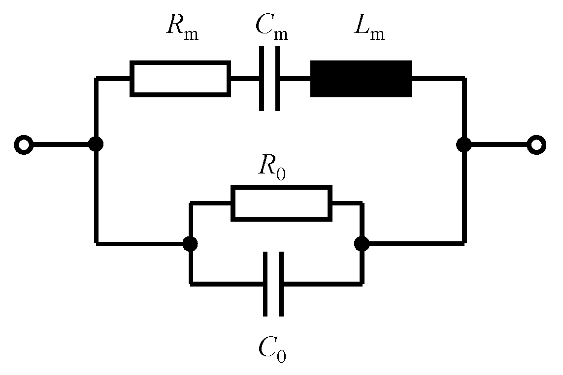
2.1. Electromechanical Resonator
2.2. Sensor Admittance
2.3. Exemplary Sensor
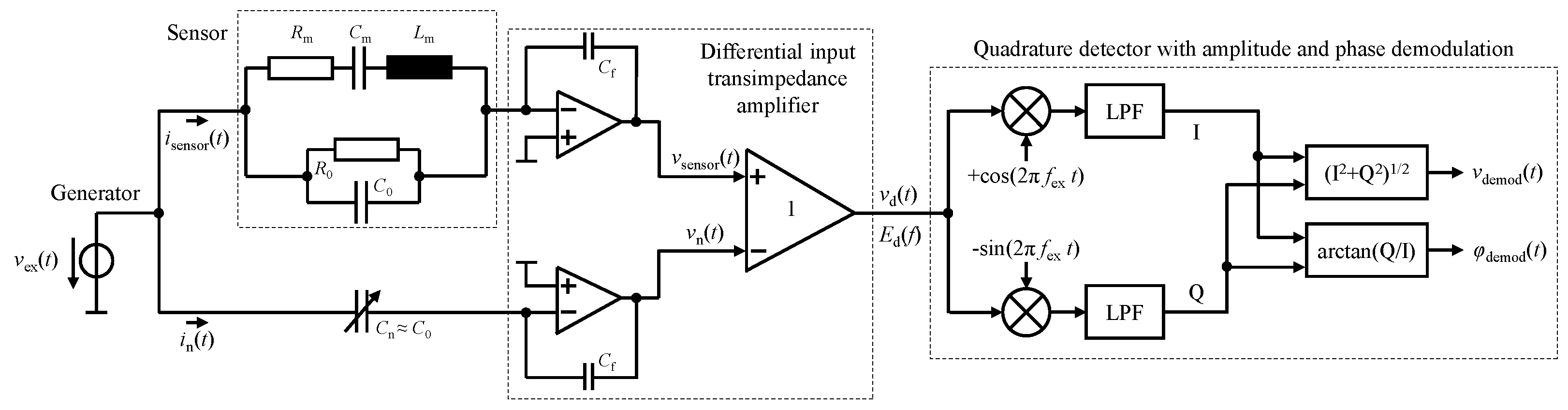
3. Sensor System
4. Sensitivity
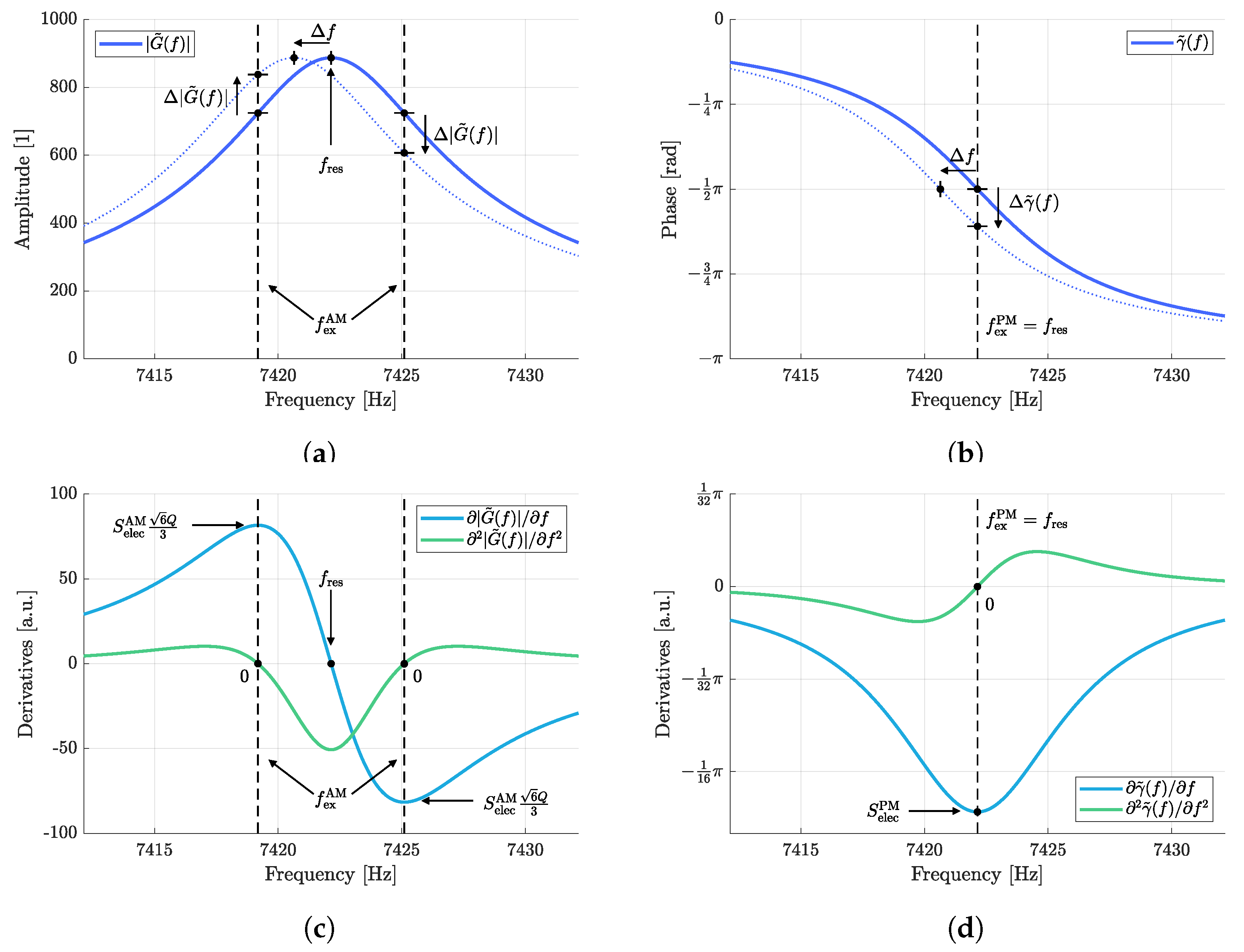
4.1. Functional Sensitivity
4.2. Electrical Sensitivity
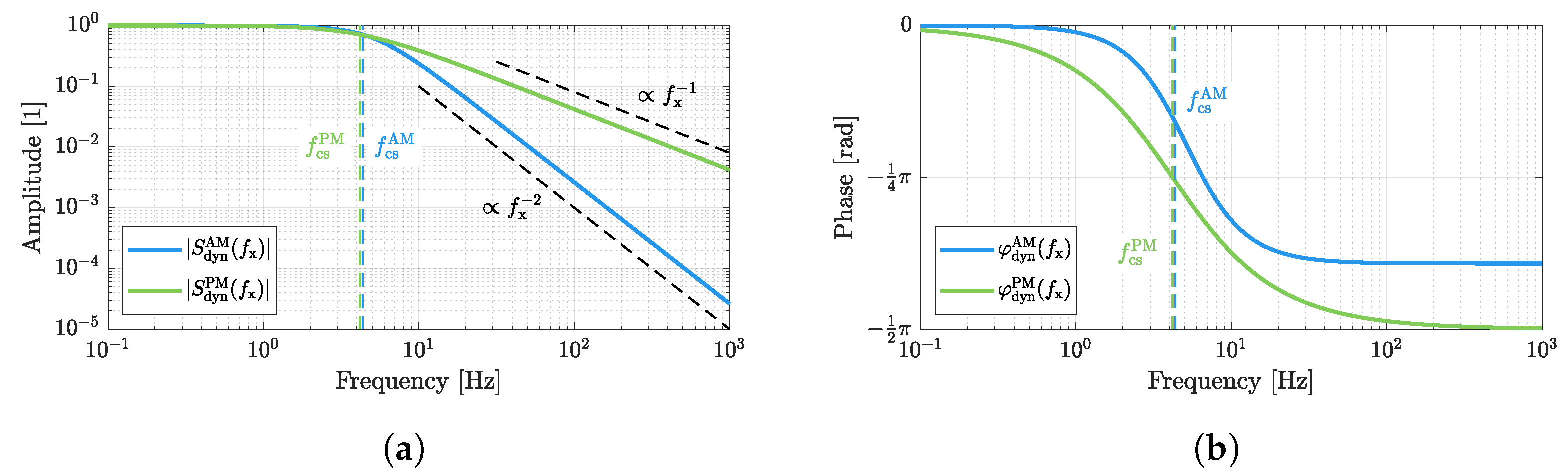
4.3. Dynamic Sensitivity
4.4. Overall Sensitivity
5. Noise
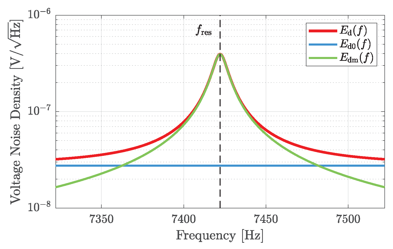
5.1. Voltage Noise
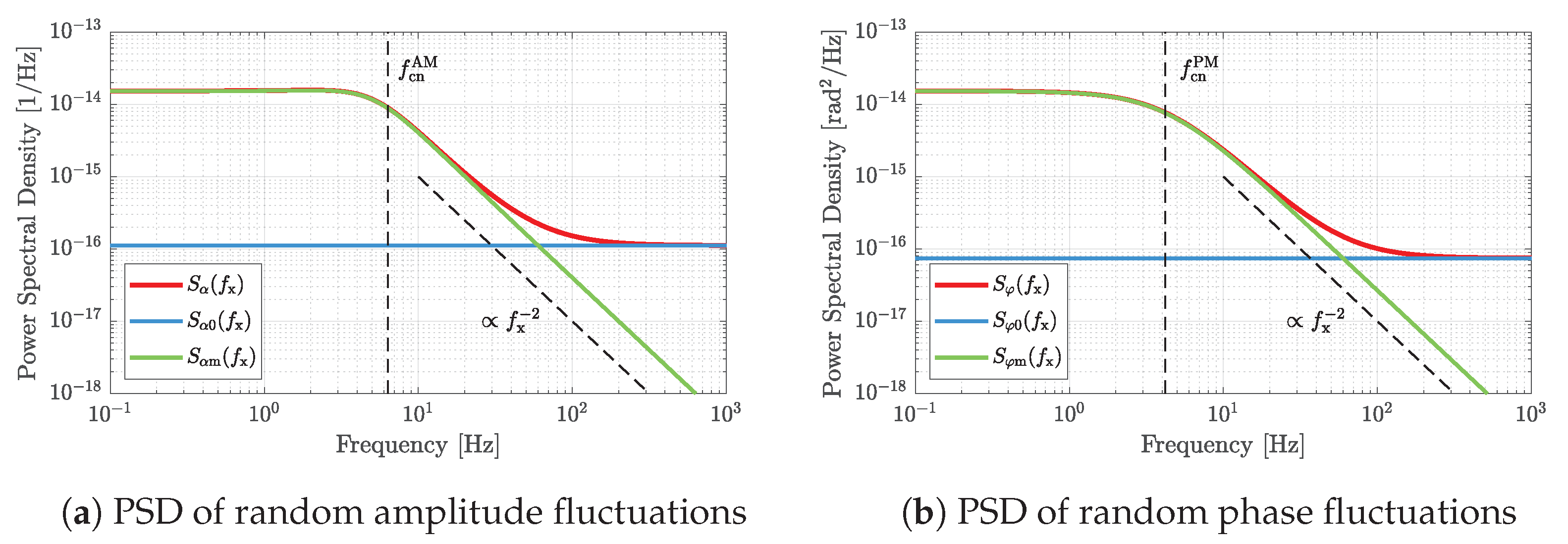
5.2. Amplitude Noise and Phase Noise
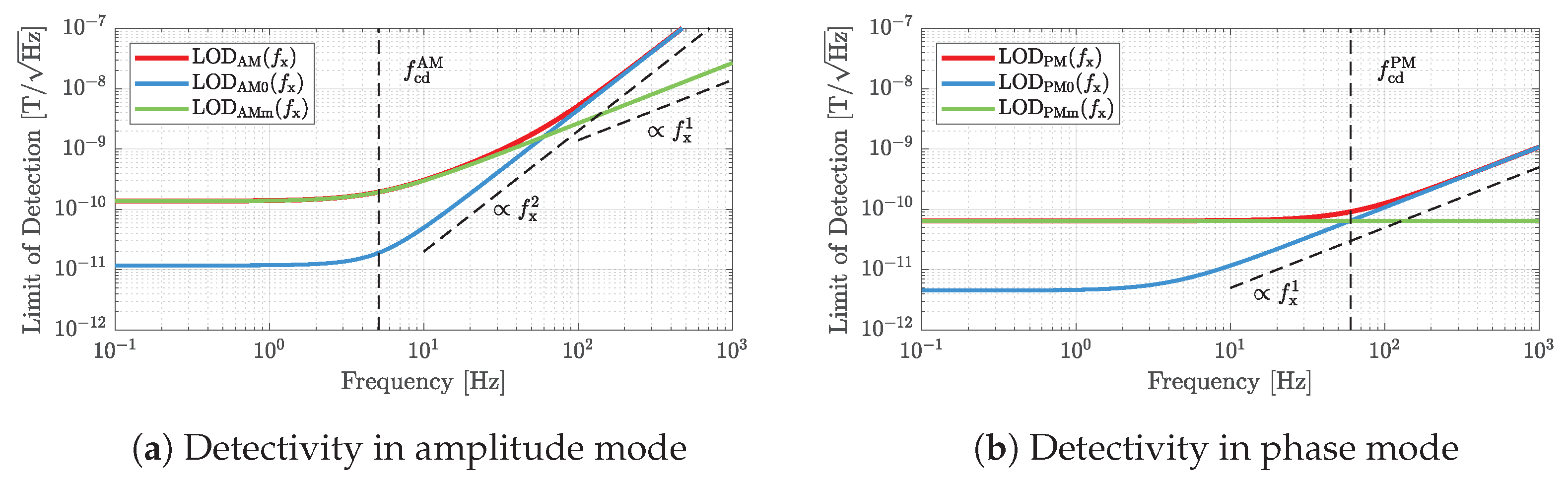
6. Detectivity
7. Conclusions
Author Contributions
Funding
Institutional Review Board Statement
Informed Consent Statement
Data Availability Statement
Conflicts of Interest
References
- Lang, H.P.; Gerber, C. Microcantilever Sensors. In Topics in Current Chemistry; Springer: Berlin/Heidelberg, Germany, 2008; Volume 285, pp. 1–27. [Google Scholar] [CrossRef]
- du Trémolet de Lacheisserie, E.; Peuzin, J. Magnetostriction and internal stresses in thin films: The cantilever method revisited. J. Magn. Magn. Mater. 1994, 136, 189–196. [Google Scholar] [CrossRef]
- Chen, G.Y.; Thundat, T.; Wachter, E.A.; Warmack, R.J. Adsorption-induced surface stress and its effects on resonance frequency of microcantilevers. J. Appl. Phys. 1995, 77, 3618–3622. [Google Scholar] [CrossRef]
- Barnes, J.R.; Stephenson, R.J.; Welland, M.E.; Gerber, C.; Gimzewski, J.K. Photothermal spectroscopy with femtojoule sensitivity using a micromechanical device. Nature 1994, 372, 79–81. [Google Scholar] [CrossRef]
- Ziegler, C. Cantilever-based biosensors. Anal. Bioanal. Chem. 2004, 379, 946–959. [Google Scholar] [CrossRef] [PubMed]
- Lee, J.H.; Hwang, K.S.; Park, J.; Yoon, K.H.; Yoon, D.S.; Kim, T.S. Immunoassay of prostate-specific antigen (PSA) using resonant frequency shift of piezoelectric nanomechanical microcantilever. Biosens. Bioelectron. 2005, 20, 2157–2162. [Google Scholar] [CrossRef]
- Kilinc, N.; Cakmak, O.; Kosemen, A.; Ermek, E.; Ozturk, S.; Yerli, Y.; Ozturk, Z.Z.; Urey, H. Fabrication of 1D ZnO nanostructures on MEMS cantilever for VOC sensor application. Sensors Actuators Chem. 2014, 202, 357–364. [Google Scholar] [CrossRef]
- Yinon, J. Peer Reviewed: Detection of Explosives by Electronic Noses. Anal. Chem. 2003, 75, 98 A–105 A. [Google Scholar] [CrossRef]
- Osiander, R.; Ecelberger, S.A.; Givens, R.B.; Wickenden, D.K.; Murphy, J.C.; Kistenmacher, T.J. A microelectromechanical-based magnetostrictive magnetometer. Appl. Phys. Lett. 1996, 69, 2930–2931. [Google Scholar] [CrossRef]
- Gojdka, B.; Jahns, R.; Meurisch, K.; Greve, H.; Adelung, R.; Quandt, E.; Knöchel, R.; Faupel, F. Fully integrable magnetic field sensor based on delta-E effect. Appl. Phys. Lett. 2011, 99, 223502. [Google Scholar] [CrossRef] [Green Version]
- Jahns, R.; Zabel, S.; Marauska, S.; Gojdka, B.; Wagner, B.; Knöchel, R.; Adelung, R.; Faupel, F. Microelectromechanical magnetic field sensor based on Δ E effect. Appl. Phys. Lett. 2014, 105, 052414. [Google Scholar] [CrossRef]
- Zabel, S.; Kirchhof, C.; Yarar, E.; Meyners, D.; Quandt, E.; Faupel, F. Phase modulated magnetoelectric delta-E effect sensor for sub-nano tesla magnetic fields. Appl. Phys. Lett. 2015, 107, 152402. [Google Scholar] [CrossRef]
- Park, Y.; Lee, E.; Kouh, T. Field-Dependent Resonant Behavior of Thin Nickel Film-Coated Microcantilever. Micromachines 2017, 8, 109. [Google Scholar] [CrossRef]
- Zhang, Z.; Wu, H.; Sang, L.; Takahashi, Y.K.; Huang, J.; Wang, L.; Toda, M.; Akita, I.M.; Koide, Y.; Koizumi, S.; et al. Enhancing Delta E Effect at High Temperatures of Galfenol-Ti-Single Crystal Diamond Resonators for Magnetic Sensing. ACS Appl. Mater. Interfaces 2020, 12, 23155–23164. [Google Scholar] [CrossRef]
- Giessibl, F.J. Advances in atomic force microscopy. Rev. Mod. Phys. 2003, 75, 949–983. [Google Scholar] [CrossRef]
- Butt, H.J.; Cappella, B.; Kappl, M. Force measurements with the atomic force microscope: Technique, interpretation and applications. Surf. Sci. Rep. 2005, 59, 1–152. [Google Scholar] [CrossRef]
- Voigtlander, B. Scanning Probe Microscopy; NanoScience and Technology; Springer: Berlin/Heidelberg, Germany, 2015. [Google Scholar]
- Putman, C.A.J.; De Grooth, B.G.; Van Hulst, N.F.; Greve, J. A detailed analysis of the optical beam deflection technique for use in atomic force microscopy. J. Appl. Phys. 1992, 72, 6–12. [Google Scholar] [CrossRef]
- Tortonese, M.; Barrett, R.C.; Quate, C.F. Atomic resolution with an atomic force microscope using piezoresistive detection. Appl. Phys. Lett. 1993, 62, 834–836. [Google Scholar] [CrossRef]
- Göddenhenrich, T.; Lemke, H.; Hartmann, U.; Heiden, C. Force microscope with capacitive displacement detection. J. Vac. Sci. Technol. Vac. Surfaces Film. 1990, 8, 383–387. [Google Scholar] [CrossRef]
- Itoh, T.; Suga, T. Development of a force sensor for atomic force microscopy using piezoelectric thin films. Nanotechnology 1993, 4, 218–224. [Google Scholar] [CrossRef]
- Lee, C. Development of a piezoelectric self-excitation and self-detection mechanism in PZT microcantilevers for dynamic scanning force microscopy in liquid. J. Vac. Sci. Technol. Microelectron. Nanometer Struct. 1997, 15, 1559. [Google Scholar] [CrossRef]
- Mahdavi, M.; Coskun, M.B.; Moheimani, S.O.R. High Dynamic Range AFM Cantilever With a Collocated Piezoelectric Actuator-Sensor Pair. J. Microelectromechanical Syst. 2020, 29, 260–267. [Google Scholar] [CrossRef]
- Bloch, A. Electromechanical analogies and their use for the analysis of mechanical and electromechanical systems. J. Inst. Electr. Eng. Part Gen. 1945, 92, 157–169. [Google Scholar] [CrossRef]
- Park, J.Y.; Choi, J.W. Review—Electronic Circuit Systems for Piezoelectric Resonance Sensors. J. Electrochem. Soc. 2020, 167, 037560. [Google Scholar] [CrossRef]
- Durdaut, P.; Höft, M.; Friedt, J.M.; Rubiola, E. Equivalence of Open-Loop and Closed-Loop Operation of SAW Resonators and Delay Lines. Sensors 2019, 19, 185. [Google Scholar] [CrossRef] [PubMed]
- Durdaut, P.; Kittmann, A.; Rubiola, E.; Friedt, J.M.; Quandt, E.; Knöchel, R.; Höft, M. Noise Analysis and Comparison of Phase- and Frequency-Detecting Readout Systems: Application to SAW Delay Line Magnetic Field Sensor. IEEE Sens. J. 2019, 19, 8000–8008. [Google Scholar] [CrossRef]
- Martin, Y.; Williams, C.C.; Wickramasinghe, H.K. Atomic force microscope–orce mapping and profiling on a sub 100-Å scale. J. Appl. Phys. 1987, 61, 4723–4729. [Google Scholar] [CrossRef]
- Durdaut, P.; Rubiola, E.; Friedt, J.M.; Müller, C.; Spetzler, B.; Kirchhof, C.; Meyners, D.; Quandt, E.; Faupel, F.; McCord, J.; et al. Fundamental Noise Limits and Sensitivity of Piezoelectrically Driven Magnetoelastic Cantilevers. J. Microelectromechanical Syst. 2020, 29, 1347–1361. [Google Scholar] [CrossRef]
- Bhushan, B. (Ed.) Springer Handbook of Nanotechnology; Springer: Berlin/Heidelberg, Germany, 2004. [Google Scholar]
- Heer, C.V. Statistical Mechanics, Kinetic Theory, and Stochastic Processes; Academic Press: New York, NY, USA, 1972. [Google Scholar]
- Kobayashi, K.; Yamada, H.; Matsushige, K. Frequency noise in frequency modulation atomic force microscopy. Rev. Sci. Instrum. 2009, 80, 043708. [Google Scholar] [CrossRef]
- Bird, J. Electrical Circuit Theory and Technology, 5th ed.; Routledge: New York, NY, USA, 2014. [Google Scholar]
- Kirchhof, C. Resonante Magnetoelektrische Sensoren zur Detektion Niederfrequenter Magnetfelder. Ph.D. Thesis, Kiel University, Kiel, Germany, 2017. [Google Scholar]
- Urs, N.O.; Teliban, I.; Piorra, A.; Knöchel, R.; Quandt, E.; McCord, J. Origin of hysteretic magnetoelastic behavior in magnetoelectric 2-2 composites. Appl. Phys. Lett. 2014, 105, 202406. [Google Scholar] [CrossRef]
- Urs, N.O.; Golubeva, E.; Röbisch, V.; Toxvaerd, S.; Deldar, S.; Knöchel, R.; Höft, M.; Quandt, E.; Meyners, D.; McCord, J. Direct Link between Specific Magnetic Domain Activities and Magnetic Noise in Modulated Magnetoelectric Sensors. Phys. Rev. Appl. 2020, 13, 024018. [Google Scholar] [CrossRef]
- Reermann, J.; Zabel, S.; Kirchhof, C.; Quandt, E.; Faupel, F.; Schmidt, G. Adaptive Readout Schemes for Thin-Film Magnetoelectric Sensors Based on the delta-E Effect. IEEE Sens. J. 2016, 16, 4891–4900. [Google Scholar] [CrossRef]
- Durdaut, P.; Reermann, J.; Zabel, S.; Kirchhof, C.; Quandt, E.; Faupel, F.; Schmidt, G.; Knöchel, R.; Höft, M. Modeling and Analysis of Noise Sources for Thin-Film Magnetoelectric Sensors Based on the Delta-E Effect. IEEE Trans. Instrum. Meas. 2017, 66, 2771–2779. [Google Scholar] [CrossRef]
- Massarotto, M.; Carlosena, A.; Lopez-Martin, A.J. Two-Stage Differential Charge and Transresistance Amplifiers. IEEE Trans. Instrum. Meas. 2008, 57, 309–320. [Google Scholar] [CrossRef]
- Rubiola, E. Phase Noise and Frequency Stability in Oscillators; Cambridge University Press: Cambridge, UK, 2009. [Google Scholar]
- Mertz, J.; Marti, O.; Mlynek, J. Regulation of a microcantilever response by force feedback. Appl. Phys. Lett. 1993, 62, 2344–2346. [Google Scholar] [CrossRef]
- Callen, H.B.; Welton, T.A. Irreversibility and Generalized Noise. Phys. Rev. 1951, 83, 34–40. [Google Scholar] [CrossRef]
- Yarar, E.; Hrkac, V.; Zamponi, C.; Piorra, A.; Kienle, L.; Quandt, E. Low temperature aluminum nitride thin films for sensory applications. AIP Adv. 2016, 6, 075115. [Google Scholar] [CrossRef]
- Fichtner, S.; Wolff, N.; Krishnamurthy, G.; Petraru, A.; Bohse, S.; Lofink, F.; Chemnitz, S.; Kohlstedt, H.; Kienle, L.; Wagner, B. Identifying and overcoming the interface originating c-axis instability in highly Sc enhanced AlN for piezoelectric micro-electromechanical systems. J. Appl. Phys. 2017, 122, 035301. [Google Scholar] [CrossRef]
- Piorra, A.; Jahns, R.; Teliban, I.; Gugat, J.L.; Gerken, M.; Knöchel, R.; Quandt, E. Magnetoelectric thin film composites with interdigital electrodes. Appl. Phys. Lett. 2013, 103, 032902. [Google Scholar] [CrossRef]
- Weinberg, M.; Candler, R.; Chandorkar, S.; Varsanik, J.; Kenny, T.; Duwel, A. Energy loss in MEMS resonators and the impact on inertial and RF devices. In Proceedings of the 15th International Conference on Solid-State Sensors, Actuators and Microsystems, Kyoto, Japan, 21–25 June 2009; Volume 1, pp. 688–695. [Google Scholar] [CrossRef]
- Durdaut, P.; Penner, V.; Kirchhof, C.; Quandt, E.; Knöchel, R.; Höft, M. Noise of a JFET Charge Amplifier for Piezoelectric Sensors. IEEE Sens. J. 2017, 17, 7364–7371. [Google Scholar] [CrossRef]
- Durdaut, P.; Kittmann, A.; Bahr, A.; Quandt, E.; Knöchel, R.; Höft, M. Oscillator Phase Noise Suppression in Surface Acoustic Wave Sensor Systems. IEEE Sens. J. 2018, 18, 4975–4980. [Google Scholar] [CrossRef]
- Durdaut, P.; Salzer, S.; Reermann, J.; Hayes, P.; Meyners, D.; Quandt, E.; Schmidt, G.; Knöchel, R.; Höft, M. Thermal-Mechanical Noise in Resonant Thin-Film Magnetoelectric Sensors. IEEE Sens. J. 2017, 17, 2338–2348. [Google Scholar] [CrossRef]
- Lance, A.L.; Seal, W.D.; Labaar, F. Phase Noise and AM Noise Measurements in the Frequency Domain. In Infrared and Millimeter Waves; Academic Press, Inc.: Orlando, FL, USA, 1984; Volume 11. [Google Scholar]


| Property | Value |
|---|---|
| Static capacitance | |
| Loss factor | |
| Loss resistance | |
| Resonance frequency | |
| Quality factor | |
| Motional resistance | |
| Motional capacitance | |
| Motional inductance | |
| Magnetic operating point | |
| Magnetic sensitivity |
| Property | Value for AM | Value for PM |
|---|---|---|
| Static capacitance | ||
| Loss factor | ||
| Loss resistance | ||
| Resonance frequency | ||
| Quality factor | ||
| Motional resistance | ||
| Motional capacitance | ||
| Motional inductance | ||
| Magnetic operating point | ||
| Magnetic sensitivity | ||
| Excitation amplitude | ||
| Feedback capacitance | ||
| Transimpedance | ||
| Excitation frequency | ||
| Electrical sensitivity | ||
| Sensitivity cutoff frequency () | ||
| Overall sensitivity | ||
| Thermal electrical voltage noise density | ||
| Thermal mechanical voltage noise density | ||
| Overall noise power spectral density | ||
| Noise cutoff frequency () | ||
| Overall detectivity | ||
| Overall detectivity cutoff frequency () | ||
Disclaimer/Publisher’s Note: The statements, opinions and data contained in all publications are solely those of the individual author(s) and contributor(s) and not of MDPI and/or the editor(s). MDPI and/or the editor(s) disclaim responsibility for any injury to people or property resulting from any ideas, methods, instructions or products referred to in the content. |
© 2023 by the authors. Licensee MDPI, Basel, Switzerland. This article is an open access article distributed under the terms and conditions of the Creative Commons Attribution (CC BY) license (https://creativecommons.org/licenses/by/4.0/).
Share and Cite
Durdaut, P.; Höft, M. Performance Analysis of Resonantly Driven Piezoelectric Sensors Operating in Amplitude Mode and Phase Mode. Sensors 2023, 23, 1899. https://doi.org/10.3390/s23041899
Durdaut P, Höft M. Performance Analysis of Resonantly Driven Piezoelectric Sensors Operating in Amplitude Mode and Phase Mode. Sensors. 2023; 23(4):1899. https://doi.org/10.3390/s23041899
Chicago/Turabian StyleDurdaut, Phillip, and Michael Höft. 2023. "Performance Analysis of Resonantly Driven Piezoelectric Sensors Operating in Amplitude Mode and Phase Mode" Sensors 23, no. 4: 1899. https://doi.org/10.3390/s23041899