Abstract
In remote arctic communities, where access to a bulk electrical grid interconnection is not available, the implementation of islanded microgrids has been the most viable way to produce and distribute electricity services to their inhabitants. Historically, these islanded grids have relied primarily on diesel generators or hydropower resources to supply the baseload. However, this practice can result in increased expense due to the high costs associated with fuel transportation and the significant amounts of on-site storage necessary when fuel transportation is unavailable during winter months. In order to mitigate this problem, arctic microgrids have started to transition to a hybrid-source operational mode by incorporating renewable energy sources that are inherently variable in nature, such as wind or solar. Due to their highly stochastic behavior, these hybrid-source islanded microgrids can pose potential issues related to power quality due to introduction of rapid net load fluctuations and inability of diesel generators to respond rapidly. In addition, non-firm stochastic sources can require significant idling diesel generator resources to serve as spinning reserves, which is inefficient and wasteful. This work studies the problems that may arise in the transient dynamics of a real-world hybrid diesel microgrid when subjected to a loss of wind generation. Moreover, this work proposes a transition from a diesel spinning reserve to a battery energy-storage system (BESS) operating reserve scheme. The study of the proposed transition is important in establishing the fundamental implication of transient dynamics and the potential benefits of integrating a BESS as a spinning reserve in terms of stability, frequency nadir, and transient voltage deviation. The methods to investigate and validate the transient dynamics relied on both electromagnetic simulation models of GFMIs and a commercially available GFMI in an experimental power hardware-in-the-loop setup. The simulation results showed that the proposed operating reserve scheme improves the power quality of the system in terms of voltage deviation and frequency nadir when the microgrid is subjected to a loss of wind generation scenario. Depending on the simulation cases, adding a GFMI reduced the frequency nadir between 65.3% and 86.7%. Moreover, the reductions in the voltage deviations improved between 3.6% and 23.0%. From these results it can be concluded that the integration of a GFMI can reduce the frequency nadir in a hybrid diesel microgrid, and in turn, reduce diesel consumption, which improves system reliability while reducing fuel expenses. Furthermore, the novelty of this work relies on the fact that the offline simulation results were validated using a power hardware-in-the-loop platform that incorporated a 100 kVA commercially available GFMI as the device under test.
1. Introduction
For remote islanded systems, diesel generators are traditionally used as the main source of power generation [1]. Remote areas, such as Alaska, have extreme difficulties in transporting diesel fuel during the year. In many cases, the inability to provide diesel fuel can affect both resilience and reliability. With decreasing renewable energy generation costs, there is motivation in increasing renewable-based installations, which in return has caused the increase in the level of instantaneous power provided by distributed energy resources (DERs) in remote microgrids in comparison with larger systems connected to the bulk grid [2]. Currently, DERs are being deployed to larger systems in order to help reduce the dependency on fossil fuel. Deploying a larger scaled DER, such as a wind turbine, has proven to be more economically feasible, in comparison with installing multiple, smaller wind turbines that yield the same power production. Although previous experience in the St. Mary’s system has shown that modern large wind turbines are more controllable than older schemes based upon multiple smaller wind turbines, sudden power loss of larger turbines due to variability of stochastic wind resources could be a system reliability and stability concern. In order to tackle this, remote power system operators have discovered that it is necessary to back-up the largest renewable source capable of providing 100% spinning reserve in order to mitigate any variability caused by renewable energy resources. Spinning reserve is defined as the total reserve capacity required before a unit that is off-line can be brought back into operation [2], and in most cases it is implemented utilizing a diesel generator that is lightly loaded. It is not ideal to lightly load diesel generators since it forces generators to operate away from their optimal fuel-use conditions and can cause operating problems such as wet-stacking. Grid Forming Inverters (GFMI) are gaining prevalence in inverter-based microgrids by mimicking the characteristics of traditional rotary generators [3,4]. GFMI can independently and quickly respond to power imbalances caused by any disturbance that may occur in the power system without the need for low latency external commands. Due to their decentralized control scheme, it is possible to deploy multiple GFMIs in an isolated microgrid at physically separate locations, while still sharing a similar programmed response to system variability [4]. Due to the aforementioned functionality features, GFMIs are a feasible approach to overcoming the inherent challenges associated to the coordination of fast command driven responses [5]. Moreover, GFMIs can be a solution for low inertia systems by providing quick regulation responses to both frequency and voltage deviations, as well as ensuring transient stability, and optimal load distribution [6,7,8]. Although GFMIs were mostly considered as a battery energy-storage system (BESS), providing power backup to isolated systems, newer GFMI applications are designed to provide spinning reserves, allowing diesel generator capacity to be reduced in order to operate economically. Utilizing BESS-based GFMIs in order mitigate any variations in renewable energy sources is herein referred to as a grid bridge system (GBS). The primary objective of the GBS is to provide support during power generation deficits during temporary (~30 s) loss, or reduction in main power sources scenarios.
Since 2017, Sandia National Laboratories, the Alaska Center for Energy and Power (ACEP), and the Alaska Village Electric Cooperative (AVEC) have been investigating the use of a GBS to provide spinning reserve capabilities. The goal of the work is to increase power quality and resiliency while decreasing diesel fuel usage in a method that is replicable across many remote islanded communities with high renewable energy penetrations. This paper describes high-fidelity real time simulation and modeling to evaluate the effect of GBS incorporation on power quality in the remote islanded village of St. Mary’s, Alaska.
The sections structure of this paper is as follows: the model for real-time simulation is described in Section 2; the PHIL testing bed along with the commercial GFMI used, are described in Section 3; discussions of the offline and PHIL simulations are presented in Section 4; and finally, the conclusions are mentioned in Section 5.
2. Simulation Modeling
St. Mary’s village (pop. 550) is settled by the Yukon River on west Alaska. The electrical system of the community experiences a maximum and minimum loads of: 600 kW and 150 kW, respectively. Power generation has been provided by three diesel gensets: a Caterpillar 3512, rated 610 kW; a Cummins QSX15, rated 499 kW; and a Caterpillar 3508 rated, 910 kW. With the intention of replace some of the generation provided by the aforementioned gensets, a Type IV EWT wind turbine (pitch controlled) rated 900 kW, was deployed in 2019.
2.1. Microgrid Model
A simulation model of the village of St. Mary’s was developed using the real-time simulation platform from RT-Lab, which relies upon Simulink’s SimPowerSystems library for the models of the electrical components and the control blocks. The time step of the simulation was set to 40 μs. The blueprint of the power system was based upon one-line schematics provided by the village’s utility. As previously mentioned, the electric power system of the village is supplied by three diesel gensets, a wind turbine generator, and a 1 MW GBS battery-backed system, as depicted in Figure 1.
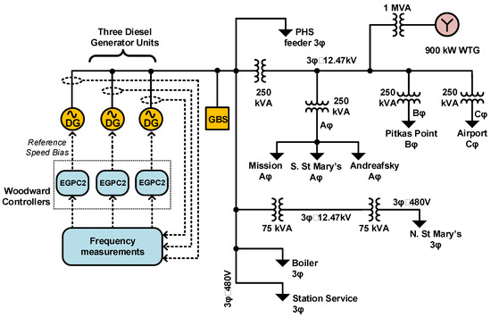
Figure 1.
Schematic of the Electrical Power System of St. Mary’s.
The models of the simulated loads were set to operate during peak demands in summer, with the load data gathered at the powerhouse on a multiple-year, and 15-minute time basis. The single and three phase loads were modeled as constant power loads. The load values are summarized in Table 1, where it can be noticed that the power system is unbalanced.

Table 1.
Used Load Values for Simulations.
In order to avoid voltage and current oscillations between the diesel gensets and the wind turbine, the line impedances of the simulation model must be included. This will keep the simulation model away from being underdamped. The estimation of the line impedances were obtained using 1/0# ACSR cable data while the transmission line lengths were acquired using satellite imagery. A summary of such line lengths is shown in Table 2. The values of the resistances used for the simulation model were: 0.54754 Ω/km and 0.3864 Ω/km for positive and zero-sequence, respectively. The values of the inductances used were: 0.001426 H/km and 0.0041264 H/km for positive and zero-sequence, respectively. Finally, the values of the capacitances used were: 1.235 nF/km and 7.751 nF/km for positive and zero-sequence, respectively [9].
Table 2.
Lengths of the Transmission Lines for the St. Mary’s Model.
2.2. Diesel Generator Model
In order to simplify simulation complexity, each of the diesel gensets were modeled using three parallel 600 kW units. Moreover, each genset model incorporates the corresponding prime mover, the exciter, and the governor. The prime mover was depicted using a SimScape Power Systems Synchronous Machine block [10], with an inertia constant of 0.4 s and 4 poles. The governor (DEGOV) was tailored from foregoing literature reviews [11,12]. The exciter was modeled using an AC4A-type exciter (which includes a voltage compensator gain of 200 V/V, and time constant of 0.015 s) [13]. The voltage set point to the AC4A exciter was obtained using a volt-var droop of 2%. Such a droop is characteristic, and is derived from Equation (1).
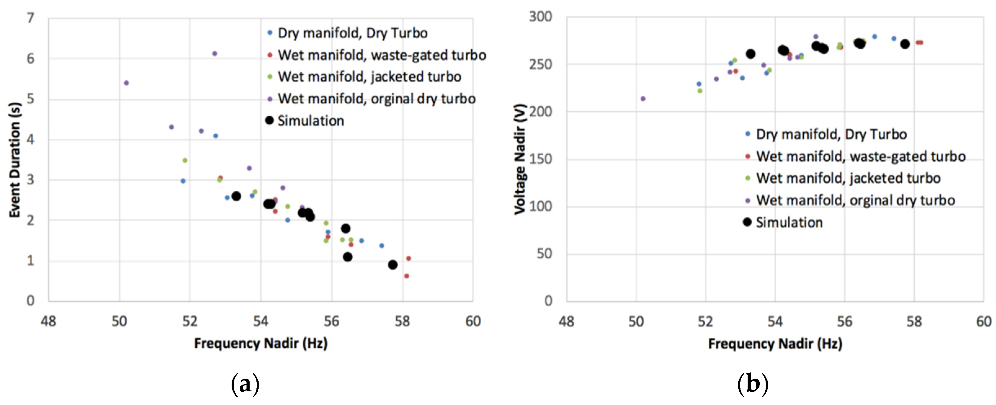
where, the variable Vref is the target voltage for the exciter; the variable Qeo is the reactive power (Var); and constant ηQ is the reactive power droop slope. For the tuning of the exciter and the governor to match the type of diesel generators utilized in St. Mary’s, the 600 kW generator model was corroborated against step load tests of different step sizes ranging from 100 to 300 kW. Such tests were performed by AVEC on a Detroit Diesel Series 60, 1800 RPM electronically regulated engine with diverse manifold (dry/wet) and turbo (jacketed/dry) conditions. The step load changes result in frequency/voltage deviations. The durations of these deviations were calculated as the time until any frequency deviations are less than 1% of nominal values. The simulated frequency/voltage nadirs and duration of the events match well with the experimental data over the range of conditions tested, as shown in Figure 2.
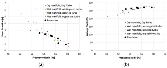
Figure 2.
MATLAB Simulations and AVEC’s Experimental Data at Varying Manifold and Turbo Conditions. (a) Event duration vs. frequency nadir. (b) Voltage nadir vs. frequency nadir.
So as to achieve balanced loading between the generators in such a way that the frequency is regulated to 60 Hz, the St. Mary’s model uses a Woodward EGCP2 regulator [14]. To characterize this control, a Frequency-Watt droop control scheme was employed to set the reference engine speed (ωref) on each of the governors. Based upon the sensed system’s frequency (f), the regulator sets the operating speed of the diesel engine (ωref) that is received by the governor. The governor block makes use of a PI regulator to equalize the speed of the engine (ω) to the reference speed (ωref), and outputs a mechanical power to the model of the diesel generator. The droop equation for the controller determines the correct reference speed for the governor as illustrated in Equation (2).
where, ωref is the target generator speed; ωnom is the nominal generator speed at 60 Hz; ηP is the frequency-watt droop slope (5%); fref is the target frequency (60 Hz); and f is the measured system frequency.
2.3. Wind Turbine Model
In order to mimic the dynamics of the EWT 900 kW wind turbine generator, an average-value model of a Type IV wind turbine was used [15]. Such model incorporates the following: a synchronous generator interfaced with a diode rectifier, a DC-DC PWM boost converter, and a DC/AC, IGBT-based PWM inverter. The actual model has a 2 MW wind turbine. To match the model to the EWT turbine used at St. Mary’s, the size of the synchronous generator was reduced proportionally from 2 MW to 900 kW. The power generation of the synchronous machine (Pgen) was suited to the wind speed function provided by EWT, and was fit using a 4th degree polynomial within the functional wind speed pattern of the EWT turbine (3–25 m/s), given by Equation (3). The modeled output power was saturated at a minimum limit of 0 p.u. and a maximum limit of 1 p.u. in the functional wind speed pattern.
where the variable v is the speed of the wind in m/s. The values of the coefficients k1 to k5 in Equation (3) are summarized in Equation (4).
Lastly, the original model underwent time constant modifications to pair with the ramp rates given by EWT (200 kW/s). The open circuit time constant of the d-axis (Tdo’) was reduced from 4.49 s in the original model to 0.49 s, whereas the inertia time constant was augmented from 0.62 s in the original model to 1.2 s. The aforementioned modifications permitted that the dynamics of a 1 p.u. step change match the dynamics of the EWT. The simulation results of the power output of the wind turbine were compared against data provided by EWT. As depicted in Figure 3, the wind speed output of the modeled wind turbine closely matches the data provided by EWT.
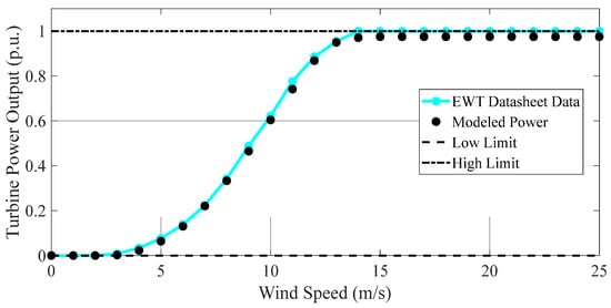
Figure 3.
Simulated Wind Power Vs. Wind Speed Curves Compared to Data Provided by EWT.
2.4. Grid-Forming Inverter Model
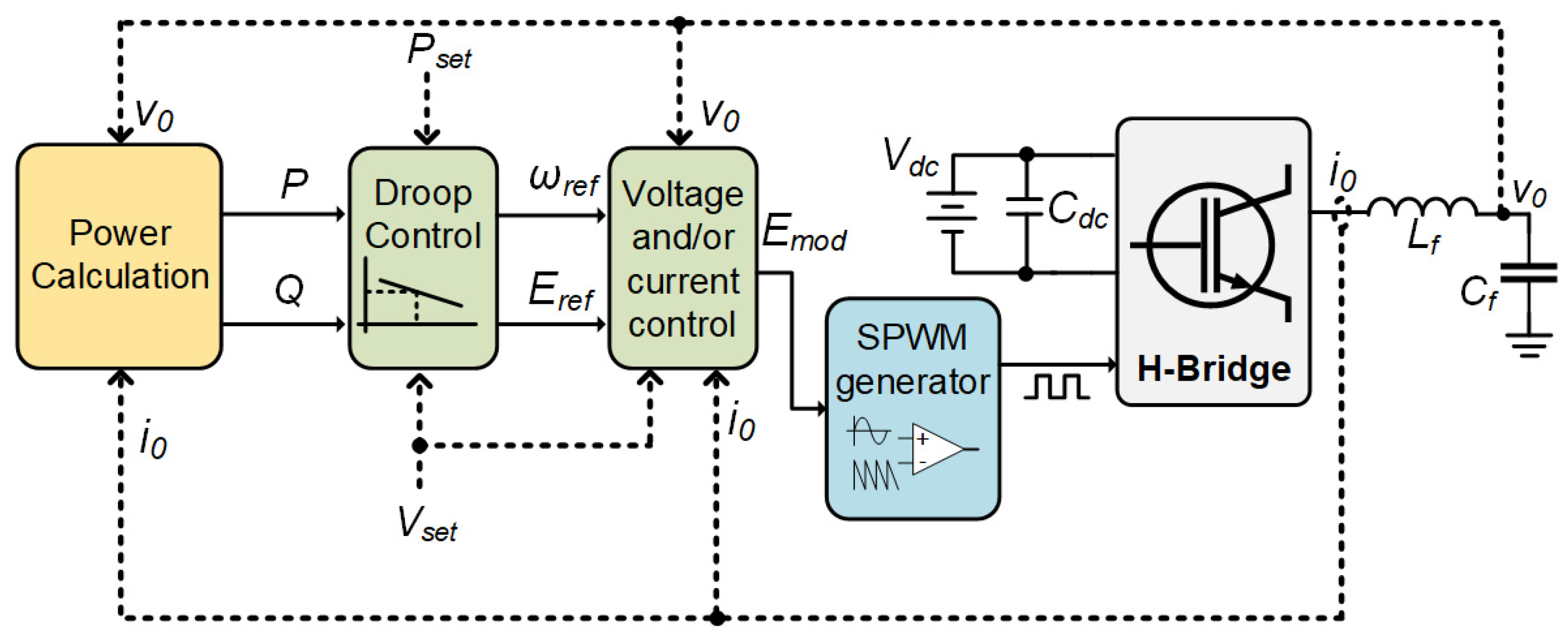
Two simulation models of GFMIs were used. Both have the same generic control scheme, as depicted in Figure 4, where the main dissimilarities relate to the current control and voltage regulation schemes that each model carries out.
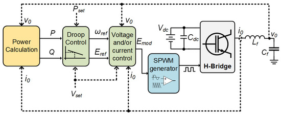
Figure 4.
Block Diagram for the Generic Control Scheme of a Grid-Forming Inverter.
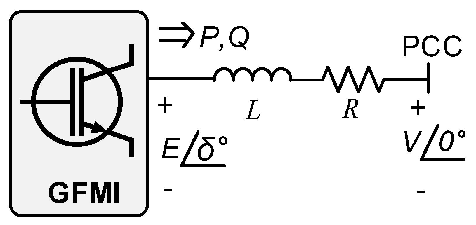
From Figure 4, notice that the droop characteristic in real and reactive power is a crucial section of the control scheme if the GFMIs are to share loads with other generation sources interconnected to the power system [16]. Figure 5 illustrates the diagram describing the power flow dynamics of the GFMI circuit.
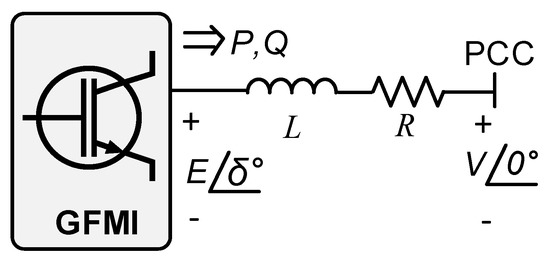
Figure 5.
Circuit Diagram Describing the Power Flow of a Grid-Forming Inverter.
Equations (5) and (6), which describe the droop characteristics, are based upon the power flow equations derived from the circuit depicted in Figure 5.
where E is the rms voltage at the inverter’s terminals, V is the rms voltage at PCC, and XL is the inductive coupling reactance between E and V. The accuracy of the approximations shown in Equations (5) and (6) are valid only in the case where the X/R ratio of the coupling impedance of the GFMI is adequately large (≈10), such that the resistor could be neglected [17]. When the X/R ratio is not sufficiently large, distinct droop characteristics are needed [18,19,20] to handle the low X/R ratio. Thus, if the linear behavior of the approximations in Equations (5) and (6) hold, the real power supplied by the inverter can be regulated only by the frequency droop, whereas the reactive power can be regulated only by the voltage droop, as illustrated in the f-P and Q-V droop linear plots depicted in Figure 6. The first GFMI model utilizes the CERTS grid-forming control scheme studied in [21], while the second model carries out voltage and current grid-forming control in the dq-frame [20], with the addition of a virtual impedance control loop, which ameliorates the internal stability of the GFMI [22]. The simulations in this work were performed in such a manner that the modulation index of the reference signals that controls the H-bridge of the GFMI operate in the linear region. Thus, the GFMI models were never driven to operate in their saturation modes (nonlinear modes).
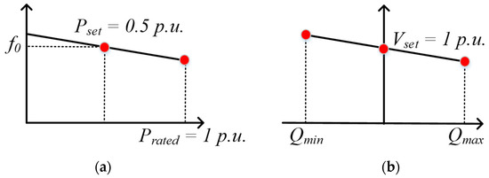
Figure 6.
Droop Characteristics Plots for the Generic Control Scheme of a GFMI. (a) f-P droop curve. (b) Q-V droop curve.
2.4.1. CERTS-Based Grid Forming Inverter Droop Control
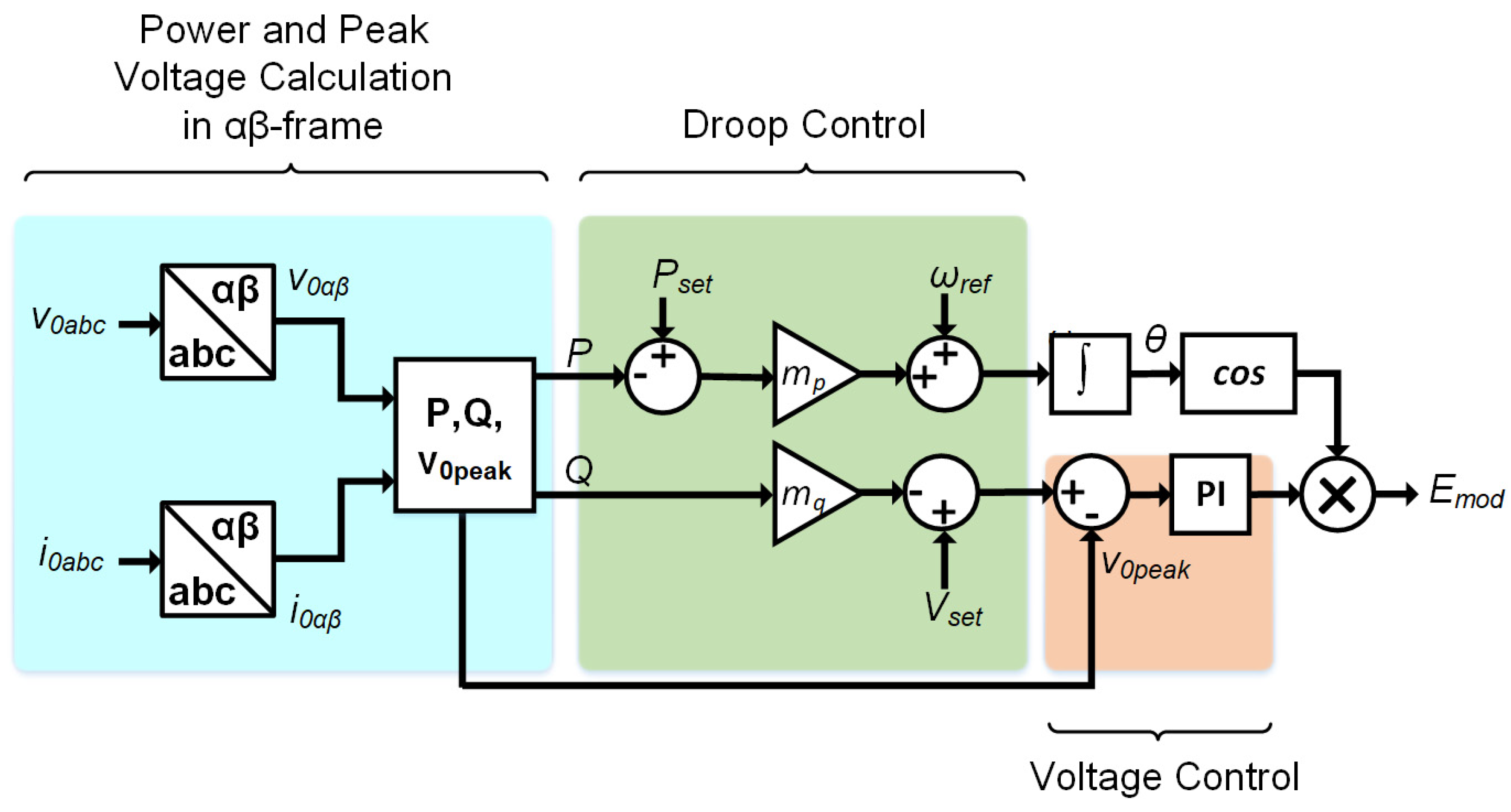
The block diagram describing the control scheme of the CERTS-based GFMI simulation model is shown in Figure 7. This scheme utilizes voltage and frequency-droop in order to regulate reactive and active power, respectively. Previous to the droop control scheme, the output signals of the current (i0) and the voltage (v0) are mapped into the stationary αβ-frame. Such transformed values of are utilized to determine active and reactive power, as per Equations (7) and (8), respectively [23].
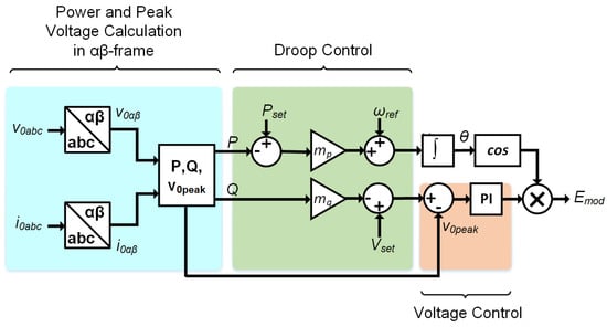
Figure 7.
Block Diagram for the CERTS GFMI Droop Control Model.
In the above equations, the variables and represent the alpha components of voltage and current, respectively; while the variables and represent their beta components. A Proportional-Integral (PI) regulator is used to control the output voltage of the GFMI according to the reference voltage set point given by the voltage droop stage. The use of such PI regulator aids in reducing any circulating currents that might be present in the system. The peak value of the output voltage provided to this PI regulator is calculated in the αβ-frame as per Equation (9).
A more complex CERTS-Based GFMI control scheme incorporates an overload mitigation controller, which aids in preventing the GFMI from a voltage collapse in the DC bus. Such a controller reduces the GFMI’s frequency in cases where it becomes overloaded [24]. To avoid complexity, the overload mitigation controller was ignored during simulations since proper precautions were taken to avoid overloading the GFMI under transient and steady state conditions.
2.4.2. DQ-Based Grid-Forming Inverter Model
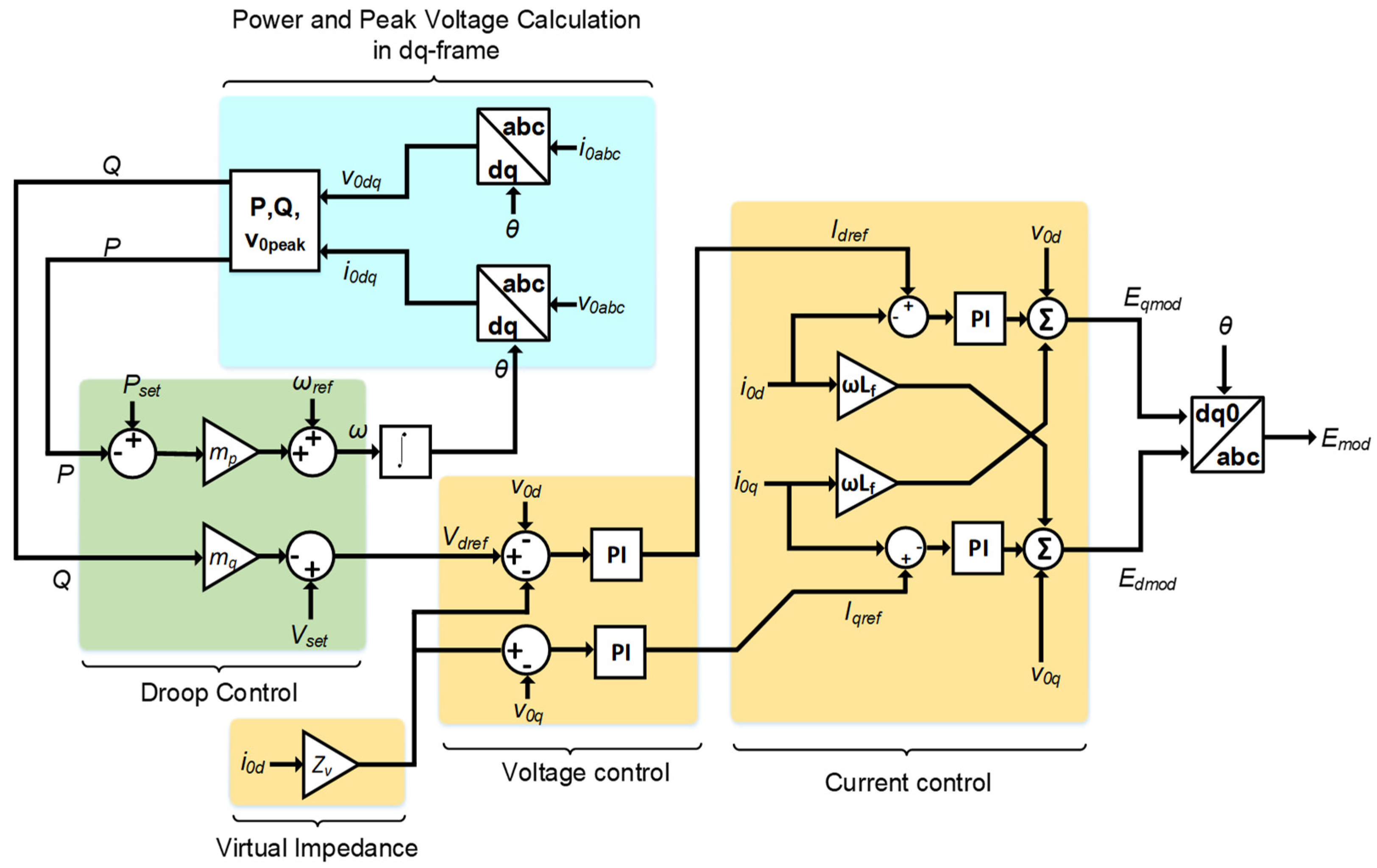
Figure 8 depics the control scheme for a dq-based GFMI model. Similarly to the CERTS model, the frequency-droop feature dictates the frequency of the system according to the real power demand. Nevertheless, this control scheme also uses the system’s angular displacement (θ) to obtain the dq-frame transformation of the output voltages and currents, which are used to compute the real and reactive power [23] using Equations (10) and (11), respectively:
where, vod and iod, are the d-components of the output voltages and currents of the GFMI, respectively; whereas, voq and ioq, are the corresponding q-components of the output voltages and currents, respectively. The voltage droop gives the d-component reference (Vdref) to the voltage PI regulator. Notice also the presence of a virtual impedance loop, which is useful in compensating for the intrinsic low X/R ratio of the transmission lines at distribution voltage levels [22]. Furthermore, the outputs of the voltage PI regulators set the references for the PI current regulators. As with the grid-following control schemes, the current control loops are the innermost in the regulation scheme, and thus, they provide the fastest response [25]. For this reason, the dynamics of the current regulators are programmed to one order of magnitude faster than the voltage regulators [25].
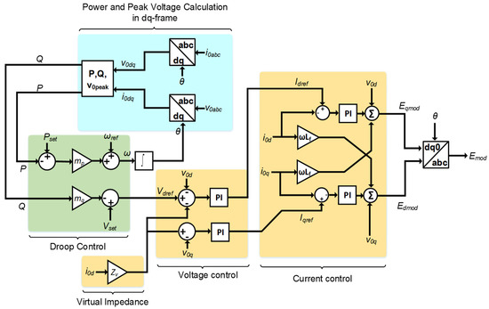
Figure 8.
Block Diagram for the Control Scheme of DQ-Based GFMI.
Due to the dq-transformation, the current control scheme must account and compensate for the transformation-generated current cross-coupling terms. The main purpose of this compensation is to decouple each current control loop from each other; which in turn, reduces the order of each current control loop to one single variable, facilitating and simplifying the current regulators design and stability analysis [23,25]. In addition, a voltage feedforward compensation is implemented in the current control scheme.
3. Power Hardware-in-the-Loop Setup
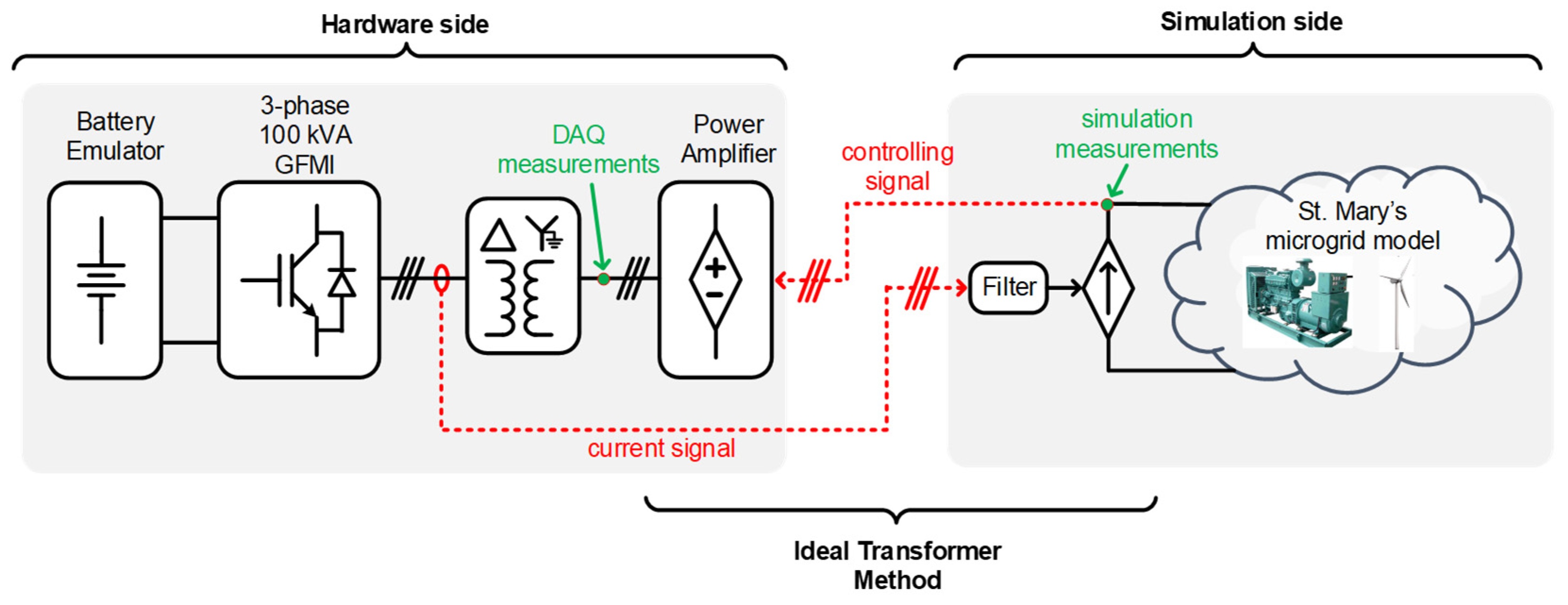
In order to validate and compare the dynamics of the simulations with the GFMI models, a PHIL setup was implemented using an ABB PCS-100, 100 kVA commercial GFMI. The schematic in Figure 9 shows the PHIL testbed, where the DC side of the GFMI is energized by a 100 kW, NHR (NH Research) battery emulator, whereas the AC side is connected to a 90 kVA Ametek, voltage-controlled AC power amplifier. The delta-wye grounded transformer provides isolation and protection to the GFMI against unstable transient dynamics that may occur inside the simulation model. There exist some challenges in connecting a GFMI to a voltage-controlled amplifier (grid simulator). The Ideal Transformer Method (ITM) is utilized [26] as the interface approach between the real-time simulation model and the ABB PCS-100 GFMI. For GFMIs without such a synchronization mechanism that normally operate in isochronous mode, the ITM is not suitable and a different interface method must be used, as proposed in [27]. The commercial ABB PCS-100 GFMI has two main operation modes, where each one has its own control modes [28]:
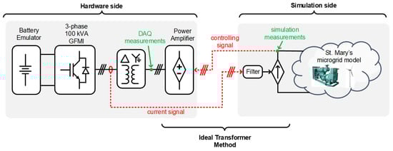
Figure 9.
Power Hardware-in-the-Loop Setup for Grid Forming Inverter Experimental Testing.
- (1)
- The Virtual Generator Mode (VGM), in which the GFMI interacts with the grid emulating a synchronous generator by presenting a low impedance voltage source to the grid. While on VGM, the GFMI can be operated in either: PQ power flow control, where the converter operates with set-points for active and reactive power; or Vf control, where the converter operates with fixed voltage and frequency set-points allowing islanding. Either of these two control modes can be selected while the GFMI is running.
- (2)
- The Current Source Inverter Mode (CSI), in which the GFMI presents a high-impedance current source to the grid and allowing only PQ control mode. Since no inertia is emulated, this operation mode is suitable for grid-tied support functions where sub-cycle response to power commands is required. It is important to point out that changing between VGM and CSI modes is not allowed while the GFMI is running.
4. Results and Discussion
To verify the aptness of the GBS to supply spinning reserve with 1, 2, or 3 diesel gensets, a loss of wind scenario was created in the simulation. Under this outline, the wind turbine reduces the supplied power steeply from 336 kW to 49 kW (65% of the total load to 9%). Even though the wind speed is presumed to descend instantaneously, rotors’ inertia limits the power rate of change to approximately 200 kW/s (obtained from data given by EWT), which means that the wind power descends from 336 kW to 49 kW in approximately 1.65 s.
4.1. Simulation Results of Each Grid-Forming Inverter Control Scheme
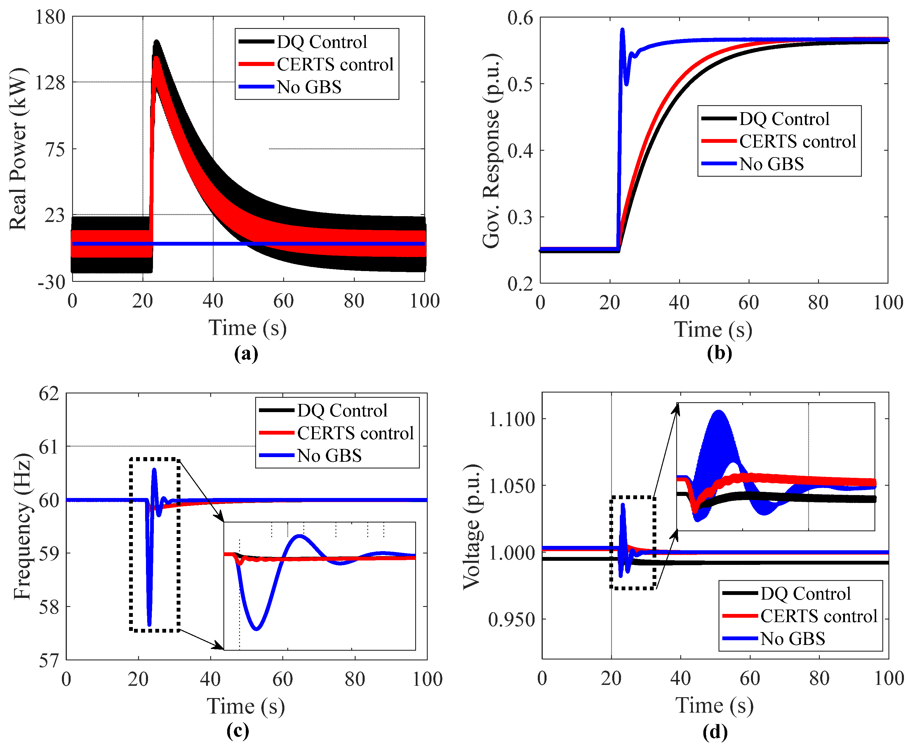
The dynamics of the two simulation models are compared without the use of PHIL devices. Simulation results of the St. Mary’s model are obtained with only one diesel generator operating. Both GFMI models were rated at 1 MVA with an operating voltage of 480 V. Figure 10 illustrates the simulation results obtained for: GBS active power, diesel generators governor response, system frequency, and voltage at the PCC when operating with and without the GFMI. The top row traces, Figure 10a,b, show the comparisons of the GBS output active powers of each GFMI control scheme and the system’s governor response, respectively. From Figure 10a, the GBS output active powers provided by the CERTS and DQ control schemes show very similar dynamics in terms of peak power and settling time. The thickened appearances of the power traces are due to the 120 Hz power ripple caused by the intrinsic unbalanced nature of the microgrid, which in this simulation is approximately 5%. The simulation results for the governor’s responses show that each control scheme has similar transient dynamics. From Figure 10b, notice how the absence of a GBS system causes and abrupt step-like response in the transient dynamics, which translates into a high fuel consumption of the diesel generators, whereas with the GBS present, the governor’s responses are smoothed out and the fuel consumption is reduced. Figure 10c,d depict the frequency and voltage dynamics of each GFMI control scheme, respectively. From the traces shown in Figure 10c and the magnified transient period, notice how the presence of the GBS system dampens the pronounced frequency nadir and frequency oscillations that occurred when the GBS system was not present. A similar dampening action is observed in the magnified transient portion of Figure 10d but acting over phase C voltage. Notice that the frequency and voltage responses of both control schemes have similar settling times.
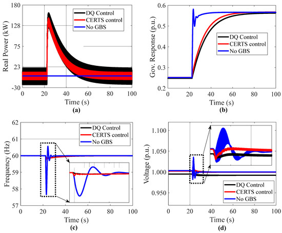
Figure 10.
Comparison of Two Grid-Forming Inverter Models under a Loss of Wind Scenario. (a) output power; (b) governor response; (c) systems’ frequency with magnified transient response; (d) output voltage of phase C with magnified transient response.
The use of the GBS to provide operating reserve notably reduces the speed of the response required from the diesel genset. This considerably reduces the fuel utilization of the generators while enhancing the frequency and voltage responses in terms of frequency nadir and voltage deviations, as depicted in Figure 11 and Figure 12, which also include traces for 2 and 3 generators online.

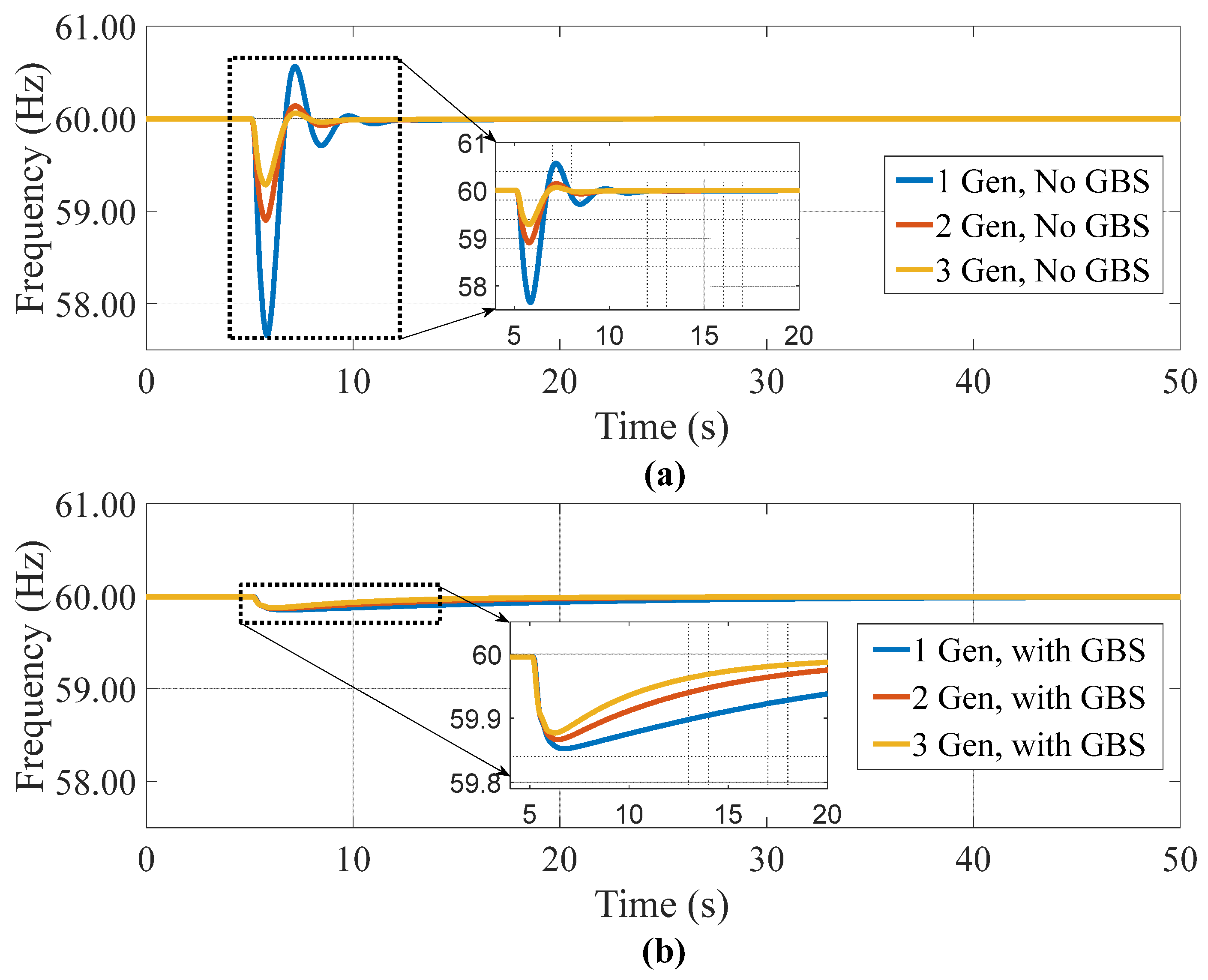
Figure 11.
Frequency Dynamics during a Loss of Wind Scenario under Different Number of Gensets. (a) Without GBS; (b) With GBS using DQ-control scheme.
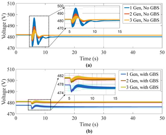
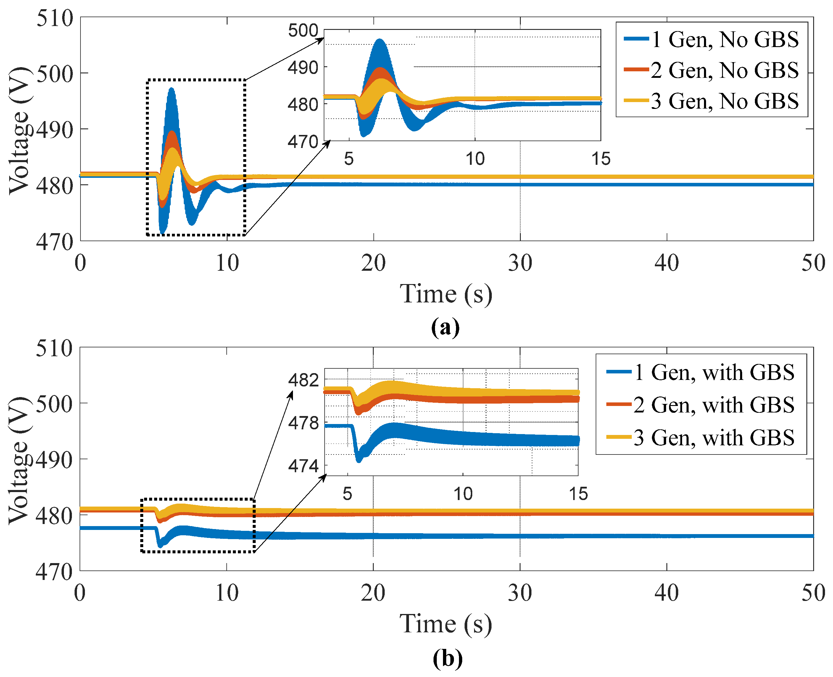
Figure 12.
Voltage Dynamics during Loss of Wind Scenario under Different Number of Generators. (a) Without GBS; (b) With GBS Using DQ-control-scheme.
Figure 11a illustrates the simulation results obtained for the system’s frequency without the GBS supplying spinning reserve for: one, two, and three-generator cases. The magnified portion of the transient period illustrates that the frequency nadir decreases as the number of generators increases. Figure 11b illustrates the simulation results obtained for the three diesel generator cases with the GBS providing spinning reserve along with a magnified portion of the transient period. Dissimilar to the diesel-only cases, the frequency nadir is substantially unrestrained from the number of generators in the system. This is because the frequency nadir is bounded by the speed of response of the GBS system. A larger GBS speed of response would result in a minor frequency deviation.
However, since the GBS is already operating at its maximum ramp rate and governs the output of real power near the deviation, modifications in the number of gensets do not have a noteworthy impact in the frequency nadir. Similarly, Figure 12 depicts the phase C voltage at the PCC of the powerhouse. In the absence of a GBS, Figure 12a shows that the voltage deviation decreases as the number of generators increases. However, when the GBS is present and providing spinning reserve, as depicted in Figure 12b, the voltage deviation is independent of the number of generators operating in the system. This is because the voltage behavior is dominated by the GBS, which provides voltage regulation at its maximum ramp rate. The results for the frequency nadir and voltage deviations are summarized in Figure 13.

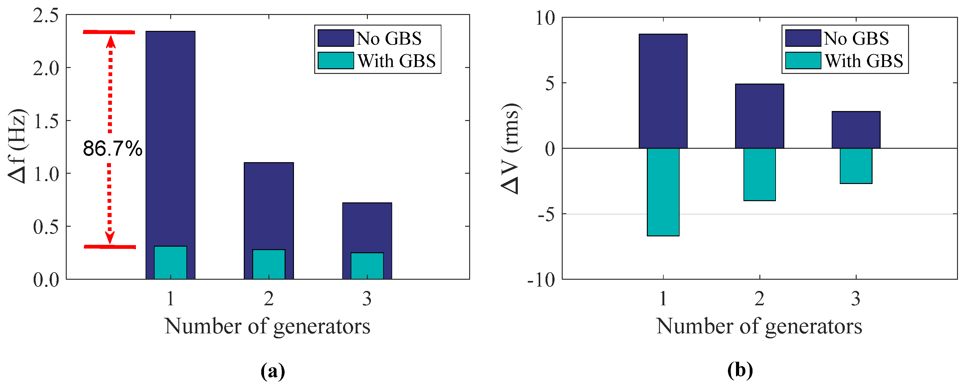
Figure 13.
Comparison of Voltage and Frequency Nadir for Different Combinations of Generators Considering Scenarios with and without the GBS. (a) Frequency nadir. (b) Voltage deviation.
From Figure 13a. When only one generator is online, notice that the presence of the GBS reduces the frequency nadir by 86.7%. For the cases of two and three generators online, the frequency nadirs were reduced by 74.55% and 65.28%, respectively. From Figure 13b, notice that the voltage deviations with the GBS present have opposite polarity as compared with the voltage deviations without GBS. However, when only one generator is online, the absolute value of the magnitude of the voltage deviation is reduced by 3.57%. For the cases of two and three generators online, the voltage deviations were reduced by 18.37% and 23%, respectively.
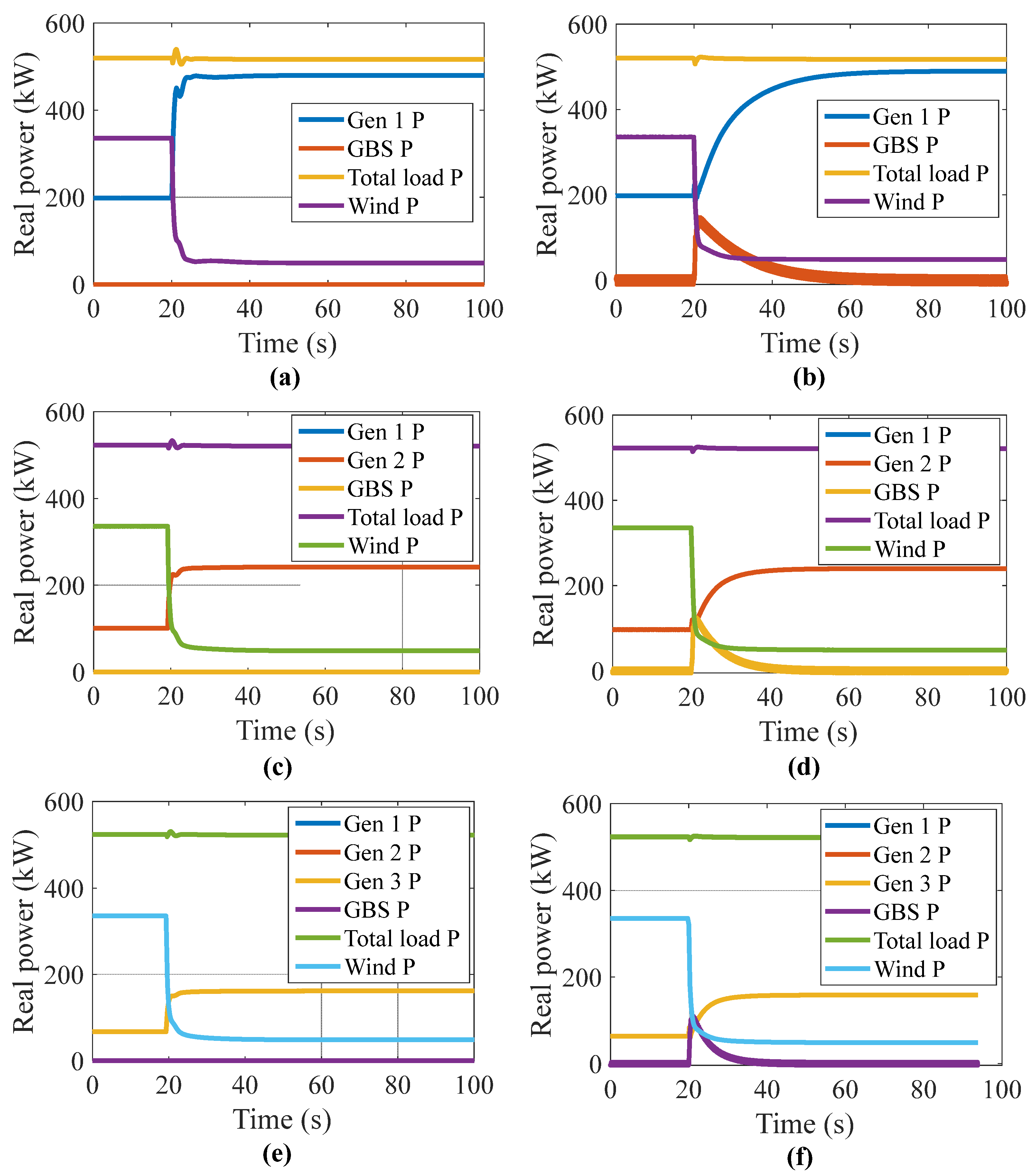
Furthermore, Figure 14 illustrates the simulation results obtained for the active power traces for the different generator cases when the system is subjected to a loss of wind turbine generation.
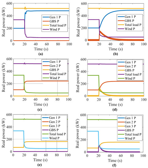
Figure 14.
Active Power Traces for Different Generator Cases with a Loss of Wind Scenario. (a) One Diesel generator. (b) One diesel generator and a grid-forming inverter. (c) Two diesel generators. (d) Two diesel generators and a grid-forming inverter. (e) Three diesel generators. (f) Three diesel generators and a grid-forming inverter.
Figure 14a,b illustrate the simulation results obtained for the response of the St. Mary’s system without and with the GBS, respectively. Figure 14c,d illustrate the simulation results obtained for the response of the St. Mary’s system operating with two diesel generators without and with the GBS, respectively. Finally, Figure 14e,f illustrate the simulation results obtained for the response of the St. Mary’s system operating with three diesel generators without and with the GBS, respectively.
4.2. Power Hardware-in-the-Loop Experimental Results
To test the dynamic responses of a physical GFMI, a commercial three-phase GFMI is integrated into the St. Mary’s simulation model in order to perform PHIL experimental tests. The GFMI used is the ABB PCS100, rated 100 kW at 380. A physical 380/480 V (delta-wye grounded) transformer is connected at the terminals of the ABB PCS100 GFMI.
The experimental results shown in Figure 15 demonstrate the incorporation of the ABB PCS100 in the PHIL simulation as the GBS, which is operated in PQ mode in the simulated St. Mary’s system with the three diesel generators online. The GBS system is ramped to real power values of: 0.2, 0.4, 0.5, and 0.75 p.u, held at 0.75 p.u and then ramped to zero.
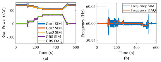
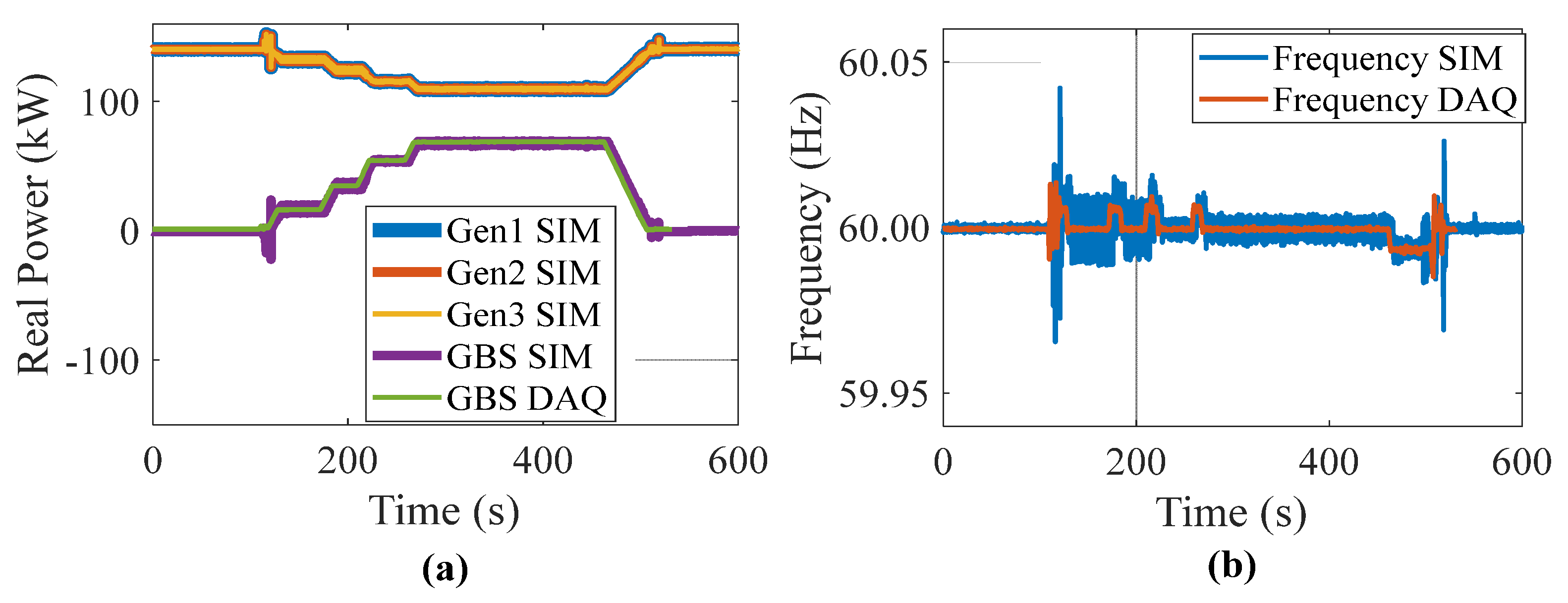
Figure 15.
Results from the PHIL incorporation of 100 kW ABB PCS100 operated in VGM-PQ mode. (a) Comparison between the power output vs. time for the simulated generators and the GBS and the real power flow measured in the laboratory DAQ data. (b) Comparison between system’s frequency vs. time for the simulated and laboratory DAQ data.
Figure 15a illustrates the internal simulation measurements for the diesel generators as well as a comparison between the simulation and the laboratory data acquisition system (DAQ) measurements for the real power flow from the GBS. This comparison illustrates that as the GBS real power ramps up, the real power provided by the diesel generators ramp down in order to keep the overall power of the system at a constant and the frequency at nominal 60 Hz.
Figure 15b illustrates a comparison between the simulation and laboratory DAQ measurements for the frequency of the GBS. These two frequency traces shown an excellent agreement that even replicates the slight increase in frequency as the GBS ramps up before the droop control of the generators re-asserts the frequency to 60 Hz through a ramp down of the generator output. The comparison between simulated and measured results illustrated in Figure 15 shows the power injection into the St. Mary’s system at powers up to 0.75 p.u. (75 kW). However, the proposed system at St. Mary’s will be a 1 MW system. In order to replicate the behavior of a 1 MW system with the physical 100 kW GFMI in the laboratory, it is necessary to scale the power injected by the commercial GFMI by a factor of ten. This scaling is typically performed by adding a proportionality constant to the current injection of the digital twin inside of the simulation model. This allows for emulation of larger units in simulation than exists in hardware. The main drawback with this scaling technique is that superimposed noise in the current signals is amplified. Furthermore, if an isolation transformer, such as the one shown in Figure 9, is used, the highly distorted magnetization currents are also amplified. The amplification of highly distorted feedback currents can lead to PHIL instability, which in turn can cause catastrophic damage to the power equipment involved.
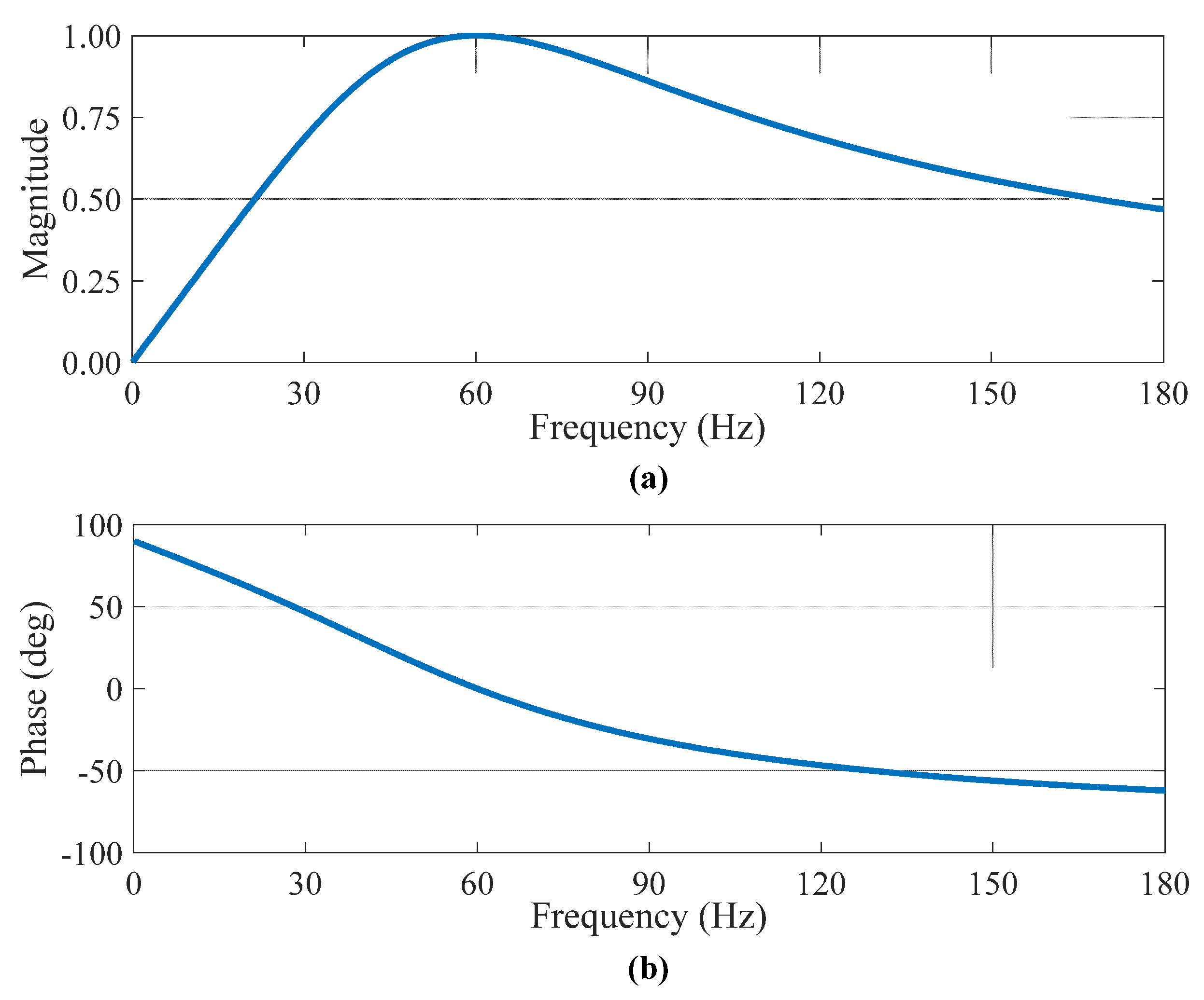
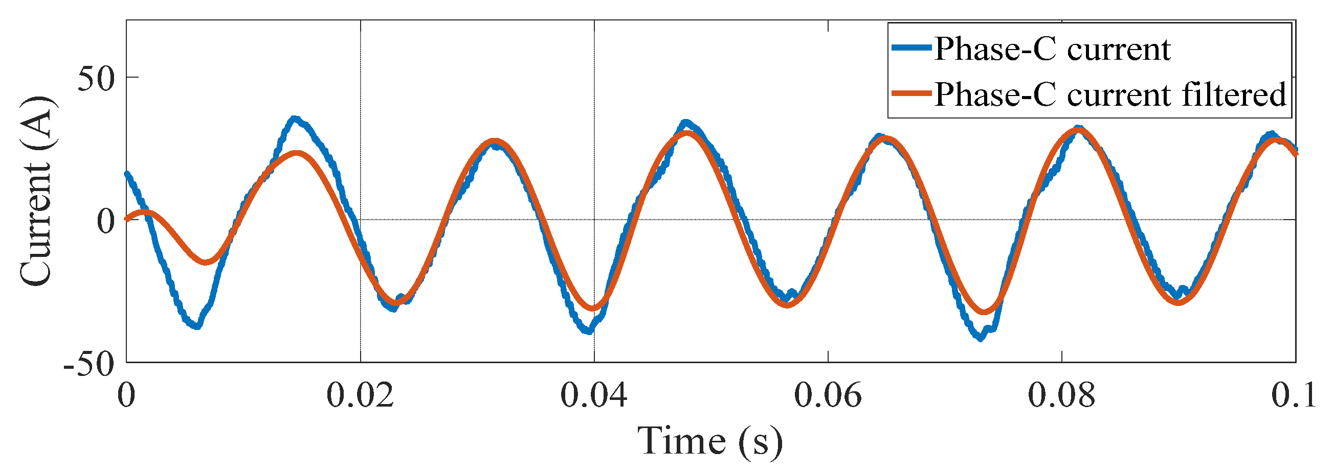
In order to filter out the magnetization current noise, a second order band-pass filter was placed in the simulation model. One of the main advantages of the band-pass filter is that for frequencies at the mid-band (i.e., 60 Hz), the phase lag due to the filter is zero degrees, as shown in Figure 16. This indicates that implementation of a band-pass filter will not affect the phase angle of the waveform and, therefore, no lead compensation block is necessary to re-synchronize the measured waveform before and after filtering. Figure 17 shows the results of implementing the band-pass filter on the measured current. The resultant waveform is significantly better behaved with little magnetization current and noise.
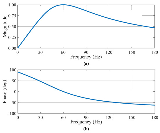
Figure 16.
Frequency Response of the Band-Pass Filter Placed in the Power Hardware-in-the-Loop Simulation Model. (a) Magnitude plot. (b) Phase plot.
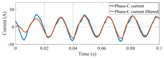
Figure 17.
Comparison Between the Unscaled PCS100 Phase C Current Before and After Filtering with the Band-Pass Filter.
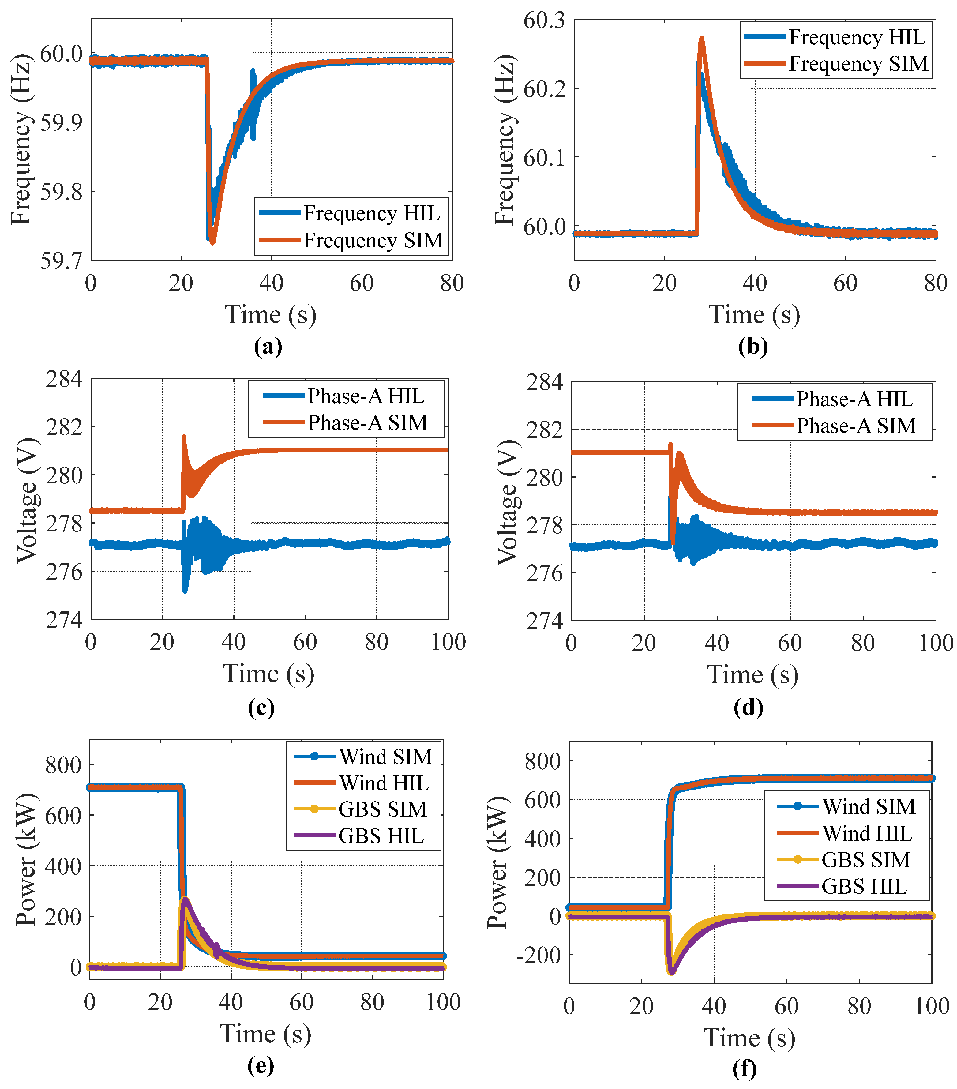
A PHIL simulation was carried out for a loss-of-wind scenario with a bank of three generators and the GBS in VGM-Vf mode to provide spinning reserve. In this scenario, the wind power drops from a value of 700 kW to 50 kW over a period of three seconds. Previous simulation-only results showed an expected frequency deviation in this instance of 0.7 Hz without a GBS present and 0.25 Hz with the GBS present. Figure 18 demonstrates the results obtained for the loss-of-wind scenarios for a bank of three generators and the GBS in simulation only using the VGM-Vf control scheme, and GBS in PHIL. The frequency drop shown in Figure 18a is due to the loss-of-wind. This is followed by a symmetrical increase in wind, which results in a subsequent frequency rise. The frequency traces show good agreement between pure simulation and PHIL with a frequency deviation of around 0.25 Hz in both instances. There is a minor mismatch in the voltage traces (Figure 18b) between the simulation and PHIL. The first difference is a slightly higher steady state voltage in simulation than is observed in PHIL. This can introduce a small voltage offset corresponding to the losses of the transformer. Moreover, in PHIL after the loss-of-wind transient, the voltage reasserts to its steady state value. This is compared to the simulation which has a slightly higher voltage after the wind transient. This is most likely due to a secondary voltage loop that is present in the ABB PCS100 control scheme that re-biases the voltage droop control back to the nominal value. Although the simulated GBS has a voltage droop, it does not contain a secondary loop to re-assert a nominal voltage level in steady state.
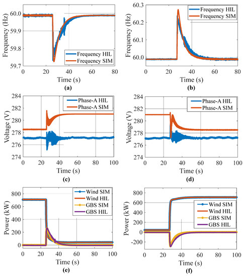
Figure 18.
Comparison between Simulation and Experimental Results. (a) Frequency for loss of wind. (b) Frequency for increase in wind. (c) Voltage for loss of wind. (d) Voltage for increase in wind. (e) Active power for loss of wind. (f) Active power for increase in Wind.
Notice from the comparison of the simulated GBS and experimental ABB PCS100 PHIL power output profile results have similar curves, as shown in Figure 18c. The power output of the ABB PCS100 shows a slightly longer extent in time of power output until the power decays back to zero. This affects the generator output by slowing its ramp to full power. This difference in time scale of power output can easily be replicated in simulation by altering the constants in the control loop for power output.
The results from the test system illustrate that there is a correlation between the simulated results using a simulation model of a GFMI and the experimental results obtained from a commercial GFMI using the PHIL testbed. These results also demonstrate that the GBS as spinning reserve provides significant frequency and voltage stability compared to relying only on diesel generation. These results show that the use of GBS could potentially help in reducing the necessary diesel generation units that provide spinning reserve from three down to one without sacrificing power quality. In summary, the simulation and the PHIL results with a commercial GFMI show excellent agreement for a loss-of-wind scenario with slight changes in the control scheme time constants to accurately represent the power output of the GFMI providing spinning reserve. These results demonstrate the stability of the system and the ability to simulate a 1 MW GBS system in St. Mary’s.
5. Conclusions
The ability of a battery-backed GBS to provide spinning reserve and voltage stability in a hybrid microgrid is demonstrated in this paper. The GBS was tested using a high-fidelity simulation model of an actual hybrid microgrid located in the region of St. Mary’s, Alaska. In order to disrupt voltage and frequency dynamics, a loss-of-wind scenario was simulated. Simulation-only results show that if the GBS is incorporated, the dynamics of the system are improved compared to using only diesel gensets as spinning reserve inside the microgrid’s powerhouse. Such improvements were observed in the form of: (i) smooth frequency nadir and response, causing the governor’s dynamics to slow down and reducing fuel consumption, which is a significant benefit for remote communities where the energy costs are high due to the high fuel transportation prices; (ii) faster voltage arresting and voltage regulation, which improves the resiliency of the system. It was also observed that the grid-forming capability of the GBS helped to dampen the frequency and voltage oscillations shown during the loss-of-wind scenario when only diesel gensets were used.
For the cases where three diesel generators were operating, when incorporating the GFMI there was an improvement in frequency nadir reduction of 65.28% and in voltage deviation of 3.57%. When considering the case of two diesel generators, there was a reduction in frequency nadir of 74.55% and in voltage deviation of 18.37%. Finally, for the case with only one diesel generator, there was a frequency nadir reduction of 86.75% and in voltage deviation of 22.99%. These results show that adding a GFMI reduced the frequency nadir and voltage deviation. The use of PHIL, which incorporated a commercially available 100kVA GFMI, helped to validate the obtained frequency nadir and voltage deviation results. These PHIL experiments provide a glimpse into GFMI dynamics that could be critical before deploying these systems into the field.
Author Contributions
Conceptualization, J.H.-A. and J.D.F.; methodology, J.H.-A. and J.D.F.; software and simulation modelling, J.H.-A. and J.D.F.; validation, J.H.-A., J.D.F. and R.D.-Z.; formal analysis, J.H.-A. and J.D.F.; investigation, J.H.-A.; resources, J.H.-A.; data curation, J.H.-A. and R.D.-Z.; writing—original draft preparation, J.H.-A., J.D.F. and R.D.-Z.; writing—review and editing, J.H.-A., R.D.-Z., J.D.F., M.S., W.T. and J.V.; visualization, J.H.-A., R.D.-Z. and J.D.F. supervision, J.D.F.; project administration, J.D.F.; funding acquisition, J.D.F. All authors have read and agreed to the published version of the manuscript.
Funding
This work was sponsored by the Department of Energy Office of Electricity Delivery & Energy Reliability under Contract No. NA0003525 work order numbers 35155, 16872, 31722, 33833 under the “Alaska St. Mary’s” project within the Renewable Energy & Distributed Systems Integration sub-sub program at Sandia National Laboratories.
Acknowledgments
Sandia National Laboratories is a multi-mission laboratory managed and operated by National Technology and Engineering Solutions of Sandia, LLC, a wholly owned subsidiary of Honeywell International, Inc., for the U.S. Department of Energy’s National Nuclear Security Administration under contract DE-NA-0003525. The authors acknowledge the support provided by Matthew J. Reno, Sigifredo Gonzalez and Nicholas S. Gurule.
Conflicts of Interest
The authors declare no conflict of interest.
References
- Holdmann, G.P.; Wies, R.W.; Vandermeer, J.B. Renewable Energy Integration in Alaska’s Remote Islanded Microgrids: Economic Drivers, Technical Strategies, Technological Niche Development, and Policy Implications. Proc. IEEE 2019, 107, 1820–1837. [Google Scholar] [CrossRef]
- Katiraei, F.; Iravani, R.; Hatziargyriou, N.; Dimeas, A. Microgrids management. IEEE Power Energy Mag. 2008, 6, 54–65. [Google Scholar] [CrossRef]
- Du, W.; Tuffner, F.K.; Schneider, K.P.; Lasseter, R.H.; Xie, J.; Chen, Z.; Bhattarai, B. Modeling of Grid-Forming and Grid-Following Inverters for Dynamic Simulation of Large-Scale Distribution Systems. IEEE Trans. Power Deliv. 2021, 36, 2035–2045. [Google Scholar] [CrossRef]
- Lasseter, R.H.; Piagi, P. Microgrid: A Conceptual Solution. In Proceedings of the 2004 IEEE 35th Annual Power Electronics Specialists Conference, Aachen, Germany, 20–25 June 2004. [Google Scholar]
- Rosso, R.; Wang, X.; Liserre, M.; Lu, X.; Engelken, S. Grid-Forming Converters: Control Approaches, Grid-Synchronization, and Future Trends—A Review. IEEE Open J. Ind. Appl. 2021, 2, 93–109. [Google Scholar] [CrossRef]
- Milano, F.; Dorfler, F.; Hug, G.; Hill, D.J.; Verbič, G. Foundations and challenges of low-inertia systems. In Proceedings of the 20th Power Systems Computation Conference, PSCC 2018, Dublin, Ireland, 11–15 June 2018. [Google Scholar]
- Hernandez-Alvidrez, J.; Gurule, N.S.; Darbali-Zamora, R.; Reno, M.J.; Flicker, J.D. Modeling a Grid-Forming Inverter Dynamics under Ground Fault Scenarios Using Experimental Data from Commercially Available Equipment. In Proceedings of the Conference Record of the IEEE Photovoltaic Specialists Conference, Fort Lauderdale, FL, USA, 20–25 June 2021; pp. 1517–1523. [Google Scholar]
- Markovic, U.; Stanojev, O.; Aristidou, P.; Vrettos, E.; Callaway, D.; Hug, G. Understanding Small-Signal Stability of Low-Inertia Systems. IEEE Trans. Power Syst. 2021, 36, 3997–4017. [Google Scholar] [CrossRef]
- Nexans. Bare Overhead Conductors: AAC, ACSR, ACSR II. 2003. Available online: http://www.docdatabase.net/more-bare-overhead-conductors-nexans-usa-1275046.html (accessed on 7 September 2020).
- Sybille, G.; Brunelle, P.; Giroux, P.; Casoria, S.; Gagnon, R.; Kamwa, I.; Roussel, R.; Chamagne, R.; Dessaint, L.; Lehuy, H. SimPowerSystems for Use with Simulink; Mathworks: Natick, MA, USA, 2003. [Google Scholar]
- Sybille, G.; Zabaiou, T. Emergency Diesel-Generator and Asynchronous Motor. 2018. Available online: https://www.mathworks.com/help/physmod/sps/examples/emergency-diesel-generator-and-asynchronous-motor.html (accessed on 1 February 2022).
- Yeager, K.; Willis, J.R. Modeling of emergency diesel generators in an 800 megawatt nuclear power plant. IEEE Trans. Energy Convers. 1993, 8, 433–441. [Google Scholar] [CrossRef]
- Zabaiou, T.; Dessaint, L.A.; Brunelle, P. Development of a new library of IEEE excitation systems and its validation with PSS/E. In Proceedings of the IEEE Power and Energy Society General Meeting, San Diego, CA, USA, 22–26 July 2012. [Google Scholar]
- Woodward Inc. EGCP-2 Genset Controller. Available online: http://www.woodward.com/egcp2.aspx (accessed on 1 February 2022).
- Gagnon, R.; Brochu, J. Wind Farm—Synchronous Generator and Full Scale Converter (Type 4) Detailed Model. 2016. Available online: https://www.mathworks.com/help/physmod/sps/examples/wind-farm-synchronous-generator-and-full-scale-converter-type-4-detailed-model.html (accessed on 1 February 2022).
- Hernandez-Alvidrez, J.; Summers, A.; Reno, M.J.; Flicker, J.; Pragallapati, N. Simulation of Grid-Forming Inverters Dynamic Models using a Power Hardware in the Loop Testbed. In Proceedings of the 46th IEEE Photovoltaic Specialists Conference, Chicago, IL, USA, 16–24 June 2019. [Google Scholar]
- Kundur, P. Power System Stability and Control; Tata McGraw-Hill: New York, NY, USA, 1993. [Google Scholar]
- Bevrani, H.; François, B.; Ise, T. Microgrid Dynamics and Control; Wiley & Sons: Hoboken, NJ, USA, 2017. [Google Scholar]
- Bidram, A.; Nasirian, V.; Davoudi, A.; Lewis, F.L. Cooperative Synchronization in Distributed Microgrid Control, 1st ed.; Springer: Berlin/Heidelberg, Germany, 2017. [Google Scholar]
- Vinayagam, A.; Swarna, K.S.V.; Khoo, S.Y.; Oo, A.T.; Stojcevski, A. PV Based Microgrid with Grid-Support Grid-Forming Inverter Control-(Simulation and Analysis). Smart Grid Renew. Energy 2017, 8, 1–30. [Google Scholar] [CrossRef] [Green Version]
- Du, W.; Schneider, K.P.; Tuffner, F.K.; Chen, Z.; Lasseter, R.H. Modeling of Grid-Forming Inverters for Transient Stability Simulations of an all Inverter-based Distribution System. In Proceedings of the 2019 IEEE Power & Energy Society Innovative Smart Grid Technologies Conference, Washington, DC, USA, 18–21 February 2019; pp. 1–5. [Google Scholar]
- Yao, W.; Chen, M.; Matas, J.; Guerrero, J.M.; Qian, Z.M. Design and analysis of the droop control method for parallel inverters considering the impact of the complex impedance on the power sharing. IEEE Trans. Ind. Electron. 2011, 58, 576–588. [Google Scholar] [CrossRef]
- Yazdani, A.; Iravani, R. Voltage-Sourced Converters in Power Systems: Modeling, Control, and Applications; IEEE Press: Piscataway, NJ, USA; John Wiley: Hoboken, NJ, USA, 2010. [Google Scholar]
- Du, W.; Lasseter, R.H.; Khalsa, A.S. Survivability of autonomous microgrid during overload events. IEEE Trans. Smart Grid 2019, 10, 3515–3524. [Google Scholar] [CrossRef]
- Teodorescu, R.; Liserre, M.; Rodríguez, P. Grid Converters for Photovoltaic and Wind Power Systems; Wiley: Hoboken, NJ, USA, 2011. [Google Scholar]
- Summers, A.; Hernandez-Alvidrez, J.; Darbali-Zamora, R.; Reno, M.J.; Johnson, J.; Gurule, N.S. Comparison of Ideal Transformer Method and Damping Impedance Method for PV Power-Hardware-In-The-Loop Experiments. In Proceedings of the Conference Record of the IEEE Photovoltaic Specialists Conference, Chicago, IL, USA, 19–21 June 2019; pp. 2989–2996. [Google Scholar]
- Hernandez-Alvidrez, J.; Gurule, N.S.; Reno, M.J.; Flicker, J.D.; Summers, A.; Ellis, A. Method to Interface Grid-Forming Inverters into Power Hardware in the Loop Setups. In Proceedings of the 47th IEEE Photovoltaic Specialists Conference, Calgary, AB, Canada, 15 June–21 August 2020. [Google Scholar]
- ABB. PCS100 ESS Grid Connect Interface for Energy Storage Systems User Manual, 1st ed.; Available online: https://cdn2.hubspot.net/hubfs/1828458/Website%20downloads/Brochures/Battery/Product%20Brochure%20-%20ABB%20PCS%20-%20Spirit%20Energy%20.pdf (accessed on 1 February 2022).


Publisher’s Note: MDPI stays neutral with regard to jurisdictional claims in published maps and institutional affiliations. |
© 2022 by the authors. Licensee MDPI, Basel, Switzerland. This article is an open access article distributed under the terms and conditions of the Creative Commons Attribution (CC BY) license (https://creativecommons.org/licenses/by/4.0/).