Author Contributions
Conceptualization, R.D.-R. and I.B.; methodology, R.D.-R.; software, R.D.-R., M.M. and I.B.; validation, R.D.-R., G.R. and M.M.; formal analysis, R.D.-R. and G.R.; investigation, R.D.-R. and I.B.; resources, R.D.-R., G.R. and M.M.; data curation, I.B. and R.D.-R.; writing—original draft preparation, I.B., R.D.-R., G.R. and M.M.; writing—review and editing, I.B., R.D.-R., G.R. and M.M.; visualization, R.D.-R., I.B., M.M. and G.R.; supervision, R.D.-R.; project administration, R.D.-R.; funding acquisition, R.D.-R. All authors have read and agreed to the published version of the manuscript.
Figure 1.
Polyurethane foam laminas. This image illustrates the setting of three superimposed laminas clamped with a vice. The thickness of each lamina is 3.3 mm, and the total thickness of the three laminas all together was ±10 mm.
Figure 1.
Polyurethane foam laminas. This image illustrates the setting of three superimposed laminas clamped with a vice. The thickness of each lamina is 3.3 mm, and the total thickness of the three laminas all together was ±10 mm.
Figure 2.
Drill tip angles. Composition image of the four drill tips used in this experiment. (A) Anker tapered drill tip, angle: 93 degrees; (B) Megagen tapered drill tip, angle: 98 degrees; (C) Nobel Biocare tapered drill tip, angle: 108 degrees; and (D) Densah tapered drill tip, angle: 120 degrees.
Figure 3.
Drill wall angles. Composition image of the four drills used in this experiment. (A) Anker tapered drill walls, angle: 13 degrees; (B) Megagen tapered drill walls, angle: 5 degrees; (C) Nobel Biocare Tapered drill walls, angle: 7 degrees; and (D) Densah tapered drill walls, angle: 3 degrees.
Figure 4.
Image of processing for measuring. (A) Implant bed wall region of interest marked with a polygon. (B) Transformation in an 8-bit image. (C) Thresholding of the region of the interest based on the pixel color. (D) Region of interest structured and measured.
Figure 4.
Image of processing for measuring. (A) Implant bed wall region of interest marked with a polygon. (B) Transformation in an 8-bit image. (C) Thresholding of the region of the interest based on the pixel color. (D) Region of interest structured and measured.
Figure 5.
Volume reconstruction for the qualitative evaluation of the microarchitecture. Scanning was completed in a volume of 10 mm × 10 mm. This is a 3D image of the coronal section of the Densah burs group in counterclockwise drilling.
Figure 5.
Volume reconstruction for the qualitative evaluation of the microarchitecture. Scanning was completed in a volume of 10 mm × 10 mm. This is a 3D image of the coronal section of the Densah burs group in counterclockwise drilling.
Figure 6.
Figure composition showing representative samples of 2D sections at the coronal region for clockwise and counterclockwise drilling for all of the drill designs. Clockwise and counterclockwise drilling produced microfractures of the implant bed walls. Some localized thickening was observed in both drilling directions. However, wall density was not increased in any of the drilling directions.
Figure 7.
Box plot for the percentage of bone condensation at the coronal area for all groups. C = clockwise drilling; T = counterclockwise drilling. The Anker drill group showed a lower mean value; however, the statistical analysis did not show significant differences.
Figure 7.
Box plot for the percentage of bone condensation at the coronal area for all groups. C = clockwise drilling; T = counterclockwise drilling. The Anker drill group showed a lower mean value; however, the statistical analysis did not show significant differences.
Figure 8.
Figure composition showing representative samples of 2D sections at the middle region for clockwise and counterclockwise drilling for all of the drill designs. Microfractures were observed in all the implant bed walls. Some of the empty spaces of the cancellous area were exposed to the implant bed intaglio. Wall density appeared the same for both drilling directions.
Figure 9.
Box plot for the percentage of bone condensation at the middle area for all groups. C = clockwise drilling; T = counterclockwise drilling.
Figure 9.
Box plot for the percentage of bone condensation at the middle area for all groups. C = clockwise drilling; T = counterclockwise drilling.
Figure 10.
Figure composition showing representative samples of 2D sections at the apical region. Both groups showed slightly increased density at the apical area in clockwise rotation. The counterclockwise drilling showed the highest bone density for all of the drill designs.
Figure 10.
Figure composition showing representative samples of 2D sections at the apical region. Both groups showed slightly increased density at the apical area in clockwise rotation. The counterclockwise drilling showed the highest bone density for all of the drill designs.
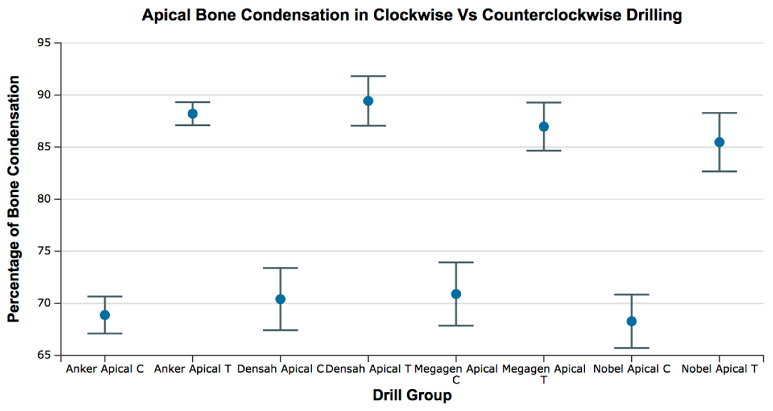
Figure 11.
Box plot for the percentage of bone condensation at the apical area for all groups. C = clockwise drilling; T = counterclockwise drilling.
Figure 11.
Box plot for the percentage of bone condensation at the apical area for all groups. C = clockwise drilling; T = counterclockwise drilling.
Table 1.
Drill manufacturer, drill type, reference, wall angle, and tip angle.
Table 1.
Drill manufacturer, drill type, reference, wall angle, and tip angle.
| Manufacturer | Drill | Reference | Wall Angle | Tip Angle |
|---|
| Anker | SB II | SBS 4010 | 13 | 93 |
| Megagen | Anyone | SD4218S | 5 | 98 |
| Nobel Biocare | Replace Select | 29371 | 7 | 108 |
| Densah | Versah | VS3238 | 3 | 120 |
Table 2.
Descriptive statistics. Relative bone condensation at the coronal region.
Table 2.
Descriptive statistics. Relative bone condensation at the coronal region.
| Group | Mean | Minimum | Maximum |
|---|
| Densah Coronal C | 61.19 | 55.15 | 68.03 |
| Densah Coronal T | 62.57 | 50.12 | 69.41 |
| Nobel Coronal C | 62.87 | 56.19 | 66.87 |
| Nobel Coronal T | 61.39 | 57.61 | 66.28 |
| Megagen Coronal C | 63.32 | 57.25 | 70.58 |
| Megagen Coronal T | 63.45 | 55.89 | 71.07 |
| Anker Coronal C | 57.94 | 46.10 | 64.58 |
| Anker Coronal T | 64.20 | 59.13 | 69.71 |
Table 3.
Statistical comparison of the relative bone condensation at the coronal region for all of the groups. No significant differences were observed between groups. T = Test, C = Control, SE = Standard Error, t = test, p = p value.
Table 3.
Statistical comparison of the relative bone condensation at the coronal region for all of the groups. No significant differences were observed between groups. T = Test, C = Control, SE = Standard Error, t = test, p = p value.
| Dunnett Post Hoc Comparisons—CORONAL |
|---|
| | Mean Difference | SE | t | p |
|---|
| Anker Coronal T—Anker Coronal C | 6.260 | 1.945 | 3.219 | 0.011 |
| Densah Coronal C—Anker Coronal C | 3.258 | 1.945 | 1.675 | 0.394 |
| Densah Coronal T—Anker Coronal C | 4.632 | 1.945 | 2.382 | 0.101 |
| Megagen Coronal C—Anker Coronal C | 5.386 | 1.945 | 2.769 | 0.040 |
| Megagen Coronal T—Anker Coronal C | 5.518 | 1.945 | 2.838 | 0.033 |
| Nobel Coronal C—Anker Coronal C | 4.940 | 1.945 | 2.540 | 0.070 |
| Nobel Coronal T—Anker Coronal C | 3.459 | 1.945 | 1.779 | 0.333 |
Table 4.
Descriptive statistics. Relative bone condensation at the middle region.
Table 4.
Descriptive statistics. Relative bone condensation at the middle region.
| Group | Mean | Minimum | Maximum |
|---|
| Densah Middle C | 58.05 | 48.15 | 68.90 |
| Densah Middle T | 59.91 | 48.34 | 64.68 |
| Megagen Middle C | 63.29 | 54.23 | 67.95 |
| Megagen Middle l T | 61.54 | 52.21 | 74.41 |
| Nobel Middle C | 59.25 | 54.58 | 61.51 |
| Nobel Middle T | 62.18 | 56.54 | 66.88 |
| Anker Middle C | 61.34 | 54.95 | 66.11 |
| Anker Middle T | 60.83 | 54.06 | 66.42 |
Table 5.
Statistical comparison of the relative bone condensation at the middle region for all groups. No significant differences were observed between groups. T = Test, C = Control, SE = Standard Error, t = test, p = p value.
Table 5.
Statistical comparison of the relative bone condensation at the middle region for all groups. No significant differences were observed between groups. T = Test, C = Control, SE = Standard Error, t = test, p = p value.
| Dunnett Post Hoc Comparisons—MIDDLE |
|---|
| | Mean Difference | SE | t | p |
|---|
| Anker Middle T—Anker Middle C | −0.509 | 2.145 | −0.237 | 1.000 |
| Densah Middle C—Anker Middle C | −3.286 | 2.145 | −1.532 | 0.488 |
| Densah Middle T—Anker Middle C | −1.425 | 2.145 | −0.664 | 0.979 |
| Megagen Middle C—Anker Middle C | 1.952 | 2.145 | 0.910 | 0.902 |
| Megagen Middle T—Anker Middle C | 0.206 | 2.145 | 0.096 | 1.000 |
| Nobel Middle C—Anker Middle C | −2.090 | 2.145 | −0.974 | 0.870 |
| Nobel Middle T—Anker Middle C | 0.844 | 2.145 | 0.393 | 0.999 |
Table 6.
Descriptive statistics. Percentage of relative bone condensation at the apical region.
Table 6.
Descriptive statistics. Percentage of relative bone condensation at the apical region.
| Group | Mean | Minimum | Maximum |
|---|
| Densah Apical C | 68.88 | 64.98 | 72.09 |
| Densah Apical T | 88.21 | 85.86 | 90.81 |
| Megagen Apical C | 70.89 | 65.13 | 76.43 |
| Megagen Apical T | 86.97 | 79.88 | 91.03 |
| Nobel Apical C | 70.40 | 62.03 | 74.99 |
| Nobel Apical T | 89.44 | 85.64 | 96.05 |
| Anker Apical C | 68.27 | 63.4 | 73.87 |
| Anker Apical T | 85.47 | 76.43 | 89.87 |
Table 7.
Statistical comparison of the relative bone condensation at the apical region for all groups. The test groups (counterclockwise drilling) showed increased relative bone condensation compared to the controls (clockwise drilling). T =Test, C = Control, SE = Standard Error, t = test, p = p value.
| Dunnett Post Hoc Comparisons—APICAL |
|---|
| | Mean Difference | SE | t | p |
|---|
| Anker Apical T—Anker Apical C | 19.335 | 1.531 | 12.626 | <0.001 |
| Densah Apical C—Anker Apical C | 1.527 | 1.531 | 0.997 | 0.858 |
| Densah Apical T—Anker Apical C | 20.560 | 1.531 | 13.426 | <0.001 |
| Megagen Apical C—Anker Apical C | 2.015 | 1.531 | 1.316 | 0.644 |
| Megagen Apical T—Anker Apical C | 18.092 | 1.531 | 11.814 | <0.001 |
| Nobel Apical C—Anker Apical C | −0.601 | 1.531 | −0.393 | 0.999 |
| Nobel Apical T—Anker Apical C | 16.597 | 1.531 | 10.838 | <0.001 |


