The Factorial Validity of the Norwegian Version of the Multicomponent Training Distress Scale (MTDS-N)


Abstract
:1. Introduction
2. Materials and Methods
2.1. Sample Size Estimation
2.2. Participants
2.3. Instrument
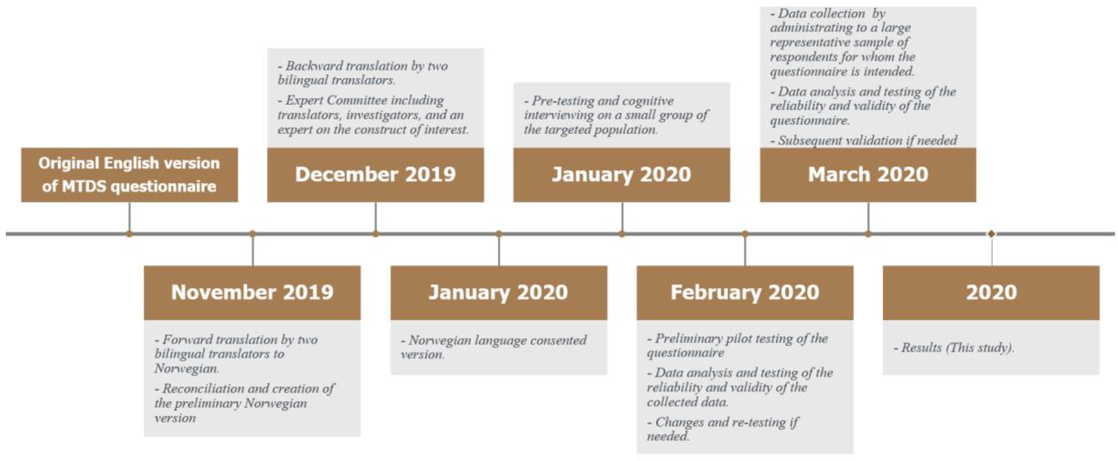
2.4. Procedures
Translation of the MTDS from English to Norwegian
2.5. Data Collection
2.6. Statistical Analysis
3. Results
3.1. Item Analysis of MTDS-N
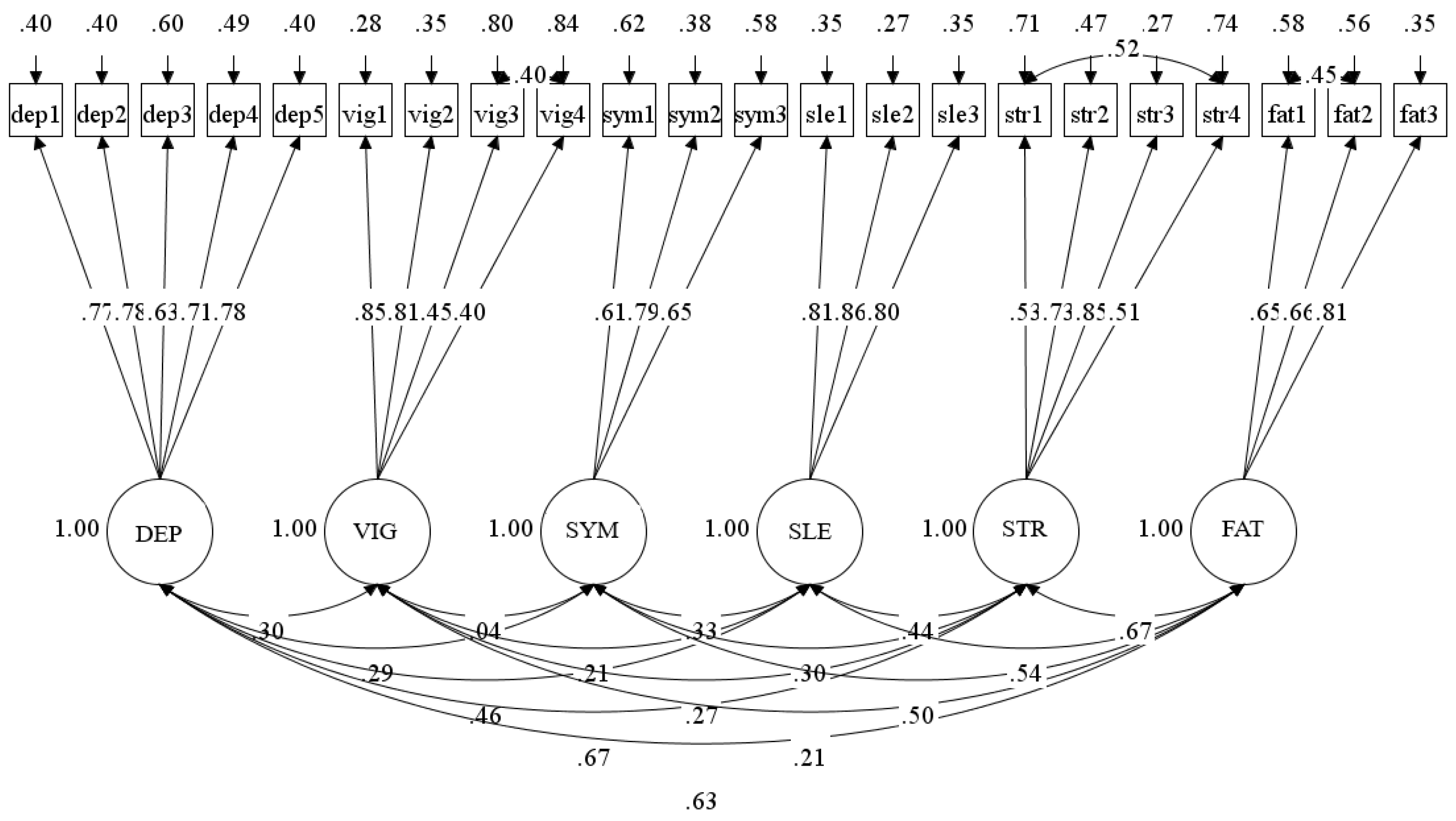
3.2. Confirmatory Factor Analysis
= (1035.880 − 604.085)(204 − 191)/[204 × 1.169) − (191 × 1.155)]
= 314.02
Scale Reliability
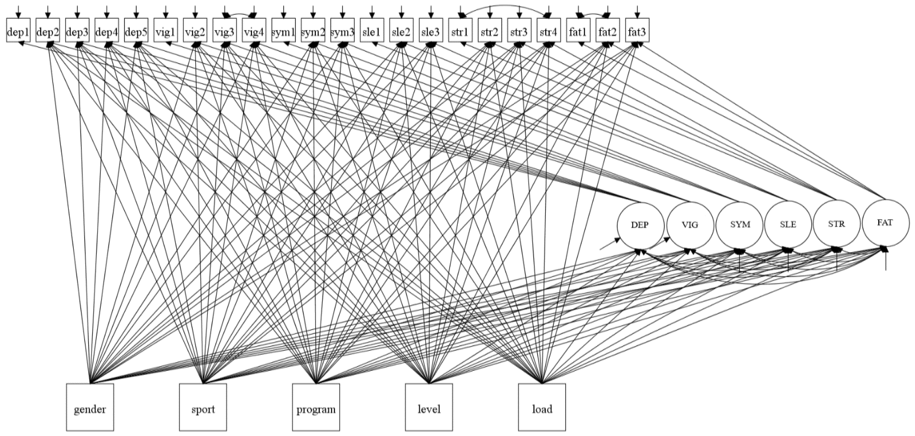
3.3. Estimating Group Differences in Latent Variables
3.4. Estimating Group Differences in Factor Indicators
4. Discussion
4.1. Confirmatory Factor Analysis
Scale Reliability
4.2. Estimating Group Differences in Latent Variables
4.3. Estimating Group Differences in Factor Indicators
5. Conclusions
Supplementary Materials
Author Contributions
Funding
Acknowledgments
Conflicts of Interest
References
- Stambulova, N.B.; Engström, C.; Franck, A.; Linnér, L.; Lindahl, K. Searching for an optimal balance: Dual career experiences of Swedish adolescent athletes. Psychol. Sport Exerc. 2015, 21, 4–14. [Google Scholar] [CrossRef]
- Kristiansen, E. Walking the line: How young athletes balance academic studies and sport in international competition. Sport Soc. 2017, 20, 47–65. [Google Scholar] [CrossRef] [Green Version]
- Christensen, M.K.; Sørensen, J.K. Sport or school? Dreams and dilemmas for talented young Danish football players. Eur. Phys. Educ. Rev. 2009, 15, 115–133. [Google Scholar] [CrossRef] [Green Version]
- Hamlin, M.J.; Wilkes, D.; Elliot, C.A.; Lizamore, C.A.; Kathiravel, Y. Monitoring training loads and perceived stress in young elite university athletes. Front. Physiol. 2019, 10, 34. [Google Scholar] [CrossRef] [PubMed] [Green Version]
- McKay, C.D.; Cumming, S.P.; Blake, T.J.B.P.; Rheumatology, R.C. Youth sport: Friend or Foe? Best Pract. Res. Clin. Rheumatol. 2019, 33, 141–157. [Google Scholar] [CrossRef] [PubMed]
- Jones, C.M.; Griffiths, P.C.; Mellalieu, S.D. Training load and fatigue marker associations with injury and illness: A systematic review of longitudinal studies. Sports Med. 2017, 47, 943–974. [Google Scholar] [CrossRef] [Green Version]
- Eckard, T.G.; Padua, D.A.; Hearn, D.W.; Pexa, B.S.; Frank, B.S. The relationship between training load and injury in athletes: A systematic review. Sports Med. 2018, 48, 1929–1961. [Google Scholar] [CrossRef]
- Kellmann, M.; Bertollo, M.; Bosquet, L.; Brink, M.; Coutts, A.J.; Duffield, R.; Erlacher, D.; Halson, S.L.; Hecksteden, A.; Heidari, J.; et al. Recovery and Performance in Sport: Consensus Statement. Int. J. Sports Physiol. Perform. 2018, 13, 240–245. [Google Scholar] [CrossRef] [Green Version]
- Meeusen, R.; Duclos, M.; Gleeson, M.; Rietjens, G.; Steinacker, J.; Urhausen, A. Prevention, diagnosis and treatment of the overtraining syndrome: ECSS position statement ‘task force’. Eur. J. Sport Sci. 2006, 6, 1–14. [Google Scholar] [CrossRef]
- Takarada, Y. Evaluation of muscle damage after a rugby match with special reference to tackle plays. Br. J. Sports Med. 2003, 37, 416–419. [Google Scholar] [CrossRef] [Green Version]
- McLellan, C.P.; Lovell, D.I.; Gass, G.C. Biochemical and endocrine responses to impact and collision during elite Rugby League match play. J. Strength Cond. Res. 2011, 25, 1553–1562. [Google Scholar] [CrossRef] [PubMed]
- Cunniffe, B.; Hore, A.J.; Whitcombe, D.M.; Jones, K.P.; Baker, J.S.; Davies, B. Time course of changes in immuneoendocrine markers following an international rugby game. Eur. J. Appl. Physiol. 2010, 108, 113–122. [Google Scholar] [CrossRef] [PubMed]
- McLellan, C.P.; Lovell, D.I.; Gass, G.C. Creatine kinase and endocrine responses of elite players pre, during, and post rugby league match play. J. Strength Cond. Res. 2010, 24, 2908–2919. [Google Scholar] [CrossRef] [PubMed] [Green Version]
- West, D.J.; Finn, C.V.; Cunningham, D.J.; Shearer, D.A.; Jones, M.R.; Harrington, B.J.; Crewther, B.T.; Cook, C.J.; Kilduff, L.P. Neuromuscular function, hormonal, and mood responses to a professional rugby union match. J. Strength Cond. Res. 2014, 28, 194–200. [Google Scholar] [CrossRef]
- Gill, N.D.; Beaven, C.M.; Cook, C. Effectiveness of post-match recovery strategies in rugby players. Br. J. Sports Med. 2006, 40, 260–263. [Google Scholar] [CrossRef] [Green Version]
- Soligard, T.; Schwellnus, M.; Alonso, J.-M.; Bahr, R.; Clarsen, B.; Dijkstra, H.P.; Gabbett, T.; Gleeson, M.; Hägglund, M.; Hutchinson, M.R. How much is too much?(Part 1) International Olympic Committee consensus statement on load in sport and risk of injury. Br. J. Sports Med. 2016, 50, 1030–1041. [Google Scholar] [CrossRef] [Green Version]
- Chiu, L.Z.F.; Barnes, J.L. The Fitness-Fatigue Model Revisited: Implications for Planning Short- and Long-Term Training. Strength Cond. J. 2003, 25, 42–51. [Google Scholar] [CrossRef]
- Matos, N.F.; Winsley, R.J.; Williams, C.A. Prevalence of nonfunctional overreaching/overtraining in young English athletes. Med. Sci. Sports Exerc. 2011, 43, 1287–1294. [Google Scholar] [CrossRef] [Green Version]
- Bourdon, P.C.; Cardinale, M.; Murray, A.; Gastin, P.; Kellmann, M.; Varley, M.C.; Gabbett, T.J.; Coutts, A.J.; Burgess, D.J.; Gregson, W. Monitoring athlete training loads: Consensus statement. Int. J. Sports Physiol. Perform. 2017, 12, S2–S161. [Google Scholar] [CrossRef]
- Saw, A.E.; Kellmann, M.; Main, L.C.; Gastin, P.B. Athlete self-report measures in research and practice: Considerations for the discerning reader and fastidious practitioner. Int. J. Sports Physiol. Perform. 2017, 12, S2–S127. [Google Scholar] [CrossRef]
- Borg, G.A. Psychophysical bases of perceived exertion. Med. Sci. Sports Exerc. 1982, 14, 377–381. [Google Scholar] [CrossRef] [PubMed]
- Calvert, T.W.; Banister, E.W.; Savage, M.V.; Bach, T. A systems model of the effects of training on physical performance. IEEE Trans. Syst. ManCybern. 1976, 94–102. [Google Scholar] [CrossRef]
- Foster, C. Monitoring training in athletes with reference to overtraining syndrome. Med. Sci. Sports Exerc. 1998, 30, 1164–1168. [Google Scholar] [CrossRef] [PubMed]
- Foster, C.; Florhaug, J.A.; Franklin, J.; Gottschall, L.; Hrovatin, L.A.; Parker, S.; Doleshal, P.; Dodge, C. A new approach to monitoring exercise training. J. Strength Cond. Res. 2001, 15, 109–115. [Google Scholar]
- Taylor, K.; Chapman, D.; Cronin, J.; Newton, M.J.; Gill, N. Fatigue monitoring in high performance sport: A survey of current trends. J. Aust. Strength. Cond. 2012, 20, 12–23. [Google Scholar]
- Windt, J.; Taylor, D.; Nabhan, D.; Zumbo, B.D. What is unified validity theory and how might it contribute to research and practice with athlete self-report measures. Br. J. Sports Med. 2019, 53, 1203–1204. [Google Scholar] [CrossRef]
- Jeffreys, I. A System for Monitoring Training Stress and Recovery in High School Athletes. Strength Cond. J. 2004, 26, 28–33. [Google Scholar] [CrossRef]
- Saw, A.E.; Main, L.C.; Gastin, P.B. Monitoring the athlete training response: Subjective self-reported measures trump commonly used objective measures: A systematic review. Br. J. Sports Med. 2016, 50, 281–291. [Google Scholar] [CrossRef]
- Main, L.; Grove, J.R. A multi-component assessment model for monitoring training distress among athletes. Eur. J. Sport Sci. 2009, 9, 195–202. [Google Scholar] [CrossRef] [Green Version]
- Main, L.C.; Warmington, S.A.; Korn, E.; Gastin, P.B. Utility of the multi-component training distress scale to monitor swimmers during periods of training overload. Res. Sports Med. 2016, 24, 254–265. [Google Scholar] [CrossRef]
- Woods, A.L.; Garvican-Lewis, L.A.; Lundy, B.; Rice, A.J.; Thompson, K.G. New approaches to determine fatigue in elite athletes during intensified training: Resting metabolic rate and pacing profile. PLoS ONE 2017, 12, e0173807. [Google Scholar] [CrossRef] [PubMed]
- Agwuenu, I.C.; Bettencourt, H.A.; Van Ness, J.M.; Jensen, C.D. Multicomponent training distress scale (MTDS) questionnaire to detect training distress in collegiate soccer players. Med. Sci. Sports Exerc. 2017, 49, 579. [Google Scholar] [CrossRef]
- Hofacker, M.L. Changes in Nutritional Biomarkers, Sleep, Perceived Stress, and Performance in Division I Female Soccer Players throughout a Competitive Season; Rutgers University-School of Graduate Studies: New Brunswick, NJ, USA, 2019. [Google Scholar]
- Woods, A.L.; Rice, A.J.; Garvican-Lewis, L.A.; Wallett, A.M.; Lundy, B.; Rogers, M.A.; Welvaert, M.; Halson, S.; McKune, A.; Thompson, K.G. The effects of intensified training on resting metabolic rate (RMR), body composition and performance in trained cyclists. PLoS ONE 2018, 13, e0191644. [Google Scholar] [CrossRef] [PubMed]
- Davis, P.; Halvarsson, A.; Lundström, W.; Lundqvist, C. Alpine ski coaches’ and athletes’ perceptions of factors influencing adaptation to stress in the classroom and on the slopes. Front. Psychol. 2019, 10, 1641. [Google Scholar] [CrossRef] [Green Version]
- Gescheit, D.T.; Cormack, S.J.; Reid, M.; Duffield, R. Consecutive days of prolonged tennis match play: Performance, physical, and perceptual responses in trained players. Int. J. Sports Physiol. Perform. 2015, 10, 913–920. [Google Scholar] [CrossRef] [PubMed]
- Nässi, A.; Ferrauti, A.; Meyer, T.; Pfeiffer, M.; Kellmann, M. Psychological tools used for monitoring training responses of athletes. Perform. Enhanc. Health 2017, 5, 125–133. [Google Scholar] [CrossRef]
- Kretzschmar, A.; Gignac, G.E. At what sample size do latent variable correlations stabilize? J. Res. Personal. 2019, 80, 17–22. [Google Scholar] [CrossRef] [Green Version]
- Schönbrodt, F.D.; Perugini, M. At what sample size do correlations stabilize? J. Res. Personal. 2013, 47, 609–612. [Google Scholar] [CrossRef] [Green Version]
- Hirschfeld, G.; Brachel, R.V.; Thielsch, M. Selecting items for Big Five questionnaires: At what sample size do factor loadings stabilize? J. Res. Personal. 2014, 53, 54–63. [Google Scholar] [CrossRef]
- Cohen, J. Statistical Power Analysis for the Behavioral Sciences; Routledge: New York, NY, USA, 1988. [Google Scholar]
- Cohen, S.; Kamarck, T.; Mermelstein, R. A global measure of perceived stress. J. Health Soc. Behav. 1983, 24, 385–396. [Google Scholar] [CrossRef]
- Terry, P.C.; Lane, A.M.; Fogarty, G.J. Construct validity of the Profile of Mood States—Adolescents for use with adults. Psychol. Sport Exerc. 2003, 4, 125–139. [Google Scholar] [CrossRef] [Green Version]
- Fry, R.; Grove, J.; Morton, A.; Zeroni, P.; Gaudieri, S.; Keast, D. Psychological and immunological correlates of acute overtraining. Br. J. Sports Med. 1994, 28, 241–246. [Google Scholar] [CrossRef] [Green Version]
- Raedeke, T.D.; Smith, A.L. Development and Preliminary Validation of an Athlete Burnout Measure. J. Sport Exerc. Psychol. 2001, 23, 281–306. [Google Scholar] [CrossRef]
- Guillemin, F.; Bombardier, C.; Beaton, D. Cross-cultural adaptation of health-related quality of life measures: Literature review and proposed guidelines. J. Clin. Epidemiol. 1993, 46, 1417–1432. [Google Scholar] [CrossRef]
- International Test Commission. The ITC Guidelines for Translating and Adapting Tests (Second edition). Int. J. Test. 2017, 18, 101–134. [Google Scholar]
- Guillemin, F.; Briancon, S.; Pourel, J. Validity and discriminant ability of a French version of the Health Assessment Questionnaire in early RA. Disabil Rehabil 1992, 14, 7. [Google Scholar]
- Leadingsystem. SurveyXact. Available online: http://www.surveyxact.com/about-us (accessed on 24 September 2020).
- Muthén, L.K.; Muthén, B. (1998–2017) Mplus User’s Guide, 8th ed.; Muthén & Muthén: Los Angeles, CA, USA, 2017. [Google Scholar]
- George, D.; Mallery, P. SPSS for Windows Step by Step: A Simple Guide and Reference, 11.0 Update, 4th ed.; Allyn and Bacon: Boston, MA, USA, 2003. [Google Scholar]
- Wang, J.; Wang, X. Structural Equation Modeling: Applicatins Using Mplus, 2nd ed.; Wiley & Sons Ltd.: Hoboken, NJ, USA, 2020. [Google Scholar]
- Field, A. Discovering Statistics Using IBM SPSS Statistics: And Sex and Drugs and Rock ’n’ Roll, 4th ed.; SAGE: Los Angeles, CA, USA, 2013. [Google Scholar]
- Schumacker, R.E.; Lomax, R.G. A Beginner’s Guide to Structural Equation Modeling, 2nd ed.; Lawrence Erlbaum Associates: Mahwah, NJ, USA, 2004. [Google Scholar]
- Hu, L.-T.; Bentler, P.M. Cutoff criteria for fit indexes in covariance structure analysis: Conventional criteria versus new alternatives. Struct. Equ. Model. 1999, 6, 1–55. [Google Scholar] [CrossRef]
- Steiger, J.H. Understanding the limitations of global fit assessment in structural equation modeling. Pers. Individ. Differ. 2007, 42, 893–898. [Google Scholar] [CrossRef]
- Hooper, D.; Coughlan, J.; Mullen, M.R. Structural equation modelling: Guidelines for determining model fit. Electron. J. Bus. Res. Methods 2008, 6, 53–60. [Google Scholar]
- Yu, C.-Y. Evaluating Cutoff Criteria of Model Fit Indices for Latent Variable Models with Binary and Continuous Outcomes; University of California: Los Angeles, CA, USA, 2002; Volume 30. [Google Scholar]
- Harrington, D. Confirmatory Factor Analysis; Oxford University Press: Oxford, UK, 2009. [Google Scholar]
- Brown, T.A. Confirmatory Factor Analysis for Apllied Research; The Guildford Press: New York, NY, USA, 2006. [Google Scholar]
- Mplus. Chi-Square Difference Testing Using the Satorra-Bentler Scaled Chi-Square. Available online: https://www.statmodel.com/chidiff.shtml (accessed on 14 October 2020).
- Funder, D.C.; Ozer, D.J. Evaluating effect size in psychological research: Sense and nonsense. Adv. Methods Pract. Psychol. Sci. 2019, 2, 156–168. [Google Scholar] [CrossRef]
- Raykov, T. Bias of coefficient afor fixed congeneric measures with correlated errors. Appl. Psychol. Meas. 2001, 25, 69–76. [Google Scholar] [CrossRef]
- Hayes, A.F.; Coutts, J.J. Use omega rather than Cronbach’s alpha for estimating reliability. But…. Commun. Methods Meas. 2020, 14, 1–24. [Google Scholar] [CrossRef]
- McNeish, D. Thanks coefficient alpha, we’ll take it from here. Psychol. Methods 2018, 23, 412. [Google Scholar] [CrossRef]
- Peters, G.-J.Y. The Alpha and the Omega of Scale Reliability and Validity: Why and how to Abandon Cronbach’s alpha and the route towards more comprehensive assessment of scale quality. Eur. Health Psychol. 2014, 16, 56–69. [Google Scholar]
- Dunn, T.J.; Baguley, T.; Brunsden, V. From alpha to omega: A practical solution to the pervasive problem of internal consistency estimation. Br. J. Psychol. 2014, 105, 399–412. [Google Scholar] [CrossRef] [PubMed] [Green Version]
- Lance, C.E.; Butts, M.M.; Michels, L.C. The Sources of Four Commonly Reported Cutoff Criteria:What Did They Really Say? Organ. Res. Methods 2006, 9, 202–220. [Google Scholar] [CrossRef]
- Taber, K.S. The Use of Cronbach’s Alpha When Developing and Reporting Research Instruments in Science Education. Res. Sci. Educ. 2018, 48, 1273–1296. [Google Scholar] [CrossRef]
- Streiner, D.L. Starting at the beginning: An introduction to coefficient alpha and internal consistency. J Pers Assess 2003, 80, 99–103. [Google Scholar] [CrossRef]
- Kaplan, D. Structural Equation Modeling: Foundations and Extensions, 2nd ed.; SAGE: Los Angeles, CA, USA, 2009; Volume 10. [Google Scholar]
- Jöreskog, K.G.; Goldberger, A.S. Estimation of a model with multiple indicators and multiple causes of a single latent variable. J. Am. Stat. Assoc. 1975, 70, 631–639. [Google Scholar]
- Muthén, B.O. Latent variable modeling in heterogeneous populations. Psychometrika 1989, 54, 557–585. [Google Scholar] [CrossRef]
- Woods, C.M. Evaluation of MIMIC-model methods for DIF testing with comparison to two-group analysis. Multivar. Behav. Res. 2009, 44, 1–27. [Google Scholar] [CrossRef]
- Woods, C.M.; Oltmanns, T.F.; Turkheimer, E. Illustration of MIMIC-model DIF testing with the schedule for nonadaptive and adaptive personality. J. Psychopathol. Behav. Assess. 2009, 31, 320. [Google Scholar] [CrossRef] [PubMed] [Green Version]
- Chernoff, H. Large-Sample Theory: Parametric Case. Ann. Math. Stat. 1956, 27, 1–22. [Google Scholar] [CrossRef]
- Lehmann, E.L. Elements of Large-Sample Theory; Springer: New York, NY, USA, 1956. [Google Scholar] [CrossRef]
- Miles, D.A. Risk Factors and Business Models: Understanding the Five Forces of Entrpreneurial Risk and the Causes of Business Failure. In Risk Factors and Business Models; Dissertation.com: Boca Raton, FL, USA, 2010. [Google Scholar]
- McQueen, A.; Tiro, J.A.; Vernon, S.W. Construct validity and invariance of four factors associated with colorectal cancer screening across gender, race, and prior screening. Cancer Epidemiol. Prev. Biomark. 2008, 17, 2231–2237. [Google Scholar] [CrossRef] [Green Version]
- Zhang, C.-Q.; Si, G.; Chung, P.-K.; Du, M.; Terry, P.C. Psychometric properties of the Brunel Mood Scale in Chinese adolescents and adults. J. Sports Sci. 2014, 32, 1465–1476. [Google Scholar] [CrossRef] [PubMed]
- Lan, M.F.; Lane, A.M.; Roy, J.; Hanin, N.A. Validity of the Brunel Mood Scale for use with Malaysian athletes. J. Sports Sci. Med. 2012, 11, 131. [Google Scholar]
- Cañadas, E.; García, C.M.; Sanchis, C.; Fargueta, M.; Herráiz, E.B. Spanish Validation of BRUMS in Sporting and Non-Sporting Populations. Eur. J. Hum. Mov. 2017, 38, 105–117. [Google Scholar]
- Puffer, J.C.; McShane, J.M. Depression and chronic fatigue in athletes. Clin. Sports Med. 1992, 11, 327–338. [Google Scholar] [CrossRef]
- Knight, S.; Harvey, A.; Towns, S.; Payne, D.; Lubitz, L.; Rowe, K.; Reveley, C.; Hennel, S.; Hiscock, H.; Scheinberg, A. How is paediatric chronic fatigue syndrome/myalgic encephalomyelitis diagnosed and managed by paediatricians? An Australian Paediatric Research Network Study. J. Paediatr. Child. Health 2014, 50, 1000–1007. [Google Scholar] [CrossRef]
- Boolani, A.; Manierre, M. An exploratory multivariate study examining correlates of trait mental and physical fatigue and energy. Fatigue Biomed. Health Behav. 2019, 7, 29–40. [Google Scholar] [CrossRef]
- Nixdorf, I.; Frank, R.; Hautzinger, M.; Beckmann, J. Prevalence of depressive symptoms and correlating variables among German elite athletes. J. Clin. Sport Psychol. 2013, 7, 313–326. [Google Scholar] [CrossRef]
- Hammen, C.; Kim, E.Y.; Eberhart, N.K.; Brennan, P.A. Chronic and acute stress and the prediction of major depression in women. Depress Anxiety 2009, 26, 718–723. [Google Scholar] [CrossRef] [PubMed] [Green Version]
- De Francisco, C.; Arce, C.; Vílchez, M.d.P.; Vales, Á. Antecedents and consequences of burnout in athletes: Perceived stress and depression. Int. J. Clin. Health Psychol. 2016, 16, 239–246. [Google Scholar] [CrossRef] [PubMed]
- Kask, A.; Svanberg, K. Mental Health among Swedish Elite Athletes: Depression, Overtraining, Help Seeking, and Stigma; Umeå Univeristy: Umeå, Sweden, 2017. [Google Scholar]
- Bettencourt, H.A. Does Heart Rate Recovery Detect Training Distress in Collegiate Soccer Players? University of the Pacific: Stockton, CA, USA, 2016. [Google Scholar]
- Gitchel, W.D.; Roessler, R.T.; Turner, R.C. Gender effect according to item directionality on the perceived stress scale for adults with multiple sclerosis. Rehabil. Couns. Bull. 2011, 55, 20–28. [Google Scholar] [CrossRef]
- Gerber, M.; Best, S.; Meerstetter, F.; Walter, M.; Ludyga, S.; Brand, S.; Bianchi, R.; Madigan, D.J.; Isoard-Gautheur, S.; Gustafsson, H. Effects of stress and mental toughness on burnout and depressive symptoms: A prospective study with young elite athletes. J. Sci. Med. Sport 2018, 21, 1200–1205. [Google Scholar] [CrossRef] [PubMed]
- Wu, A.D.; Zhen, L.; Zumbo, B.D. Decoding the meaning of factorial invariance and updating the practice of multi-group confirmatory factor analysis: A demonstration with TIMSS data. Pract. Assess. Res. Eval. 2007, 12, 3. [Google Scholar]
- Carle, A.C.; Millsap, R.E.; Cole, D.A. Measurement bias across gender on the Children’s Depression Inventory: Evidence for invariance from two latent variable models. Educ. Psychol. Meas. 2008, 68, 281–303. [Google Scholar] [CrossRef]
- Nolen-Hoeksema, S. Gender differences in depression. Am. Psychol. Soc. 2001, 10, 173–176. [Google Scholar] [CrossRef] [Green Version]
- Thayer, J.F.; Rossy, L.A.; Ruiz-Padial, E.; Johnsen, B.H. Gender differences in the relationship between emotional regulation and depressive symptoms. Cogn. Ther. Res. 2003, 27, 349–364. [Google Scholar] [CrossRef]
- Terry, P.C.; Malekshahi, M.; Delva, H.A. Development and initial validation of the Farsi Mood Scale. Int. J. Sport Exerc. Psychol. 2012, 10, 112–122. [Google Scholar] [CrossRef] [Green Version]
- Sigmon, S.T.; Pells, J.J.; Boulard, N.E.; Whitcomb-Smith, S.; Edenfield, T.M.; Hermann, B.A.; LaMattina, S.M.; Schartel, J.G.; Kubik, E. Gender differences in self-reports of depression: The response bias hypothesis revisited. Sex Roles 2005, 53, 401–411. [Google Scholar] [CrossRef]
- Brody, L.R.; Hall, J.A. Gender, emotion, and expression. In Handbook of Emotions, 2nd ed.; Lewis, M., Haviland-Jones, J.M., Eds.; Guilford Press: NewYork, NY, USA, 2000; pp. 338–349. [Google Scholar]
- Chevron, E.S.; Quinlan, D.M.; Blatt, S.J. Sex roles and gender differences in the experience of depression. J. Abnorm. Psychol. 1978, 87, 680–683. [Google Scholar] [CrossRef] [PubMed]
- Conway, M. On Sex Roles and Representations of Emotional Experience: Masculinity, Femininity, and Emotional Awareness. Sex Roles 2000, 43, 687–698. [Google Scholar] [CrossRef]
- Pluhar, E.; McCracken, C.; Griffith, K.L.; Christino, M.A.; Sugimoto, D.; Meehan, W.P., III. Team sport athletes may be less likely to suffer anxiety or depression than individual sport athletes. J. Sports Sci. Med. 2019, 18, 490. [Google Scholar]
- Nixdorf, I.; Frank, R.; Beckmann, J. Comparison of athletes’ proneness to depressive symptoms in individual and team sports: Research on psychological mediators in junior elite athletes. Front. Psychol. 2016, 7, 893. [Google Scholar] [CrossRef] [Green Version]
- Elbe, A.-M.; Nylandsted Jensen, S. Commentary: Comparison of athletes’ proneness to depressive symptoms in individual and team sports: Research on psychological mediators in junior elite athletes. Front. Psychol. 2016, 7, 1782. [Google Scholar] [CrossRef] [PubMed] [Green Version]
- Jewett, R.; Sabiston, C.M.; Ashdown-Franks, G.; Brunet, J.; Bélanger, M.; O’Loughlin, E.K.; O’Loughlin, J.L. Team versus individual sports participation in adolescence and depressive symptoms in early adulthood. J. Exerc. Mov. Sport Scapps Refereed Abstr. Repos. 2014, 46, 157. [Google Scholar]
- Birrer, D.; Lienhard, D.; Williams, C.A.; Röthlin, P.; Morgan, G. Prevalence of non-functional overreaching and the overtraining syndrome in Swiss elite athletes. Schweiz Z Sportmed. Sporttraumatol 2013, 61, 23–29. [Google Scholar]
- Houlihan, B.; Green, M. Comparative elite sport development. In Comparative Elite Sport Development: Systems, Structures and Public Policy; Houlihan, B., Green, M., Eds.; Elsevier: Oxford, UK, 2008; pp. 1–21. [Google Scholar]
- Houlihan, B. Mechanisms of international influence on domestic elite sport policy. Int. J. Sport Policy Politics 2009, 1, 51–69. [Google Scholar] [CrossRef] [Green Version]
- Skille, E.Å.; Chroni, S.A. Norwegian sports federations’ organizational culture and national team success. Int. J. Sport Policy Politics 2018, 10, 321–333. [Google Scholar] [CrossRef]
- Tavares, F.; Healey, P.; Smith, T.B.; Driller, M. The effect of training load on neuromuscular performance, muscle soreness and wellness during an in-season non-competitive week in elite rugby athletes. J. Sports Med. Phys. Fit. 2017, 58, 1565–1571. [Google Scholar] [CrossRef] [PubMed]
- Moalla, W.; Fessi, M.S.; Farhat, F.; Nouira, S.; Wong, D.P.; Dupont, G. Relationship between daily training load and psychometric status of professional soccer players. Res. Sports Med. 2016, 24, 387–394. [Google Scholar] [CrossRef]
- Gustafsson, H.; Holmberg, H.-C.; Hassmen, P. An elite endurance athlete’s recovery from underperformance aided by a multidisciplinary sport science support team. Eur. J. Sport Sci. 2008, 8, 267–276. [Google Scholar] [CrossRef]
- Droppleman, L.; Lorr, M.; McNair, D. Profile of Mood States (POMS)- Revised Manual; Educational and Industrial Testing Service: San Diego, CA, USA, 1992. [Google Scholar]
- Boolani, A.; O’Connor, P.J.; Reid, J.; Ma, S.; Mondal, S. Predictors of feelings of energy differ from predictors of fatigue. Fatigue: Biomed. Health Behav. 2019, 7, 12–28. [Google Scholar] [CrossRef]
- Groenvold, M.; Petersen, M.A. The role and use of differential item functioning (DIF) analysis of quality of life data from clinical trials. In Assessing Quality of Life in Clinical Trials, 2nd ed.; Fayers, P., Hays, R., Eds.; Oxford University Press: Oxford, NY, USA, 2005; pp. 195–208. [Google Scholar]
- Bartolucci, F.; Bacci, S.; Gnaldi, M. Statistical Analysis of Questionnaires: A Unified Approach Based on R and Stata; CRC Press: Broken Sound Parkway, FL, USA, 2016. [Google Scholar]
- Borsboom, D. When does measurement invariance matter? Med Care 2006, 44, S176–S181. [Google Scholar] [CrossRef] [PubMed] [Green Version]
- Rouquette, A.; Hardouin, J.B.; Vanhaesebrouck, A.; Sébille, V.; Coste, J. Differential Item Functioning (DIF) in composite health measurement scale: Recommendations for characterizing DIF with meaningful consequences within the Rasch model framework. PLoS ONE 2019, 14, e0215073. [Google Scholar] [CrossRef] [PubMed] [Green Version]
- Caputo, A. Social desirability bias in self-reported well-being measures: Evidence from an online survey. Univ. Psychol. 2017, 16, 245–255. [Google Scholar] [CrossRef] [Green Version]


| Characteristics (Total) 1 | Modalities | Frequency or M ± SD | % |
|---|---|---|---|
| Gender (630) | Male | 327 | 51.9 |
| Female | 303 | 48.1 | |
| Type of sport (630) | Individual | 207 | 32.9 |
| Team sport | 423 | 67.1 | |
| Region (632) | West Norway | 344 | 54.4 |
| East Norway | 148 | 23.4 | |
| Mid Norway | 160 | 16.8 | |
| Northern Norway | 34 | 5.4 | |
| Age in years (631) | Male | 17.37 ± 0.06 | |
| Female | 17.23 ± 0.05 | ||
| Training hours (617) | Total | 12.54 ± 4.99 | |
| Specialization in general studies | 12.60 ± 4.95 | ||
| Sports and physical education | 12.45 ± 5.06 | ||
| School program 2 (632) | Specialization in general studies | 369 | 58.4 |
| Sports and physical education | 263 | 41.6 | |
| School level 3 (632) | First grade | 232 | 36.7 |
| Second grade | 239 | 37.8 | |
| Third grade | 161 | 25.5 |
| Descriptive Statistics | |||||
|---|---|---|---|---|---|
| Type of Sport | Frequency | % | Type of Sport | Frequency | % |
| Soccer | 306 | 48.6 | Sailing | 6 | 1.0 |
| Handball | 91 | 14.4 | Martial art | 9 | 1.4 |
| Swimming | 24 | 3.8 | Badminton | 5 | 0.8 |
| Track field | 21 | 3.3 | Cheerleading | 1 | 0.2 |
| Gymnastics | 11 | 1.7 | Strength training | 4 | 0.6 |
| Ice hockey | 19 | 3.0 | Sky jumping | 1 | 0.2 |
| Cross-country skiing | 34 | 5.4 | Diving | 1 | 0.2 |
| Orienteering | 8 | 1.3 | Sports drill | 4 | 0.6 |
| Alpine skiing | 15 | 2.4 | Shooting | 1 | 0.2 |
| Cycling | 12 | 1.9 | Snowboard | 1 | 0.2 |
| Golf | 5 | 0.8 | Jet ski | 1 | 0.2 |
| Floorball | 2 | 0.3 | Dance | 1 | 0.2 |
| Volleyball | 5 | 0.8 | Motocross | 2 | 0.3 |
| Rowing | 3 | 0.5 | Triathlon | 2 | 0.3 |
| Biathlon | 12 | 1.9 | Freeski | 1 | 0.2 |
| Show jumping | 12 | 1.9 | Climbing | 1 | 0.2 |
| Ice skate | 4 | 0.6 | Figure skating | 1 | 0.2 |
| Tennis | 4 | 0.6 | |||
| Items | Descriptive Statistics | |||
|---|---|---|---|---|
| M | SD | Skewness | Kurtosis | |
| Depression (dep1–dep5) | ||||
| Miserable (dep1) | 1.47 | 0.82 | 1.95 | 3.44 |
| Unhappy (dep2) | 1.75 | 0.94 | 1.27 | 1.09 |
| Bitter (dep3) | 1.64 | 0.86 | 1.49 | 2.16 |
| Downhearted (dep4) | 2.03 | 1.06 | 0.92 | 0.11 |
| Depressed (dep5) | 1.49 | 0.90 | 2.09 | 3.97 |
| Vigor (vig1–vig4) | ||||
| Energetic (vig1) | 2.70 | 0.99 | 0.38 | −0.08 |
| Lively (vig2) | 2.61 | 0.95 | 0.54 | 0.03 |
| Active (vig3) | 2.52 | 0.90 | 0.32 | −0.24 |
| Alert (vig4) | 2.87 | 0.94 | 0.30 | −0.21 |
| Physical symptoms (sym1–sym3) | ||||
| Muscle soreness (sym1) | 2.52 | 1.03 | 0.18 | −0.68 |
| Heavy arms or legs (sym2) | 2.43 | 0.98 | 0.38 | −0.44 |
| Stiff/sore joints (sym3) | 2.11 | 1.03 | 0.73 | −0.19 |
| Sleep disturbances (sle1–sle3) | ||||
| Difficulties falling asleep (sle1) | 2.15 | 1.18 | 0.84 | −0.32 |
| Restless sleep (sle2) | 2.06 | 1.16 | 0.90 | −0.21 |
| Insomnia (sle3) | 1.83 | 1.11 | 1.22 | 0.51 |
| Stress (str1–str4) | ||||
| Stressed (str1) | 3.06 | 1.11 | −0.02 | −0.65 |
| Could not cope (str2) | 2.76 | 1.02 | 0.10 | −0.46 |
| Difficulties piling up (str3) | 2.12 | 0.96 | 0.68 | 0.08 |
| Nervous (str4) | 2.78 | 1.09 | 0.15 | −0.56 |
| Fatigue (fat1–fat3) | ||||
| Tired (fat1) | 2.69 | 0.98 | 0.28 | −0.42 |
| Sleepy (fat2) | 2.54 | 1.09 | 0.43 | −0.55 |
| Worn-out (fat3) | 2.46 | 1.07 | 0.41 | −0.59 |
| Fit Indices | The Hypothesized Model | The Alternative Model |
|---|---|---|
| χ2 | 814.824 | 523.017 |
| df | 194 | 191 |
| p | <0.001 | <0.001 |
| RMSEA | 0.071 | 0.052 |
| CI | 0.066–0.076 | 0.047–0.058 |
| CFI | 0.873 | 0.932 |
| TLI | 0.848 | 0.918 |
| SRMR | 0.057 | 0.050 |
| MLR | ML | |||
|---|---|---|---|---|
| Alternative model | ||||
| T1 523.017 | d1 191 | c1 1.155 | T1 × c1 604.085 | d1 191 |
| Restricted model | ||||
| T0 886.125 | d0 204 | c0 1.169 | T0 × c0 1035.880 | d0 204 |
| Item | Hypothesized | R2 | Alternative | R2 |
|---|---|---|---|---|
| Miserable (dep1) | 0.768 | 0.590 | 0.773 | 0.598 |
| Unhappy (dep2) | 0.782 | 0.611 | 0.777 | 0.604 |
| Bitter (dep3) | 0.632 | 0.400 | 0.631 | 0.399 |
| Downhearted (dep4) | 0.715 | 0.512 | 0.713 | 0.508 |
| Depressed (dep5) | 0.773 | 0.598 | 0.775 | 0.601 |
| Energetic (vig1) | 0.830 | 0.689 | 0.864 | 0.716 |
| Lively (vig2) | 0.798 | 0.637 | 0.805 | 0.648 |
| Active (vig3) | 0.498 | 0.248 | 0.451 | 0.204 |
| Alert (vig4) | 0.455 | 0.207 | 0.404 | 0.163 |
| Muscle soreness (sym1) | 0.614 | 0.377 | 0.613 | 0.376 |
| Heavy arms or legs (sym2) | 0.789 | 0.623 | 0.790 | 0.625 |
| Stiff/sore joints (sym3) | 0.650 | 0.423 | 0.650 | 0.422 |
| Difficulty falling asleep (sle1) | 0.803 | 0.645 | 0.805 | 0.649 |
| Restless sleep (sle2) | 0.855 | 0.732 | 0.856 | 0.732 |
| Insomnia (sle3) | 0.806 | 0.649 | 0.804 | 0.646 |
| Stressed (str1) | 0.627 | 0.393 | 0.534 | 0.285 |
| Could not cope (str2) | 0.699 | 0.489 | 0.726 | 0.527 |
| Difficulties piling up (str3) | 0.809 | 0.654 | 0.855 | 0.731 |
| Nervous (str4) | 0.601 | 0.361 | 0.507 | 0.257 |
| Tired (fat1) | 0.797 | 0.635 | 0.650 | 0.422 |
| Sleepy (fat2) | 0.809 | 0.655 | 0.664 | 0.440 |
| Worn-out (fat3) | 0.700 | 0.490 | 0.806 | 0.649 |
| Factor | Depression | Vigor | Physical Symptoms | Sleep Disturbances | Stress | Fatigue |
|---|---|---|---|---|---|---|
| DEP | 1 | 0.304 ** | 0.292 ** | 0.460 ** | 0.668 ** | 0.634 ** |
| VIG | −0.194 | 1 | 0.035 | 0.207 ** | 0.269 ** | 0.207 ** |
| SYM | −0.228 | 0.041 | 1 | 0.331 ** | 0.305 ** | 0.502 ** |
| SLE | −0.394 | 0.110 | 0.247 | 1 | 0.441 ** | 0.541 ** |
| STR | 0.437 | −0.259 | −0.181 | −0.273 | 1 | 0.667 ** |
| FAT | −0.208 | 0.182 | 0.321 | 0.207 | −0.311 | 1 |
| Factor | Estimate | Lower 5% CI | Upper 5% CI |
|---|---|---|---|
| Depression | 0.853 | 0.831 | 0.887 |
| Vigor | 0.747 | 0.714 | 0.799 |
| Physical symptoms | 0.725 | 0.690 | 0.779 |
| Sleep disturbances | 0.862 | 0.841 | 0.895 |
| Stress | 0.745 | 0.715 | 0.739 |
| Fatigue | 0.753 | 0.717 | 0.809 |
| Factor | Descriptive Statistics | |
|---|---|---|
| M | SD | |
| 1. Depression (dep) | 1.67 | 0.92 |
| 2. Vigor (vig) | 2.67 | 0.94 |
| 3. Physical symptoms (sym) | 2.35 | 1.01 |
| 4. Sleep disturbances (sle) | 2.01 | 1.15 |
| 5. Stress (str) | 2.68 | 1.05 |
| 6. Fatigue (fat) | 2.56 | 1.05 |
| Total score a | 13.96 | 6.11 |
| Factor (Explained Variances) | Covariates | β | S.E. | p |
|---|---|---|---|---|
| Depression (0.045 = 4.5%) | Gender | 0.269 | 0.086 | 0.002 * |
| Sport | −0.172 | 0.103 | 0.096 | |
| Training | −0.008 | 0.010 | 0.445 | |
| Program | 0.090 | 0.038 | 0.020 * | |
| Level | 0.149 | 0.057 | 0.008 * | |
| Vigor (0.094 = 9.4%) | Gender | 0.135 | 0.079 | 0.089 |
| Sport | −0.062 | 0.092 | 0.501 | |
| Training | −0.011 | 0.007 | 0.143 | |
| Program | −0.237 | 0.038 | 0.000 ** | |
| Level | 0.141 | 0.048 | 0.003 | |
| Physical symptoms (0.038 = 3.8%) | Gender | 0.213 | 0.093 | 0.022 * |
| Sport | 0.231 | 0.105 | 0.028 * | |
| Training | 0.024 | 0.010 | 0.020 * | |
| Program | 0.110 | 0.040 | 0.007 * | |
| Level | −0.008 | 0.061 | 0.895 | |
| Sleep disturbances (0.059 = 5.9%) | Gender | 0.448 | 0.086 | 0.000 ** |
| Sport | −0.090 | 0.100 | 0.370 | |
| Training | −0.012 | 0.008 | 0.163 | |
| Program | 0.044 | 0.034 | 0.193 | |
| Level | 0.073 | 0.055 | 0.186 | |
| Stress (0.080 = 8.0%) | Gender | 0.502 | 0.089 | 0.000 ** |
| Sport | −0.042 | 0.105 | 0.686 | |
| Training | −0.012 | 0.009 | 0.207 | |
| Program | 0.105 | 0.045 | 0.020 * | |
| Level | 0.079 | 0.056 | 0.159 | |
| Fatigue (0.031 = 3.1%) | Gender | 0.235 | 0.094 | 0.012 * |
| Sport | 0.048 | 0.106 | 0.650 | |
| Training | −.016 | 0.009 | 0.090 | |
| Program | 0.094 | 0.042 | 0.025 * | |
| Level | 0.066 | 0.064 | 0.306 |
| Indicators | Covariates | β | S.E. | p | Effect Size |
|---|---|---|---|---|---|
| dep2 (unhappy) | Gender | 0.255 | 0.072 | 0.000 ** | M |
| Program | −0.194 | 0.045 | 0.000 ** | S | |
| dep3 (bitter) | Sport | 0.164 | 0.072 | 0.023 * | S |
| dep4 (downhearted) | Gender | 0.287 | 0.075 | 0.000 ** | M |
| Program | −0.213 | 0.043 | 0.000 ** | M | |
| dep5 (depressed) | Gender | 0.182 | 0.064 | 0.004 * | S |
| vig2 (lively) | Program | 0.231 | 0.046 | 0.000 ** | M |
| vig3 (active) | Program | 0.143 | 0.033 | 0.000 ** | S |
| Load | −0.174 | 0.069 | 0.012 * | S | |
| vig4 (alert) | Load | −0.200 | 0.072 | 0.006 * | M |
| sle2 (restless sleep) | Gender | 0.181 | 0.075 | 0.016 * | S |
| str2 (cope) | Gender | −0.295 | 0.108 | 0.006 * | M |
| Program | 0.528 | 0.061 | 0.000 ** | VL | |
| str3 (piling) | Gender | −0.369 | 0.111 | 0.001 * | L |
| Program | 0.559 | 0.062 | 0.000 ** | VL | |
| str4 (nervous) | Program | 0.151 | 0.044 | 0.001 * | S |
| fat2 (sleepy) | Gender | −0.212 | 0.070 | 0.002 * | M |
| Level | −0.090 | 0.045 | 0.047 * | VS | |
| fat3 (worn-out) | Program | −0.107 | 0.047 | 0.017 * | S |
| Level | −0.177 | 0.060 | 0.003 * | S |
Publisher’s Note: MDPI stays neutral with regard to jurisdictional claims in published maps and institutional affiliations. |
© 2020 by the authors. Licensee MDPI, Basel, Switzerland. This article is an open access article distributed under the terms and conditions of the Creative Commons Attribution (CC BY) license (http://creativecommons.org/licenses/by/4.0/).
Share and Cite
Hagum, C.N.; Shalfawi, S.A.I. The Factorial Validity of the Norwegian Version of the Multicomponent Training Distress Scale (MTDS-N). Int. J. Environ. Res. Public Health 2020, 17, 7603. https://doi.org/10.3390/ijerph17207603
Hagum CN, Shalfawi SAI. The Factorial Validity of the Norwegian Version of the Multicomponent Training Distress Scale (MTDS-N). International Journal of Environmental Research and Public Health. 2020; 17(20):7603. https://doi.org/10.3390/ijerph17207603
Chicago/Turabian StyleHagum, Cathrine Nyhus, and Shaher A. I. Shalfawi. 2020. "The Factorial Validity of the Norwegian Version of the Multicomponent Training Distress Scale (MTDS-N)" International Journal of Environmental Research and Public Health 17, no. 20: 7603. https://doi.org/10.3390/ijerph17207603