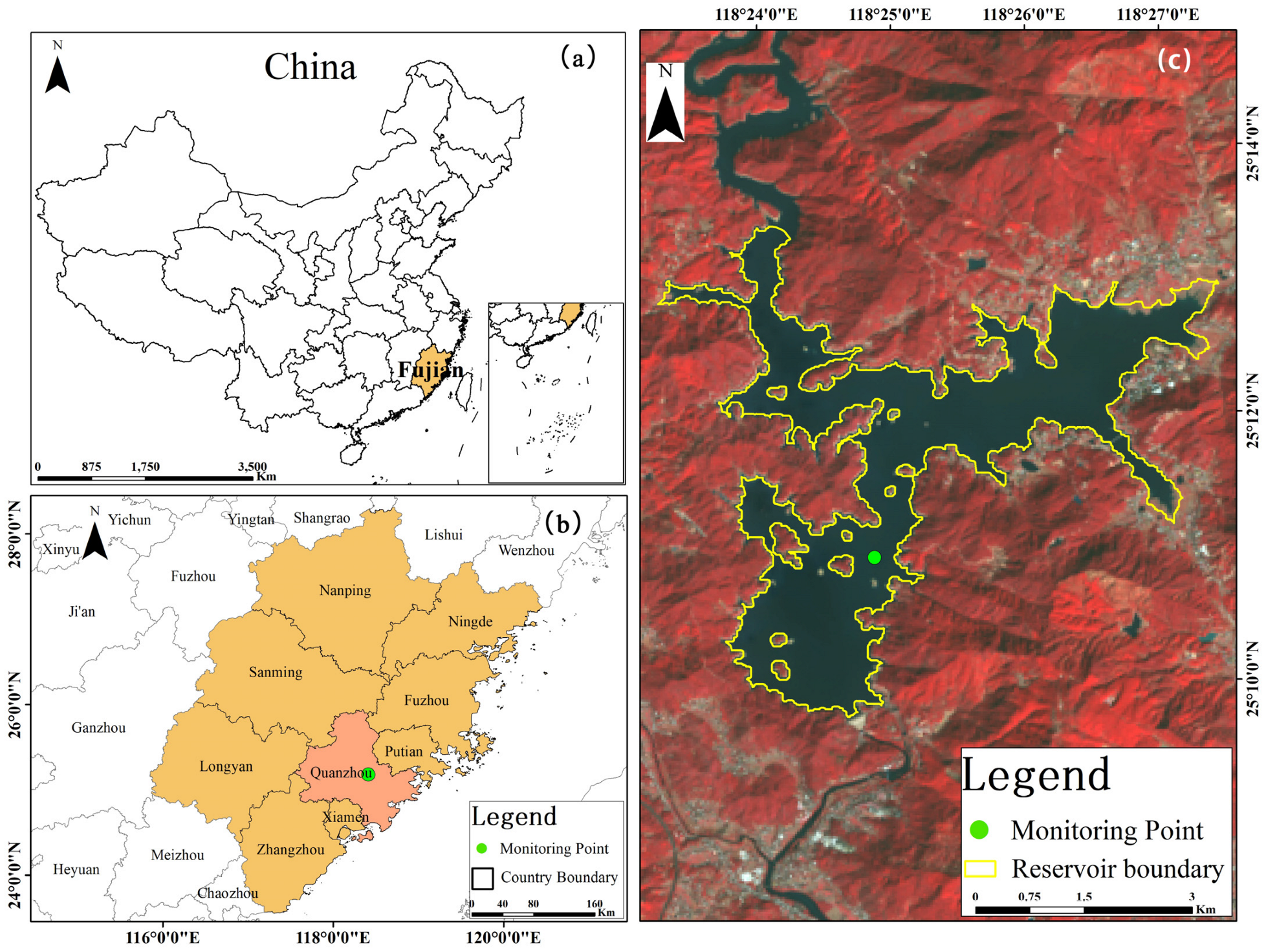
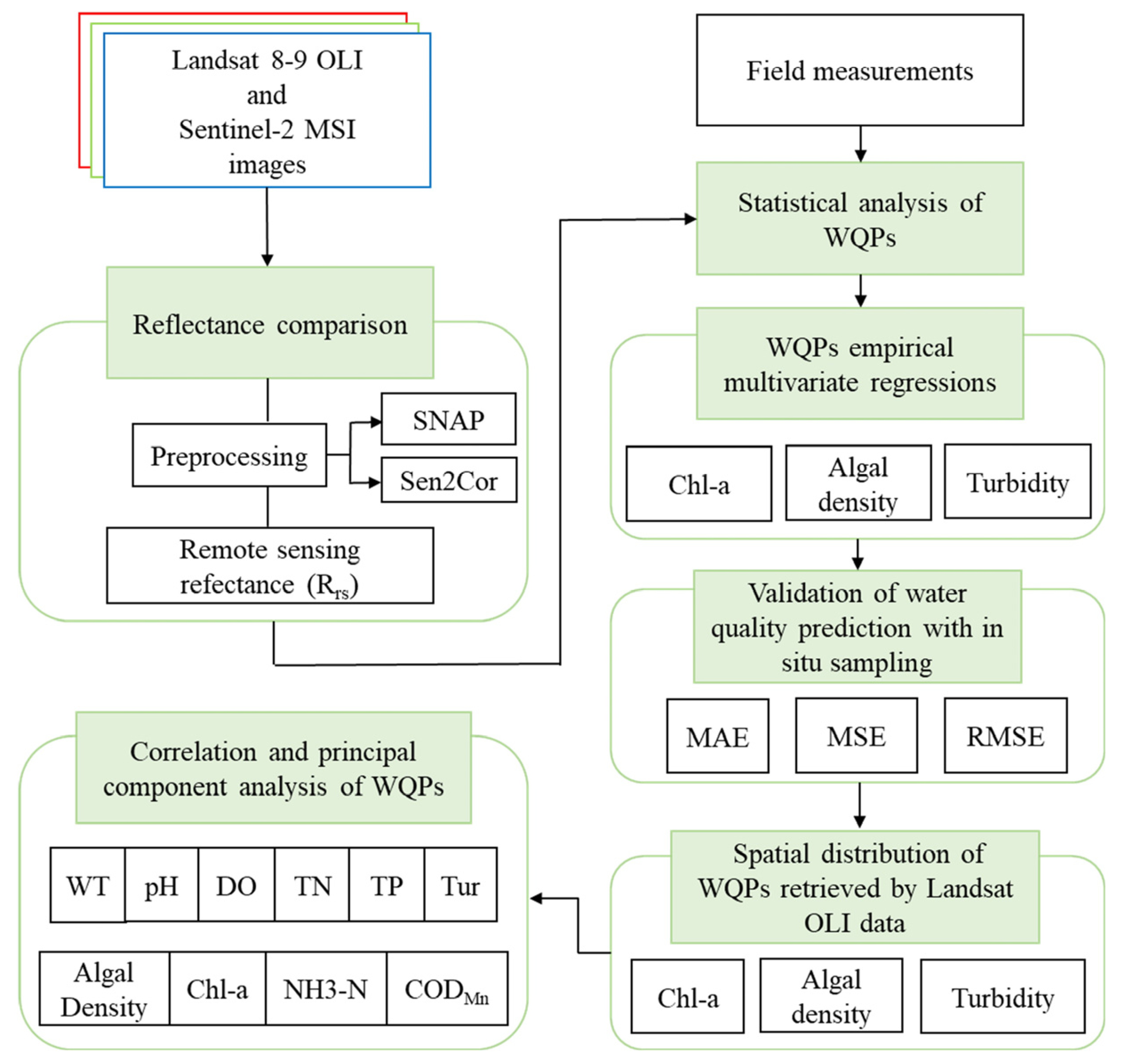
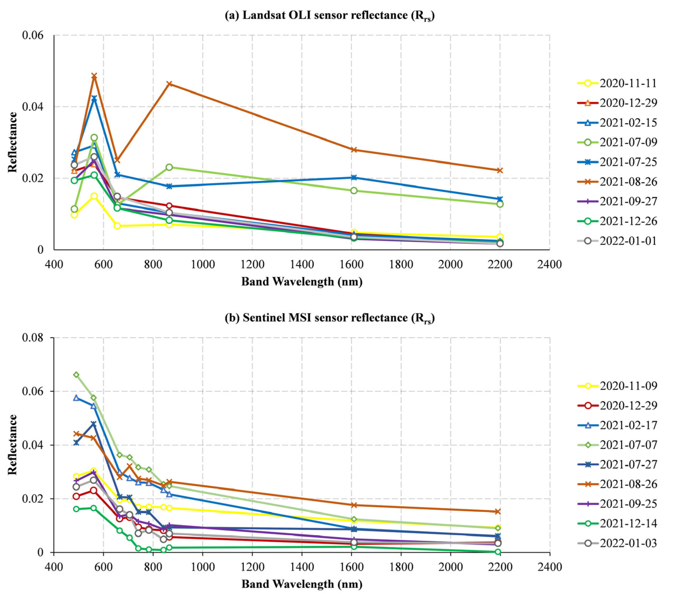
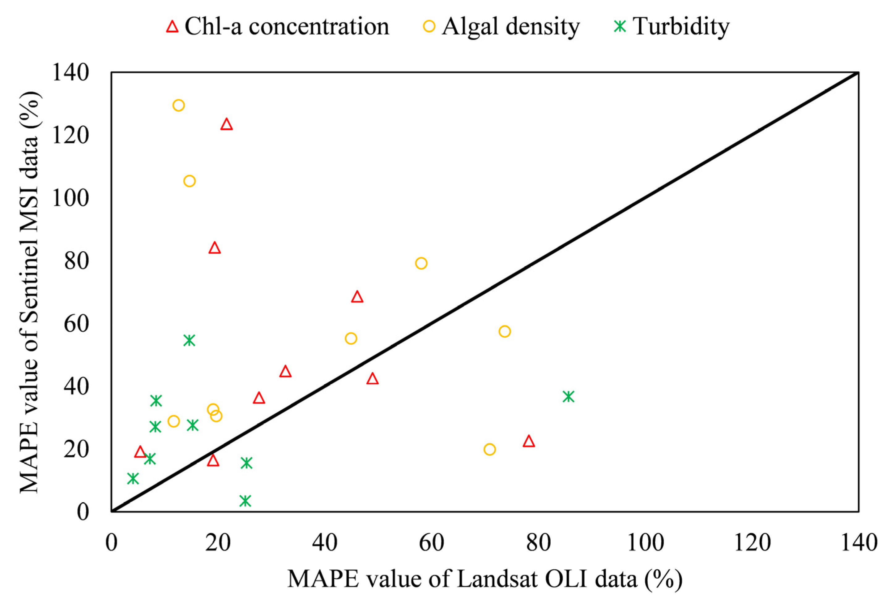
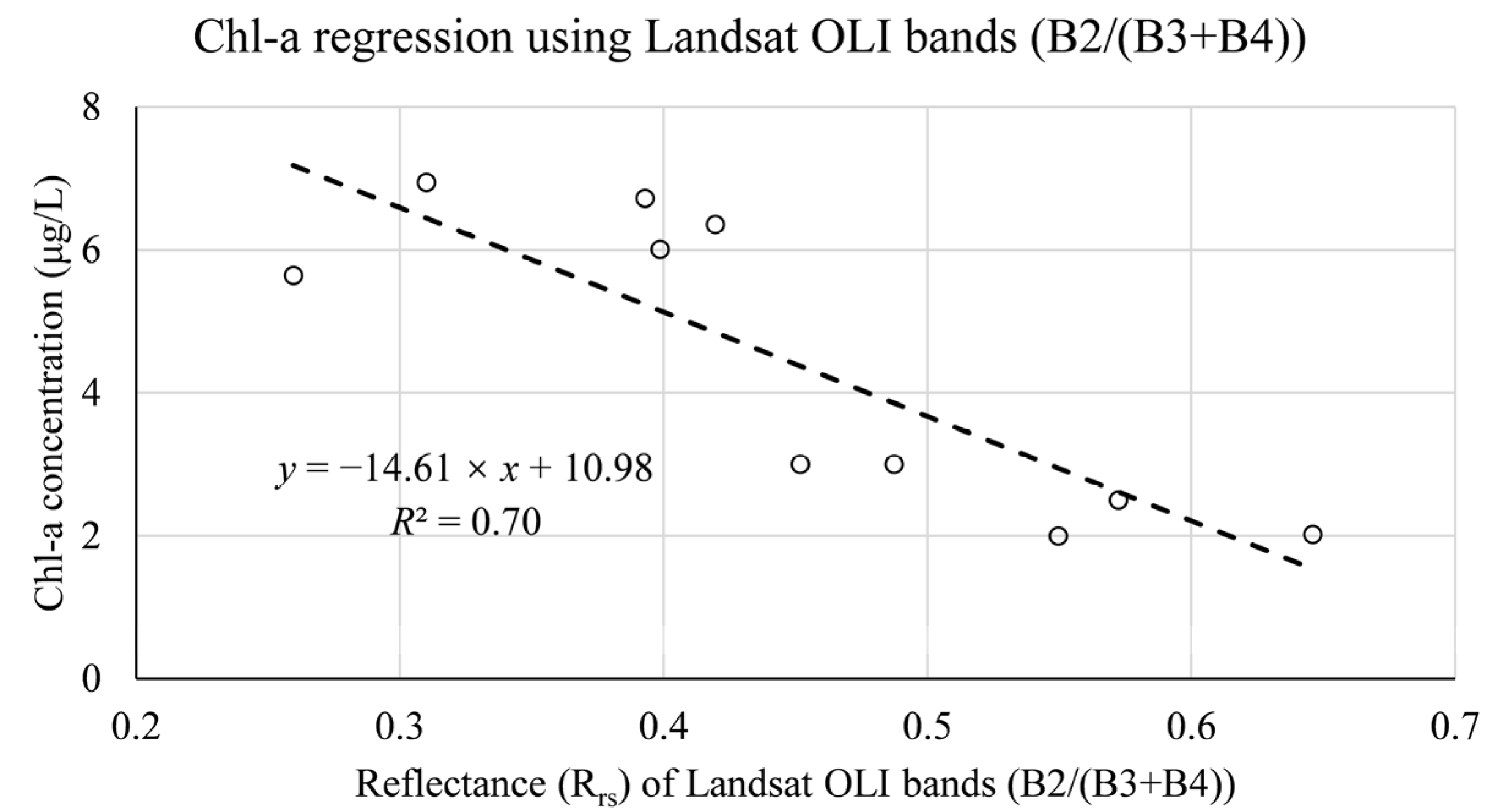
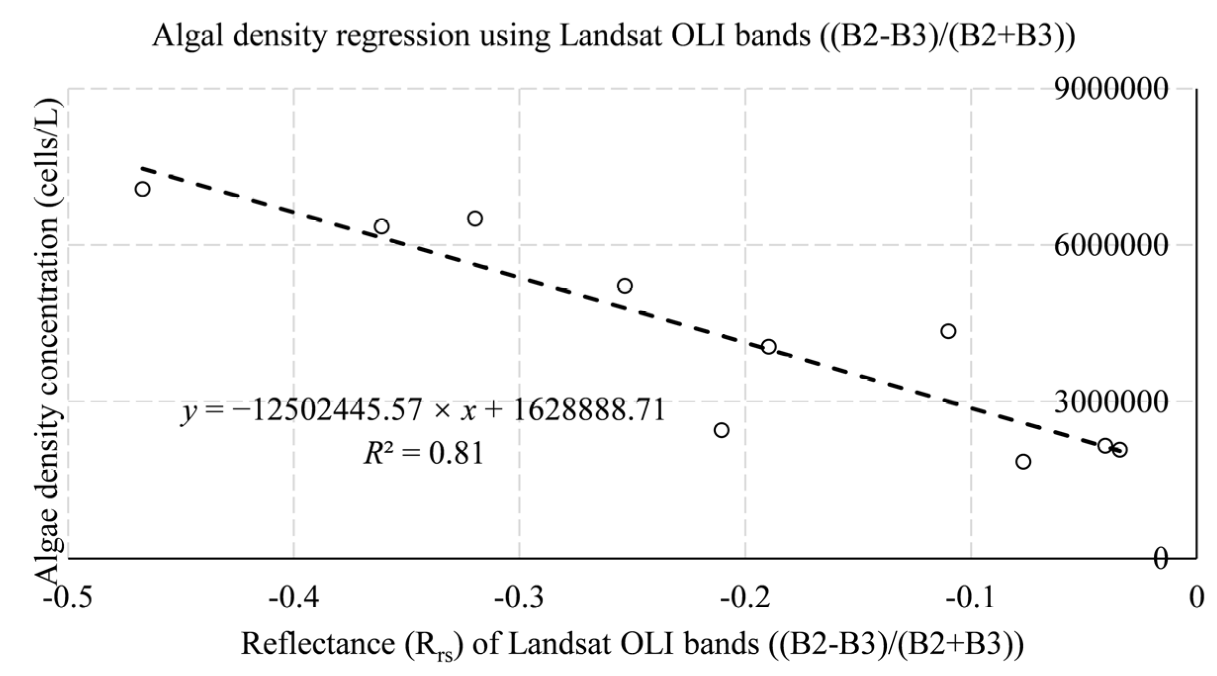
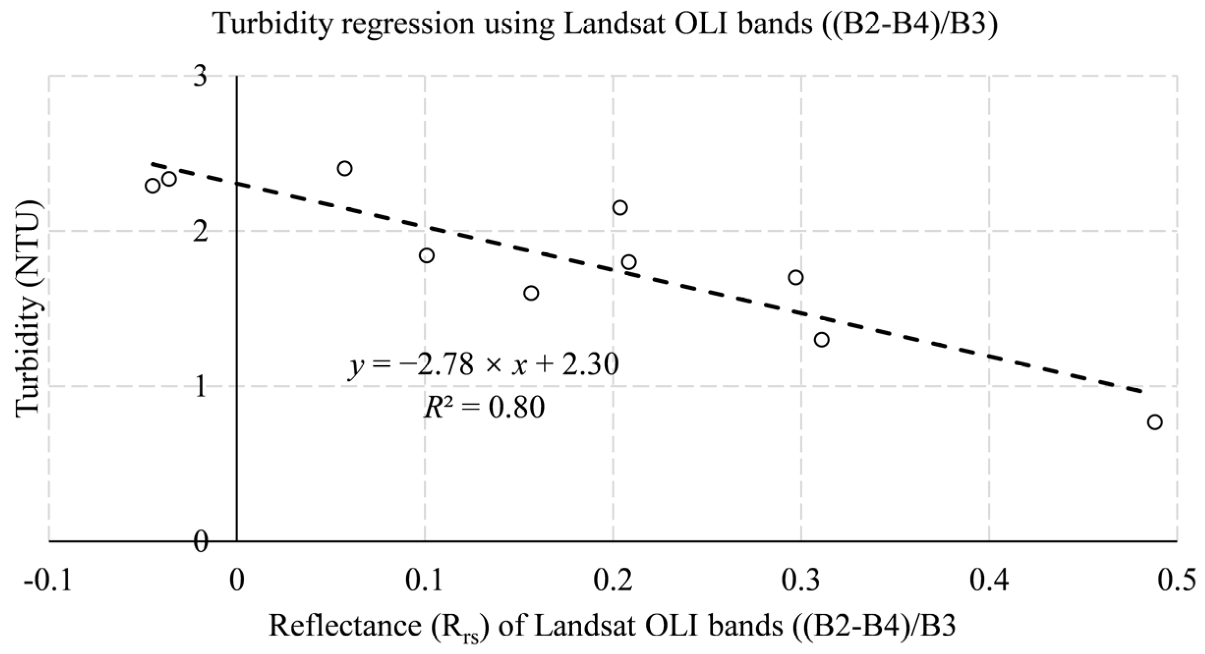
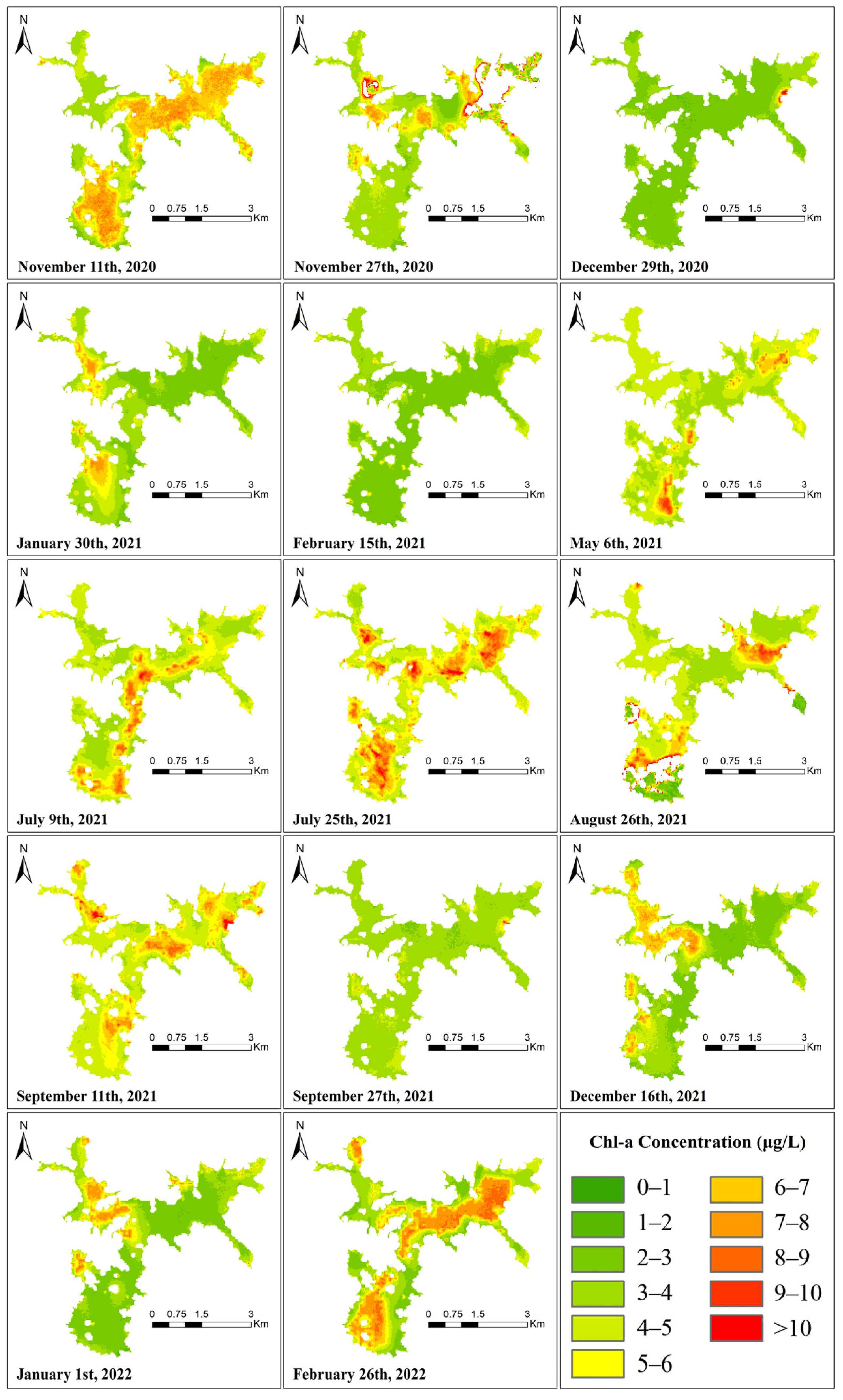
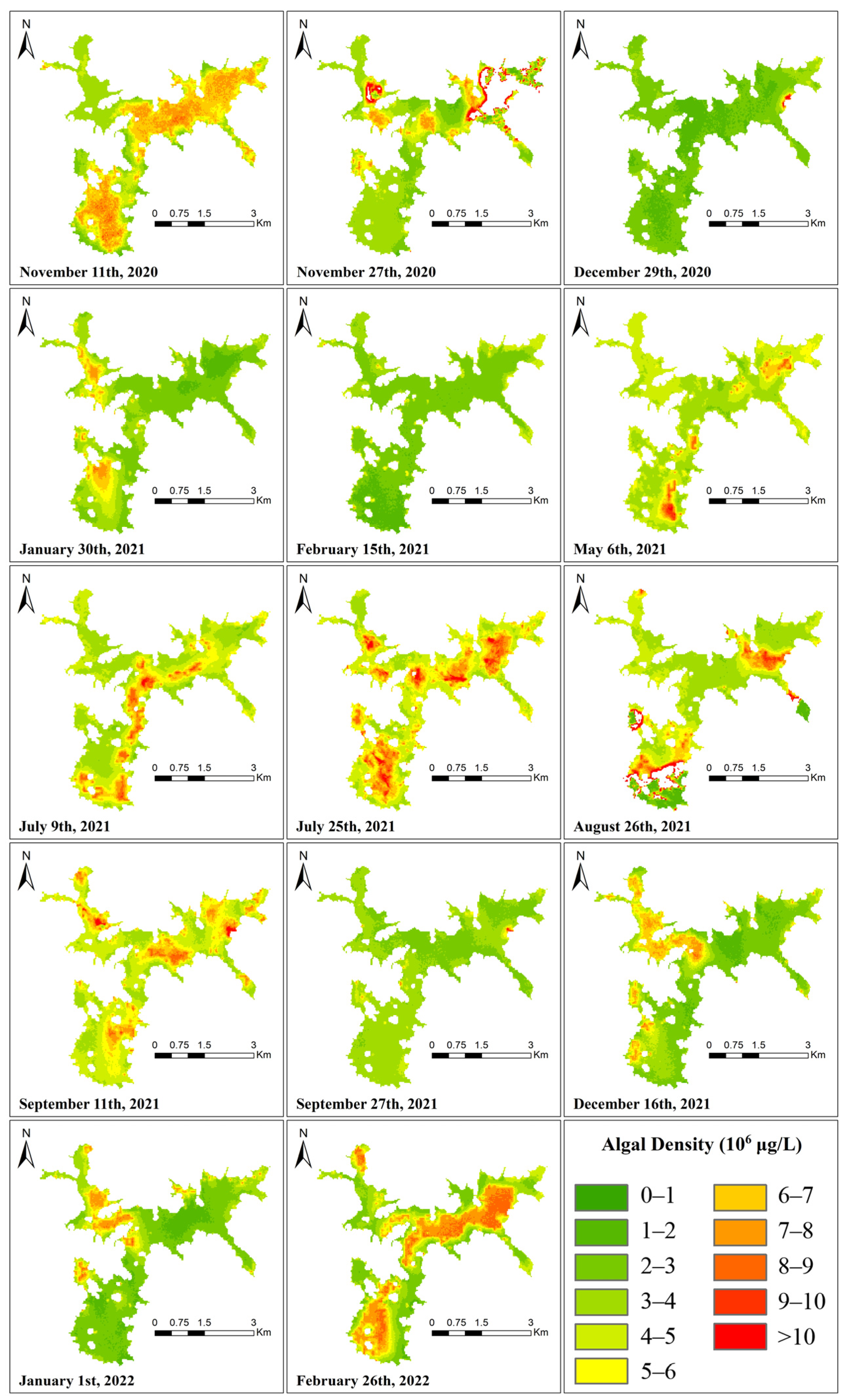
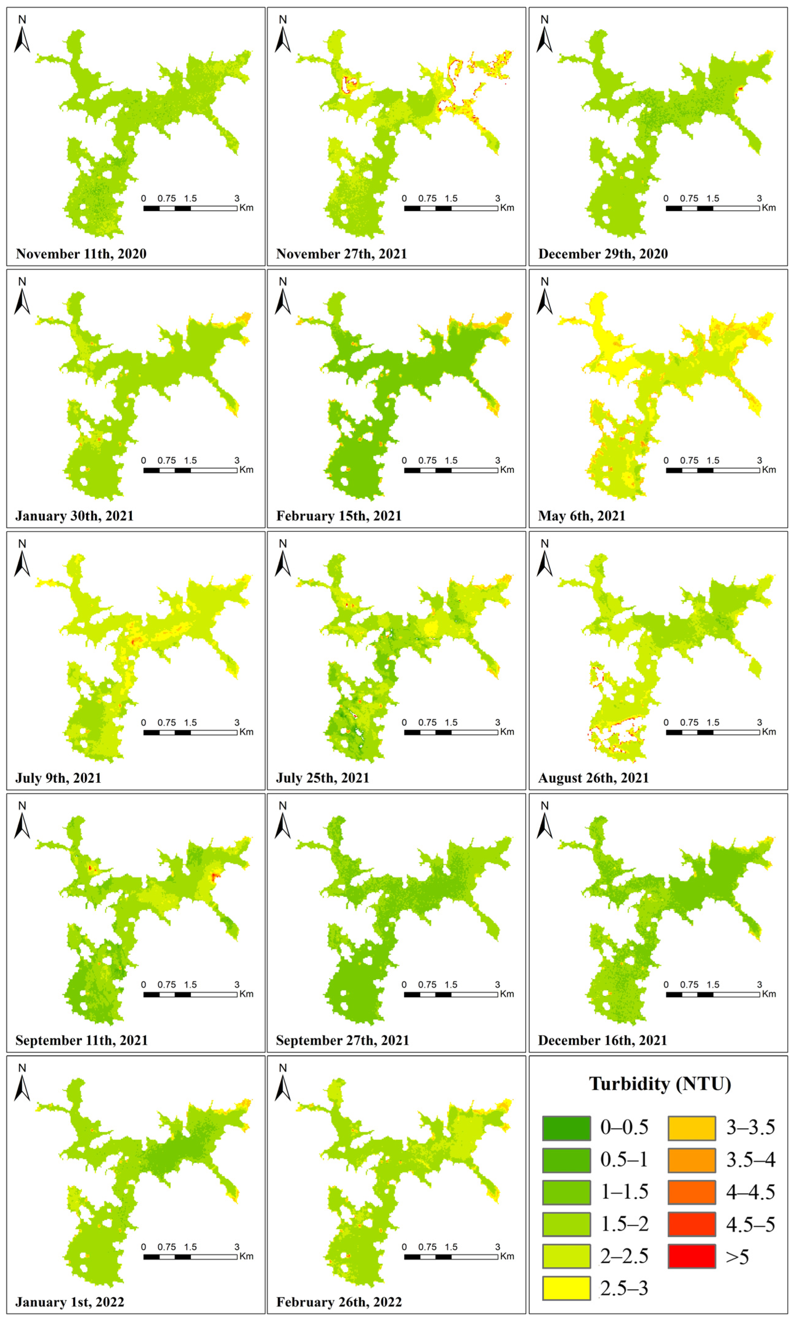
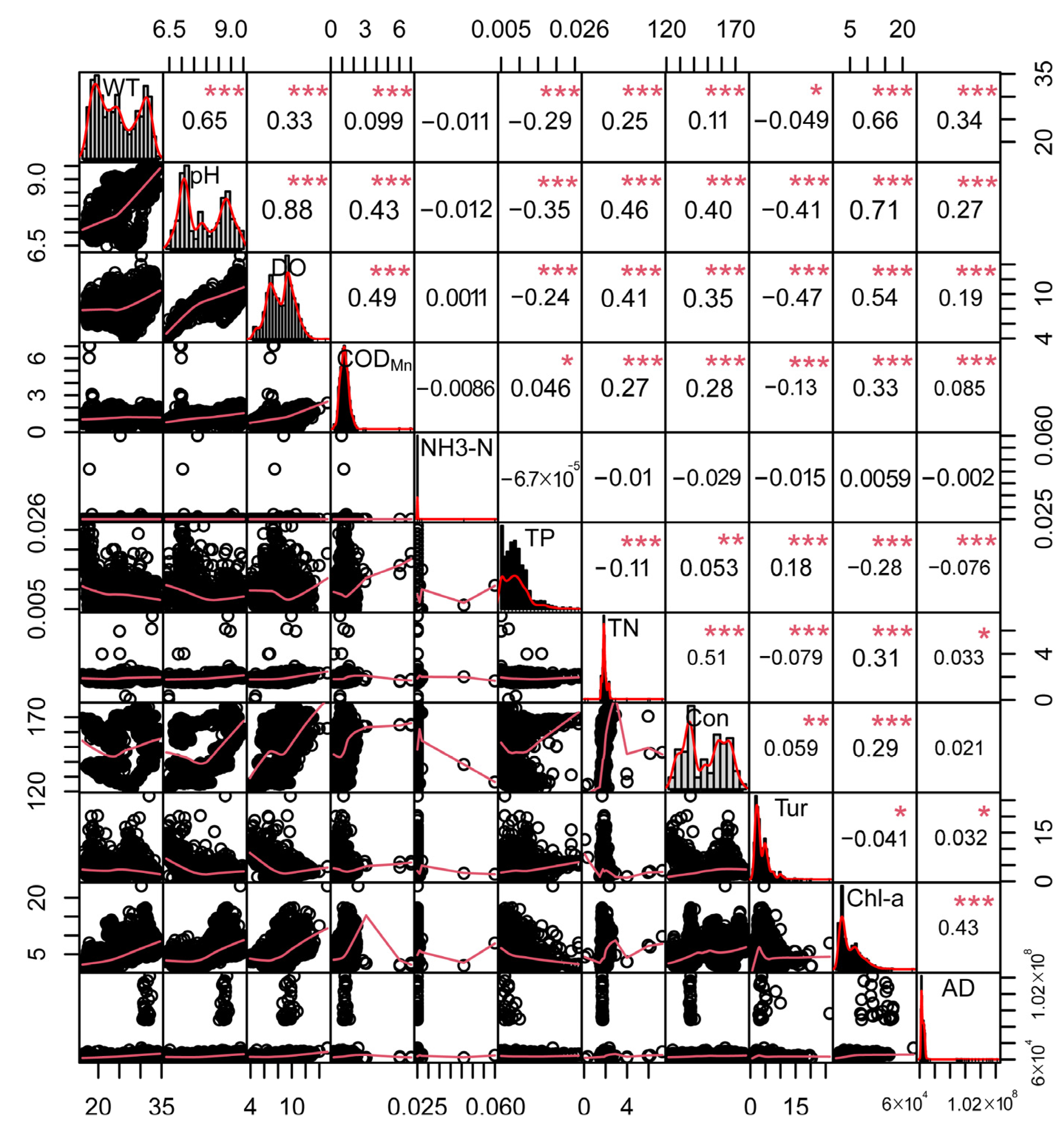
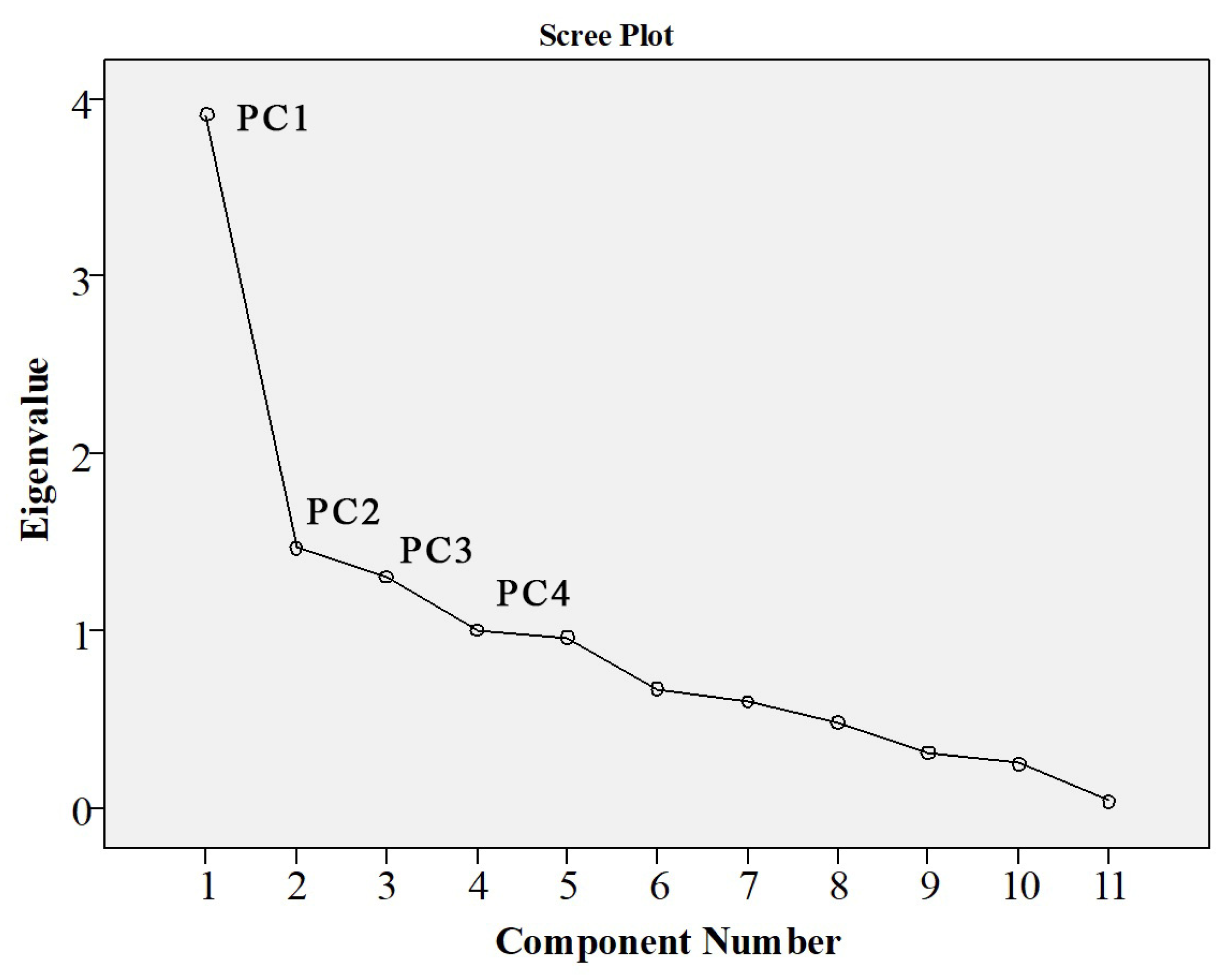
1. Introduction
Inland waters cover approximately 3% of the terrestrial surface of the Earth and have many important functions including providing ecosystem services such as hydroelectric power, flood protection, navigation, water supply, and fisheries [
1,
2]. It is estimated that approximately one in eight global citizens still do not have access to safe drinking water, although access has increased in recent years [
3]. With the water demand in some countries likely to exceed the supply by 50%, nearly half the global population will face water scarcity by 2030 [
4]. Therefore, water resource management is particularly important to ensure that there is a sufficient water quantity of adequate quality for multiple human uses by managing water resources.
Reservoirs are a distinct example of inland water bodies and are transitional systems between rivers and lakes formed by the damming of rivers. Reservoirs are also simple targets for waste disposal [
5]. The biotic and abiotic variables of these functionally complex ecosystems undergo rapid changes owing to natural environmental changes, changes in watershed land cover and land use, and changes in water demand [
6]. The construction and use of reservoirs change the hydrodynamics of rivers, with different impacts on terrestrial and aquatic systems [
7]. With an increase in residence time, the effective utilization time of nutrients is prolonged, and water bodies become increasingly eutrophic [
8]. Therefore, monitoring WQPs is crucial for maintaining the health of these water bodies.
WQPs are usually obtained using in situ sensor probes or by analyzing water samples collected in the field. These traditional methods are laborious, expensive, and have limited spatial coverage [
9]. Remote sensing, with its advantages of broad spatial coverage and repetitive temporal coverage, can complement in situ measurements. Using remote sensing, maps showing the spatial distribution of WQPs can be generated at multiple time intervals for monitoring purposes. Therefore, remote sensing technology, which can simultaneously monitor large areas, has been widely used.
Since the 1960s, remote sensing techniques have been used to monitor aquatic environments by analyzing ocean colors under the assumption that Chl-a (a quantified proxy for phytoplankton biomass) and surface temperature can be estimated remotely [
5,
10]. Based on this, many researchers have used satellite sensors to evaluate WQPs with optically active parameters, such as total suspended matter, Chl-a concentration, turbidity, phytoplankton pigments, and color-dissolved organic matter (CDOM) [
11,
12,
13]. However, estimating TN, TP, and COD concentrations in inland waters presents a great challenge. As the above parameters are not optically active at the sensed wavelengths [
14], it is difficult to directly correlate remote sensing spectral characteristics with TN, TP, and COD concentrations [
15], so most of the current studies using conventional remote sensing monitoring methods focus on WQPs with optical activity. In terms of WQPs retrieval, previous studies were based mainly on different correlation algorithms of empirical, semi-analytical, and matrix retrieval models. Semi-analytical models are based on radiative transfer theory and require bio-optical and empirical data to describe the relationship between the components of a water body and the equivalent surface reflectance that defines the upwelling radiance above and on the surface of the water [
16,
17]. There are three general types of semi-analytical models, one of which is the retrieval and optimization algorithm [
18]. It uses a forward model to simulate spectra from multiple parameters and selects the set of parameters that minimize the chosen cost function as the solution [
19]. If the forward model is linear and the cost function is the sum of the squares of the residuals, this is reduced to the linear matrix retrieval method [
20]. However, owing to the lack of specific parameters, matrix retrieval methods are complicated and difficult to calibrate. Therefore, empirical algorithms are typically employed to retrieve and estimate WQPs [
21,
22].
The continuous development of remote sensing and geographic information science has significantly improved the efficiency of geographical feature analysis [
23,
24,
25]. The increased frequency of image acquisition and advances in data processing capabilities have provided new opportunities for understanding complex inland water systems [
26]. Remote sensing-based assessments and water monitoring may use the same methods for retrieval and prediction, but various sensors can be used for research. For example, the Moderate-Resolution Imaging Spectroradiometer (MODIS), Medium-Resolution Imaging Spectrometer (MERIS), MultiSpectral Instrument (MSI), and Operational Land Imager (OLI) can be used. These sensors are different in spatial, temporal, spectral, and radiometric resolutions, and several studies have been carried out to estimate WQPs using these sensors [
27,
28,
29]. The applicability of WV-2 imagery with existing effective estimation methods from MERIS when estimating the Chl-a concentration in inland turbidity waters was verified for Guanting Reservoir, where the correlation analysis of the measured Chl-a concentration content and WV-2 imagery bands show that the bands of WV-2 sensitive to the Chl-a concentration are red edge, NIR 1, and NIR 2 [
30]. A study on Araucanian lakes developed and validated empirical models to estimate turbidity values from Landsat images and determine the spatial distribution thereof [
31]. Yashon et al. proposed an empirical multivariate regression model (EMRM) algorithmic approach for estimating the Chl-a concentration, total suspended solids (TSS), and turbidity associated with field laboratory measurements; the results showed that the algorithms developed are broadly able to discern the bio-optical quality of water in reservoirs, even if the absolute accuracy of the retrieval of the WQPs still requires improvements [
17]. Using Landsat satellite images, 11 spectral indicators were calculated, and the correlation between the vegetation index and Chl-a concentration in different monitoring areas was established. The indicators with the best correlations were the normalized difference vegetation index (NDVI) and the green normalized difference vegetation index (GNDVI) [
32].
Taking the Shanmei Reservoir in Fujian Province, China, as a case study, the aims of this work were to (1) describe the reflection characteristics of the water body in different bands of the Sentinel MSI and Landsat OLI data combined with the observed water quality data for the reservoir; (2) generate and validate empirical models for WQPs from the two satellite sensors, by comparing the size of validation parameters (MAE, MSE, RMSE), and select the remote sensing inversion model more suitable for the reservoir; (3) retrieve the Chl-a, algal density, and turbidity with optical activity according to the regression formula to understand the current status and changing characteristics of the water quality of the reservoir, and (4) explore the relationship between WQPs, and select the factors that have a greater impact on the water quality, so as to provide a reference for the rapid monitoring of the water quality of the reservoir in the future. Establishing simple models with high accuracy and known errors will facilitate rapid, accurate, and real-time evaluation of water quality using measured data and remote sensing techniques. We hope that this study can provide a reference for the further study of reservoir water quality, which is conducive to the monitoring and early warning of reservoir nutritional status, ensuring the safety of downstream people’s life and farmland water, and creating a better reservoir environment.
4. Discussion
4.1. Analysis of Current Water Quality Status and Relationship between WQPs
It can be seen that there is no obvious seasonal or monthly variation law of the Chl-a concentration, algal density, and turbidity in Shanmei Reservoir. The average annual concentration of Chl-a in the reservoir is 4.25 μg/L. The numerical variation trend of algal density is similar to that of Chl-a concentration, and it is also maintained at a low level. For turbidity, its value and spatial distribution have been kept in a stable state, and the multi-year average is only 1.86 NTU. The retrieval results of the three WQPs also show that the eutrophication level in the study area is low.
On the other hand, as can be seen from the reflectivity of each band in
Figure 3, the reflectivity of the green (B3) band is higher than those of the longer wavelength bands, partly because of atmospheric processes and partly because of the presence of phytoplankton [
35], which explains the peak of the green (B3) band in
Figure 3. In the red-edge (705–782 nm) bands, the lack of phytoplankton makes the peak near the 705 nm wavelength in eutrophic lakes visible, and the peak of reflectance is more obvious. In oligotrophic lakes, the reflectance is close to 0 [
41], which is in line with the characteristics of the oligotrophic state of the Shanmei Reservoir.
However, the spatial distribution of the Chl-a concentration and algal density (
Figure 8 and
Figure 9) showed that there are high local values of Chl-a concentration and algal density at the remaining time points, except 29 December 2020, 15 February 2021, and 27 September 2021. On 11 November 2020, 25 July 2021, 11 September 2021, and 26 February 2022, the values of cha-a and algal density in the whole reservoir are high, indicating that there is still a risk of eutrophication in the reservoir.
It is worth noting that the study area in February is in winter, and the algae density and chlorophyll concentration should normally be at low values, but there are obvious differences between the retrieval images in February 2022 and February 2021. On 15 February 2021, the Chl-a concentration and algae density values were relatively low, and on 26 February 2022, the Chl-a concentration and algae density in the reservoir showed large-area high values. In situ data (
Figure 13) show that the average Chl-a concentration in February 2021 is 2.15, the value in March 2021 is 3.96, and the value in February 2022 is 3.07, but the value in March 2022 increased to 8.11. This shows that starting from the end of February 2022, the eutrophic level of the reservoir begins to increase, and control measures and continuous observation are urgently needed. This also confirms the feasibility and accuracy of remote sensing inversion in reservoir water quality monitoring.
It can also be seen that the Chl-a concentration on 9 July 2021 has only a small number of high values in the middle and south of the reservoir, and the high values have been distributed to the whole region on 25 July, approximately half a month later. The Chl-a concentration and algal density showed the characteristics of a fast diffusion speed and long duration.
Table 14 shows that pH, DO, Chl-a concentration, WT, TN, and COD
Mn dominated PC1, which explained 35.57% of the total variance, and conductivity, algal density, and WT dominated PC2, which accounted for 14.91%, indicating the importance of pH, DO, Chl-a concentration, WT, TN, COD
Mn, and conductivity in estimating water quality in the study area.
At present, the retrieval of the COD
Mn mainly uses conventional satellite remote sensing (such as GF series satellites, Landsat series satellites) [
42,
43], while the retrieval of DO and TN using hyperspectral remote sensing has higher accuracy [
44,
45,
46]. Combined with the results of the above-related studies, it can be considered that the water quality of Shanmei Reservoir can be better evaluated by measuring pH, conductivity, and WT at the monitoring station, or by establishing the regression fitting equations between Chl-a, algae density, and turbidity and DO, COD
Mn, and TN.
4.2. Selection and Applicability Analysis of Retrieval Band and Algorithm
Taimi et al. used the Olushandja dam in Namibia as a case study and developed a retrieval algorithm based on regression analysis using Landsat-8 reflection value and water quality data such as turbidity, TSS, ammonia, TN, TP, and total algae measured on-site. They found that a regression analysis using blue (B2), green (B3), red (B4), and NIR (B5) bands yields good results [
47]. Willibroad et al. compared four established satellite reflectance algorithms to estimate the Chl-a concentration of Lake Chad, and the results showed that the 3BDA algorithm composed of blue (B2), green (B3), and NIR (B4) bands of Landsat-8 has higher accuracy [
48]. Yashon et al. used Sentinel-2 and Landsat-8 data products to evaluate and retrieve Chl-a concentration, suspended particulate matter, and turbidity, and the results showed that Landsat-8 data performed better in retrieving WQPs, and they found that, in blue waters, owing to the high reflectivity of green algae, green and blue bands are suitable for the detection of algal blooms [
17]. In this study, in the regression formula generated using Landsat OLI reflectance and water quality data, the regression formula for Chl-a concentration is associated with blue (B2), green (B3), and red (B4) bands, the algal density regression formula is highly correlated with blue (B2) and green (B3) bands, and the turbidity regression formula is correlated with blue (B2), green (B3), and red (B4) bands, which is consistent with the above conclusion. However,
Figure 4 shows that Landsat OLI data and Sentinel MSI data use the same band combinations, but MAPE values show obvious differences, indicating that the band combinations will show different simulation effects on various remote sensing data, which may also be the reason for the large difference in the accuracy between the two remote sensing data simulation WQPs regression.
The optical properties of inland waters are very different between water bodies, and there are also significant differences within water bodies. These problems hinder the development of inland water algorithms and typically limit their applicability to different water bodies [
5]. Lai et al. retrieved the concentration and distribution of Chl-a in the Guanting Reservoir based on the measured data in different years and Landsat-8 images and 22 algorithm formulas, including SABI, KIVU, Apple, and other vegetation indicators, and found that there was a strong correlation between the pixel values of adjacent reservoirs in the same image, so the Chl-a estimation model can be applied to each other [
49]. Richard et al. evaluated the performance of 29 algorithms that used satellite spectral data to retrieve Chl-a concentration in two temperate inland lakes, to use it as an indicator of the general state of algal density and potential algal density. Although the two lakes differ in background water quality, size, and shape, the results support multiple sensors utilizing a specific set of algorithms to detect potential algal blooms by using Chl-a concentration as a proxy [
50]. Therefore, whether the WQPs regression formula generated in this study can be applied to other reservoirs (near the study area or with some of the same characteristics as the study area) is a future research direction.
4.3. WQPs Regression Formula and Retrieval Error Analysis
The preprocessing process of Landsat OLI data and Sentinel MSI data is very important, and different processing methods will affect the conversion from top of atmosphere (TOA) reflectance to surface reflectance, thus affecting the regression results of WQPs. In this study, the method of downloading and processing data selected the most mainstream method in the current research, so it can ensure the accuracy of the research results to the greatest extent, even if there are still some inevitable errors.
Another instance of error originates from the adjacency effect of the adjacent land pixels, which is known as the border effect. Inland water bodies are surrounded mostly by land, and border effects are especially significant in areas with raised, undulating topography around the water body [
51]. This means that light from objects around the body of the water can change the radiance reaching the sensor, and large parts of the sky may also be blocked by the ground surface (e.g., vegetation) [
5], making it impossible to obtain the true WQPs at the water boundary accurately.
In addition, the date of collection of water quality data can also be a source of error when comparing it with remote sensing data products from different sensors. Because the revisit period of Landsat 8-9 satellite combination is 8 days, and the combination of Sentinel-2A/2B satellites is 5 days, it is difficult to ensure that the data time of the two satellites is completely consistent, which affects the comparative analysis of the WQPs regression equation. Therefore, in addition to achieving good performance in the preprocessing and data regression fitting stages, it is important to ensure that the data collection dates are closer to each other. In this study, WQPs data were obtained daily, but the time difference of remote sensing images caused uncertainty in the fitting of WQPs. Therefore, future research could create a new and more reliable method to quantify changes in WQPs with a higher temporal resolution by combining products from different remote sensing data sources, together with appropriate water quality estimation algorithms. Simultaneously, the different performances of the understanding algorithm and remote sensing image pairs should also be considered. For example, Yashon et al. adjusted the two remote sensing datasets by band adjustment, performed preprocessing such as atmospheric correction and normalized reflectance and then used the standardized data to retrieve reservoir WQPs [
17].
The validity and accuracy of elemental determinations of water quality depend on the satellite sensors used, the methods employed, and the nature of the waters studied. In this study, regression results for Chl-a concentration, algal density, and turbidity demonstrated the potential of optical satellite remote sensing reflectance data for cost-effective, large-scale, and high-frequency use in monitoring optically active water elements. The purpose of remote sensing retrieval of water quality is to provide real-time assessment of current and future water quality monitoring to prevent water quality deterioration. Despite the good water quality of the reservoirs presented in this study, we recommend their continuous monitoring and management through regression simulation and the retrieval of other important WQPs, such as DO, CODMn, and TN, so as to ensure the good water quality of the reservoir.
4.4. Research Limitations and Prospects
Based on the WQPs regression algorithm obtained from a single monitoring point, this study determines the key water quality characteristics of the reservoir and provides a more feasible idea for inland waters with few monitoring points. However, due to the limitation of the number of water quality monitoring stations, the problem of a small amount of matching data is inevitable. The predicted value of water quality obtained by simulation cannot be aptly compared with the actual value of water quality. The actual spatial and numerical changes in water quality are difficult to quantify, and the regression model will also be affected by the amount of data. With the extension of monitoring time, the regression coefficient may change, but when the data reaches a certain amount, a more accurate and stable regression equation can often be obtained. At the same time, the alternation of day and night, temperature, the intensity of human activities, and the action of aquatic organisms will indeed directly or indirectly affect water quality [
52,
53,
54]. However, the transit time of the remote sensing satellites used in this study is in the morning, so the change in water quality at night is not considered. In addition, Sun et al. believe that non-optically active parameters may be highly correlated with optically active substances, such as Chl-a, TSM, and CDOM [
55], so TN, TP, and COD can be estimated remotely [
15]. At present, some scholars have developed several statistical techniques with empirical and machine learning algorithms to determine the relationship between reflectance and non-optically active parameters in inland waters with the help of hyperspectral images [
46,
56]. As mentioned in
Section 4.1, the three WQPs in this study have a certain correlation with some non-optically active water quality parameters (such as DO, COD
Mn, and TN). Therefore, the WQPs of regional non-optically active water quality can be estimated through machine learning algorithms. In the ideal future, the acquisition frequency and accuracy of satellite images will be the same as that of water sample data, so as to reduce the time difference between different satellite images. At the same time, more matching data can be obtained by adding monitoring points or stations at different locations, as was performed by Curtarelli et al. who arranged them in the reservoir near the dam, in the middle of the reservoir, at the tail of the reservoir, and near the tributary [
57]. In addition, the impact on the water quality of inland reservoirs can also be studied in terms of hydrological changes such as water volume and reservoir depth [
58], so as to more comprehensively judge the current status and future trends of reservoir water quality. At the same time, for remote sensing data, preprocessing and adjacency affect the selection or development of corresponding algorithms for correction and the retrieval of more accurate water quality data, which can be used for water resources management and environmental protection planning.
5. Conclusions
This study compared the accuracy of Landsat 8-9 OLI and Sentinel 2 MSI sensors for the retrieval of Chl-a, algal density, and turbidity in the reservoir. Both types of satellite data showed high reflectivity in the green (B3) band. The results of the empirical multiple-regression model show that the R2 and validation parameters (MAE, MSE, and RMSE) of the Landsat OLI fitting equation are better than Sentinel MSI data. Therefore, Landsat OLI data have better application potential in this study area. The 2020–2022 reservoir water quality images retrieved from Landsat OLI data show that the multi-month average values of reservoir WQPs are low. However, from the end of February 2022, the Chl-a concentration and algal density in the reservoir gradually increased, and local high values appeared. Therefore, continuous attention and corresponding water quality management measures are still needed. The results of correlation analysis and principal component analysis show that the water quality of Shanmei Reservoir can be evaluated more accurately and quickly by measuring the pH, conductivity, and WT of the monitoring station, or by establishing the regression fitting equation between Chl-a, algae density, and turbidity and DO, CODMn, and TN. In the future, to improve the accuracy of the estimation of the overall water quality status of the reservoir, new methods can be developed to monitor, fit, and retrieve more factors that can represent the water quality status, or understand the impact of the algorithm on the different performances of remote sensing images to conduct frequent water quality assessments. Simultaneously, we can also apply the regression equation from the study area to verify the accuracy of the regression formula in adjacent waters or similar waters.