
Possibility of Metal Accumulation in Reed Canary Grass (Phalaris arundinacea L.) in the Aquatic Environment of South-Western Polish Rivers

 , and
, and 
Abstract
:1. Introduction
2. Materials and Methods
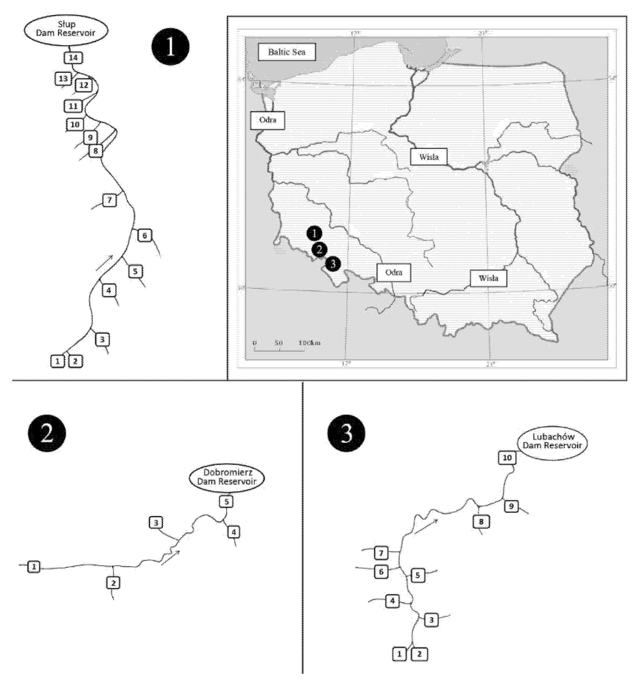
2.1. Study Area
2.2. Material
- Domain: Eucaryota—eukaryotes
- Kingdom: Archaeplastida (Plantae)—plants
- Clade: Spermatophyta—spermatophytes
- Class: Liliopsida (Monocotyledones)—monocotyledons
- Order: Poales (Graminales)—Glumiflorae
- Family: Poeceae (Gramineae)—grasses
- Subfamily: Pooideae
- Tribe: Poeae
- Subtribe: Phalaridinae
- Species: reed canary grass (Phalaris arundinacea L.)
- metals bioaccumulation factor (BCFB) as a ratio of its content in aquatic plant (CP) to its concentration in bottom sediment (CB) [28]
- metals bioaccumulation factor BCFW as a ratio of its content in aquatic plant CP to its concentration in water CW [28]
2.3. Statistical Analysis
3. Results and discussion
3.1. Metals in Reed Canary Grass
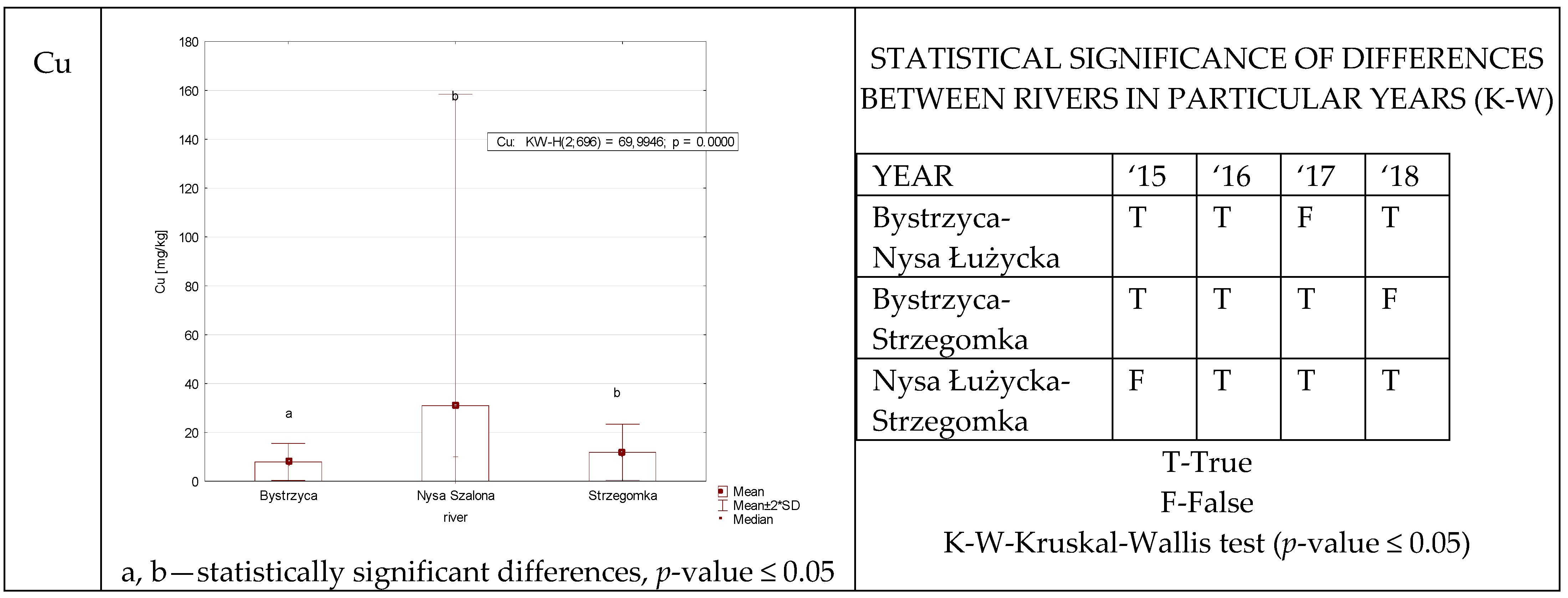
3.1.1. Copper
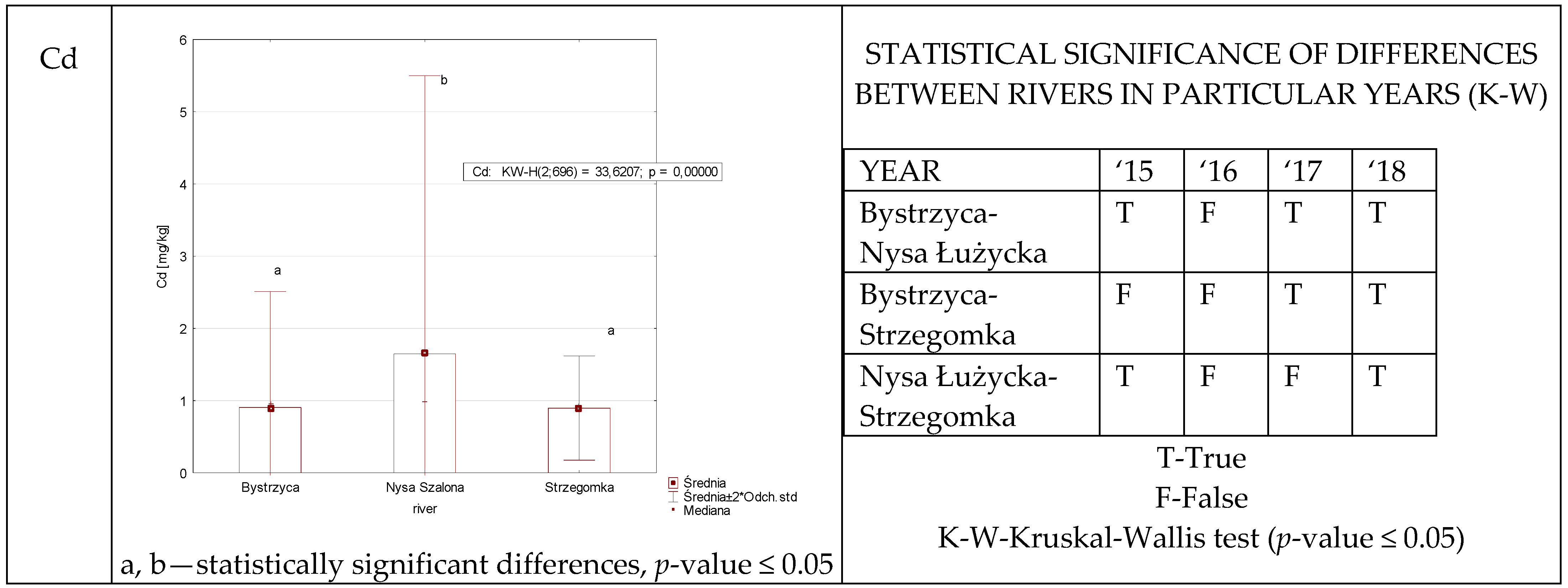
3.1.2. Cadmium
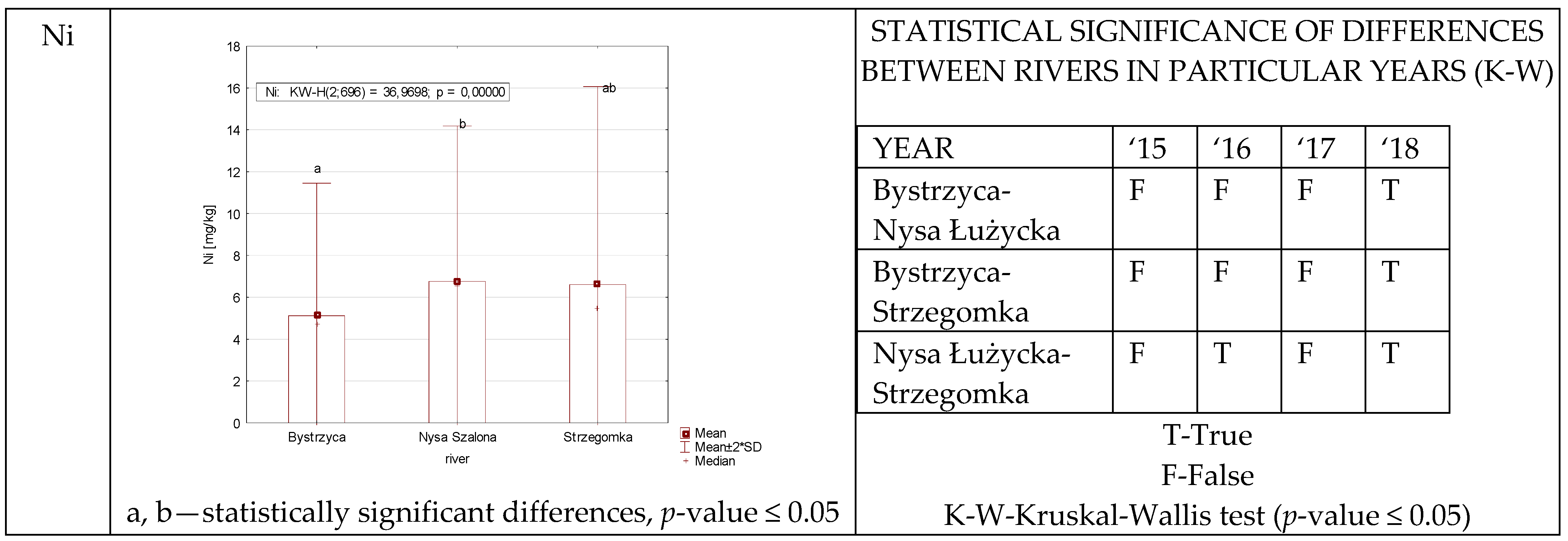
3.1.3. Nickel
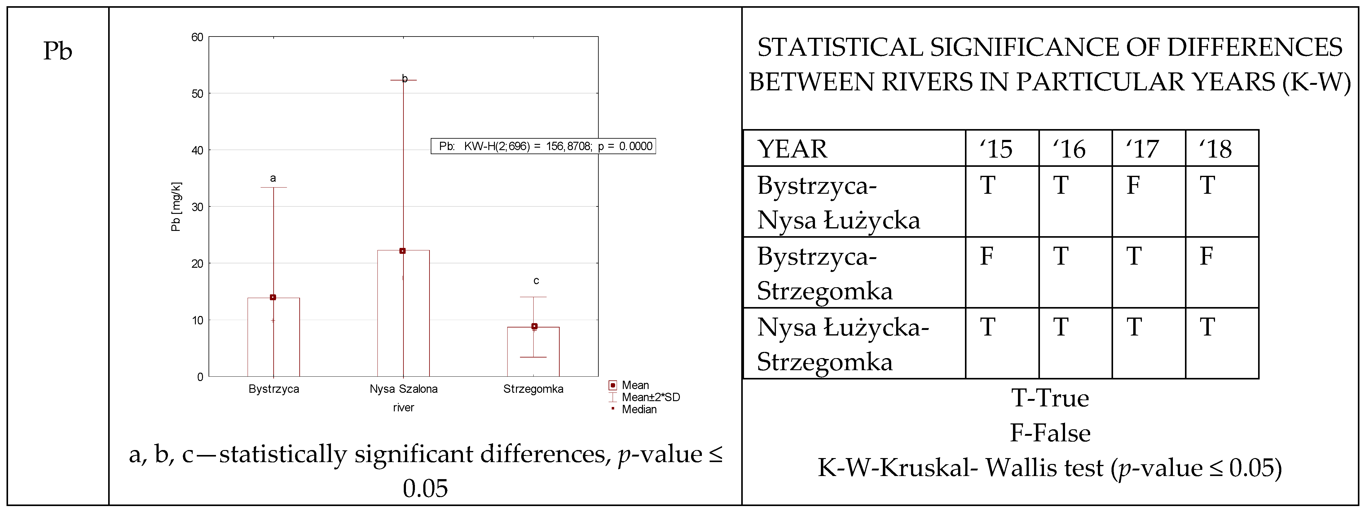
3.1.4. Lead
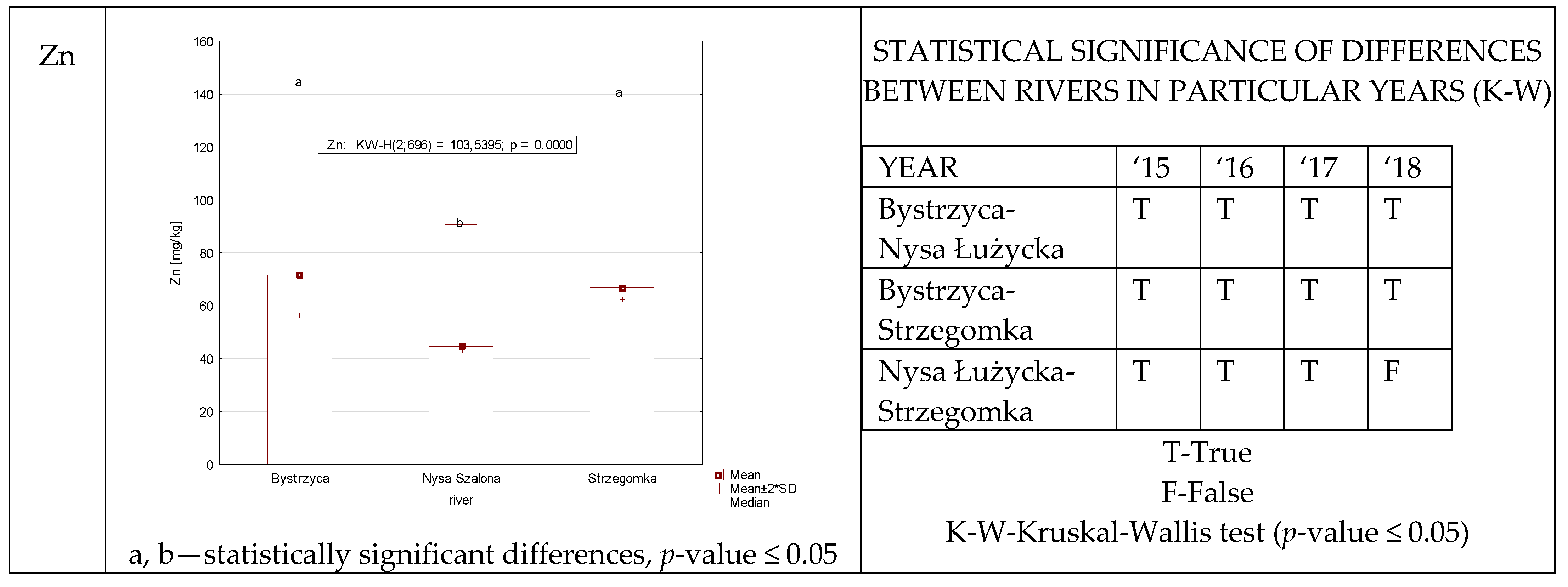
3.1.5. Zinc
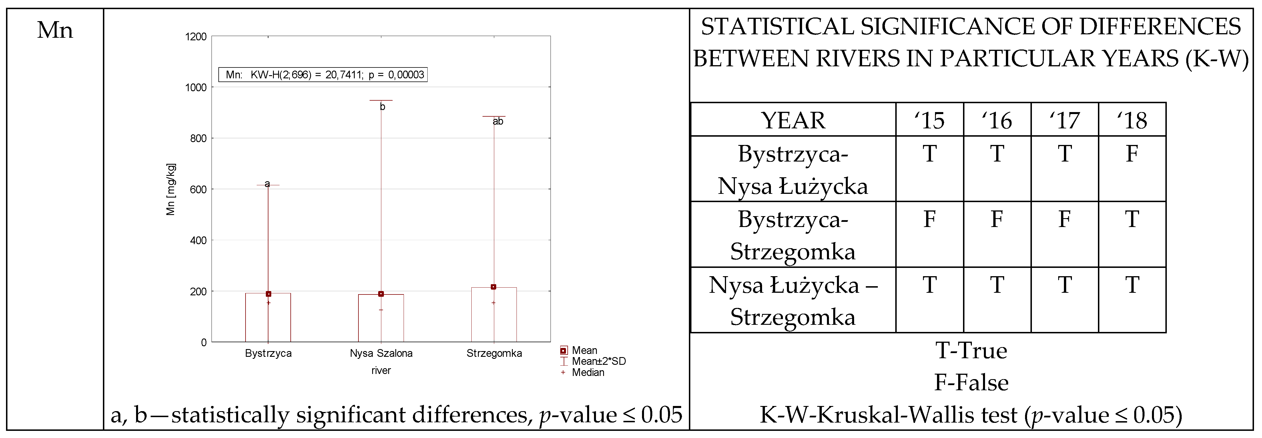
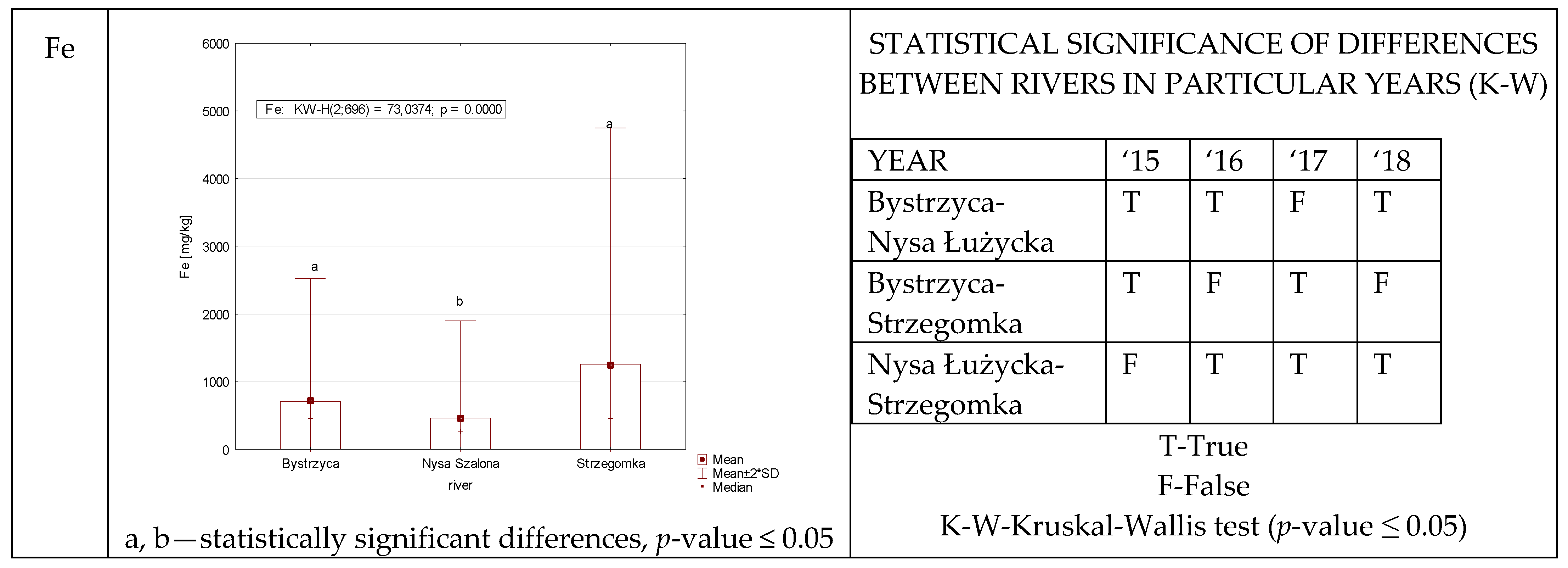
3.1.6. Iron and Manganese
3.2. Comparison of Metals Content—Source and Mouth of the River
3.3. Metals in Tributaries of Major Rivers
3.4. Metal Pollution Index (MPI) and Enrichment Factor (EF)
4. Conclusions
Supplementary Materials
Author Contributions
Funding
Institutional Review Board Statement
Informed Consent Statement
Conflicts of Interest
References
- John, D.A.; Leventhal, J.S. Bioavailability of metals. In Preliminary Compilation of Descriptive Geoenvironmental Mineral Deposit Models; U.S. Department of the Interior, United States Geological Survey: Denver, CO, USA, 1995; pp. 10–18. [Google Scholar]
- Senze, M.; Kowalska-Góralska, M.; Pokorny, P. Metals in chosen aquatic plants in a lowland dam reservoir. J. Elem. 2009, 14, 147–156. [Google Scholar] [CrossRef] [Green Version]
- Gaillardet, J.; Viers, J.; Dupré, B. Trace Elements in River Waters. In Treatise on Geochemistry, 2nd ed.; Springer: Berlin/Heidelberg, Germany, 2014. [Google Scholar] [CrossRef]
- Polechońska, L.; Klink, A. Trace metal bioindication and phytoremediation potentialities of Phalaris arundinacea L. (reed canary grass). J. Geochem. Explor. 2014, 146, 27–33. [Google Scholar] [CrossRef]
- Wojtkowska, M. Heavy metals in water, sediments and plants of the Zegrzyński Lake. Prog. Plant Prot. 2014, 54, 95–101. [Google Scholar] [CrossRef]
- Ciszewski, D.; Malik, I.; Wardas, M. Geomorpfological influences on heavy metal migration in fluvial deposits: The Mała Panew River velley (southern Poland). Przegląd Geol. 2004, 52, 163–174. [Google Scholar]
- Huang, Y.; Zhang, D.; Xu, Z.; Yuan, S.; Li, Y.; Wang, L. Effect of overlying water pH, dissolved oxygen and temperature on heavy metal release from river sediments under laboratory conditions. Arch. Environ. Prot. 2017, 43, 28–36. [Google Scholar] [CrossRef] [Green Version]
- Shi, X.; Zhang, W. Experimental study on release of heavy metals in sediment under hydrodynamic conditions. IOP Conf. Ser. Earth Environ. Sci. 2018, 208, 012040. [Google Scholar] [CrossRef]
- Zhang, Y.; Zhang, H.; Zhang, Z.; Liu, C.; Sun, C.; Zhang, W.; Marhaba, T. pH effect on heavy metal release from a polluted sediment. Hindawi J. Chem. 2018, 2018, 7597640. [Google Scholar] [CrossRef]
- Miranda, L.S.; Wijesiri, B.; Ayoko, G.A.; Egodawatta, P.; Goonetilleke, A. Water-sediment interactions and mobility of heavy metals in aquatic environments. Water Res. 2021, 202, 117386. [Google Scholar] [CrossRef]
- Market, B. Presence and significance of naturally occurring chemical elements of the periodic system in the plant organism and consequences for future investigations on inorganic environmental chemistry in ecosystems. Vegetatio 1992, 103, 1–30. [Google Scholar] [CrossRef]
- Kabata-Pendias, A.; Pendias, H. Biogeochemia Pierwiastków Śladowych, PWN; Scientific Publisher PWN: Warsaw, Poland, 1999. [Google Scholar]
- Kowal, A. Uzdatnianie wody ze zbiornika zaporowego Dobromierz. Ochr. Sr. 1991, 1, 35–38. [Google Scholar]
- Czamara, W.; Krężel, J.; Łomotowski, J. Wpływ retencji zbiornikowej na jakość wody powierzchniowej w zlewni Nysy Szalonej. Zesz. Nauk. Akad. Rol. We Wrocławiu Konf. 1994, 3, 246. [Google Scholar]
- Broś, K. Instrukcja Eksploatacji Zbiornika Słup na Rzece Nysie Szalonej; ODGW: Wrocław, Poland, 1995. [Google Scholar]
- Samecka-Cymerman, A.; Kolon, K.; Kempers, A.J. A comparison of native and transplanted Frontinalis antipyretica Hedw. as biomonitors of water polluted with heavy metals. Sci. Total Environ. 2005, 341, 97–107. [Google Scholar] [CrossRef] [PubMed]
- Senze, M.; Kowalska-Góralska, M.; Czyż, K. Availability of aluminum in river water supplying dam reservoirs in Lower Silesia considering the hydrochemical conditions. Environ. Nanotechnol. Monit. Manag. 2021, 16, 100535. [Google Scholar] [CrossRef]
- Senze, M.; Kowalska-Góralska, M.; Czyż, K.; Wondołowska-Grabowska, A.; Łuczyńska, J. Aluminum in Bottom Sediments of the Lower Silesian Rivers Supplying Dam Reservoirs vs. Selected Chemical Parameters. Int. J. Environ. Res. Public Health. 2021, 18, 13170. [Google Scholar] [CrossRef]
- GIOŚ. Chief Inspectorate of Environmental Protection; Report on the State of the Environment; GIOS: Warsaw, Poland, 2018. [Google Scholar]
- Soil and Agricultural Map; Provincial Centre for Geodetic and Cartographic Documentation: Wrocław, Poland, 2019.
- PN-EN 14184:2014-05; Water Quality-Guidelines for the Study of Hydromacrophytes in Running Waters. Polski Komitet Normalizacyjny: Warsaw, Poland, 2014.
- PN-EN ISO 5667-3:2018-08; Guidelines for the Preservation and Handling of Samples. Polski Komitet Normalizacyjny: Warsaw, Poland, 2018.
- PN-EN ISO 5667-6:2016-12; Water Quality. Sampling. Guidelines for Sampling Rivers and Streams. Polski Komitet Normalizacyjny: Warsaw, Poland, 2016.
- PN-ISO 8288:2002; Water Quality. Determination of Cobalt, Nickel, Copper, Zinc, Cadmium and Lead - Atomic Absorption Spectrometry with Flame Atomization. Polski Komitet Normalizacyjny: Warsaw, Poland, 2002.
- PN-ISO 6332:2001+Ap1:2016-06; Determination of Iron Concentration Spectrophotometric Method. Polski Komitet Normalizacyjny: Warsaw, Poland, 2001.
- PN-92/C-04590/03; Determination of Manganese Concentration Spectrophotometric Method. Polski Komitet Normalizacyjny: Warsaw, Poland, 1992.
- PB-10/I; Test Procedure. VARIAN Analytical Methods.
- Jezierska, B.; Witeska, M. Metal Toxicity to Fish; University of Podlasie: Siedlce, Poland, 2001. [Google Scholar]
- Usero, J.; Gonzales-Regalado, E.; Garcia, I. Trace metals in bivalve molluscs Ruditapes decussatus and Ruditapes philippinarum from the Atlantic Coast of southern Spain. Environ. Int. 1997, 23, 291–298. [Google Scholar] [CrossRef]
- Sutherland, R.A. Bed Sediment-Associated Trace Metals in an Urban Stream, Oahu, Hawaii. Environ. Geol. 2000, 39, 611–627. [Google Scholar] [CrossRef]
- Samecka-Cymerman, A.; Kempers, A.J. Bioindication of heavy metals by Mimulus guttatus from the Czeska Struga Stream in the Karkonosze Mountains, Poland. Bull. Environ. Contam. Toxicol. 1999, 63, 65–72. [Google Scholar] [CrossRef]
- Szymanowska, A.; Samecka-Cymerman, A.; Kempers, A.J. Heavy metals in three lakes in west Poland. Ecotoxycol. Environ. Saf. 1999, 43, 21–29. [Google Scholar] [CrossRef]
- Samecka-Cymerman, A.; Kempers, A.J. Concentrations of heavy metals and plant nutrients in water, sediments and aquatic macrophytes of anthropogenic lakes (former open cut brown coal mines) differing in stage of acidifification. Sci. Total Environ. 2001, 281, 87–98. [Google Scholar] [CrossRef]
- Samecka-Cymerman, A.; Kolon, K.; Kempers, A.J. Heavy metals in aquatic bryophytes from the Ore Mountains (Germany). Ecotoxicol. Environ. Saf. 2002, 52, 203–210. [Google Scholar] [CrossRef]
- Samecka-Cymerman, A.; Kempers, A.J. Biomonitoring of water pollution with Elodea canadensis. A case study of three small Polish rivers with different levels of pollution. Water Air Soil Pollut. 2003, 145, 139–153. [Google Scholar] [CrossRef]
- Rajfur, M.; Kłos, A.; Wacławek, M. Bioaccumulation of heavy metals in aquatic plants the example of Elodea canadensis Michx. Proc. ECOpole 2010, 4, 193–198. [Google Scholar]
- Klink, A.; Macioł, A.; Wisłocka, M.; Krawczyk, J. Metal accumulation and distribution in the organs of Typha latifolia L. (cattail) and their potential use in bioindication. Limnologica 2013, 43, 164–168. [Google Scholar] [CrossRef]
- Pokorny, P.; Pokorny, J.; Dobicki, W.; Senze, M.; Kowalska-Góralska, M. Bioaccumulations of heavy metals in submerged macrophytes in the mountain river Biała Lądecka (Poland, Sudety Mts.). Arch. Env. Prot. 2015, 41, 81–90. [Google Scholar] [CrossRef] [Green Version]
- Klink, A.; Polechońska, L.; Cegłowska, A.; Stankiewicz, A. Typha latifolia (broadleaf cattail) as bioindicator of different types of pollution in aquatic ecosystems—Application of self-organizing feature map (neutral network). Environ. Sci. Pollut. Res. 2016, 23, 14078–14086. [Google Scholar] [CrossRef]
- Samecka-Cymerman, A.; Kempers, A.J. Toxic metals in aquatic plants surviving in surface water polluted by copper mining industry. Ecotoxicol. Environ. Saf. 2004, 59, 64–69. [Google Scholar] [CrossRef]
- Samecka-Cymerman, A.; Kempers, A.J. Bioindications of heavy metals with aquatic macrophytes: The case of a stream polluted with power plant sewages in Poland. J. Toxicol. Environ. Health 2001, 62, 57–67. [Google Scholar] [CrossRef]
- Skorbiłowicz, M.; Wiater, J. Ocena zanieczyszczenia metalami ciężkimi małych cieków wodnych w obszarze Biebrzańskiego Parku Narodowego. Acta Agrophys. 2003, 1, 321–328. [Google Scholar]
- Jastrzębska, M.; Cwynar, P.; Polechoński, R.; Skwara, T. The content of heavy metals (Cu, Ni, Cd, Pb, Zn) in common reed (Phragmites australis) and floating pondweed (Potamogeton natans). Pol. J. Environ. Stud. 2010, 19, 243–246. [Google Scholar]
- Świerk, D.; Szpakowska, B. Occurrence of heavy metals in aquatic macrophytes colonizing small aquatic ecosystem. Ecol. Chem. Eng. S 2011, 18, 369–384. [Google Scholar]
- Bonanno, G. Arundo donax as a potential biomonitor of trace element contamination in water and sediment. Ecotoxicol. Environ. Saf. 2012, 80, 20–27. [Google Scholar] [CrossRef] [PubMed]
- Bonanno, G. Comparative performance of trace element bioaccumulation and biomonitoring in the plant species Typha domingensis, Phragmites australis and Arundo donax. Ecotoxicol. Environ. Saf. 2013, 97, 124–130. [Google Scholar] [CrossRef] [PubMed]
- Matache, M.L.; Marin, C.; Rozylowicz, L.; Tudorache, A. Plants accumulating heavy metals in the Danube river wetlands. J. Environ. Health Sci. Eng. 2013, 11, 1–7. [Google Scholar] [CrossRef] [PubMed] [Green Version]
- Philips, D.P.; Human, L.R.D.; Adams, J.B. Wetland plants as indicators of heavy metal contamination. Mar. Pollut. Bull. 2015, 92, 227–232. [Google Scholar] [CrossRef] [PubMed]
- Gao, J.; Sun, X.; Jiang, W.; Wei, Y.; Guo, J.; Liu, Y.; Zhang, K. Heavy metals in sediments, soils, and aquatic plants from a secondary of the three gorges reservoir region, China. Environ. Sci. Pollut. Res. 2016, 23, 10415–10425. [Google Scholar] [CrossRef] [PubMed]
- Parzych, A.; Sobisz, Z.; Cymer, M. Preliminary research of heavy metals content in aquatic plants from surface water (Northern Poland). Desalination Water Treat. 2016, 57, 1451–1461. [Google Scholar] [CrossRef]
- Senze, M.; Kowalska-Góralska, M.; Czyż, K. Evaluation of the aquatic environment quality of the three rivers of Western Pomerania. Environ. Nanotechnol. Monit. Manag. 2021, 15, 100420. [Google Scholar] [CrossRef]
- Rzymski, P.; Klimaszyk, P.; Niedzielski, P.; Poniedziałek, B. Metal accumulation in sediments and biota in malta Reservoir (Poland). Limnol. Rev. 2013, 13, 163–169. [Google Scholar] [CrossRef] [Green Version]
- Kanclerz, J.; Borowiak, K.; Mleczek, M.; Staniszewski, R.; Lisiak, M.; Janicka, E. Cadmium and lead accumulation in water and macrophytes in an artificial lake. Annu. Set Environ. Prot. 2016, 18, 322–336. [Google Scholar]
- Łojko, R.; Polechońska, L.; Klink, A.; Kosiba, P. Trace metal concentrations and their transfer from sediment to leaves of four common aquatic macrophytes. Environ. Sci. Pollut. Res. 2015, 22, 15123–15131. [Google Scholar] [CrossRef]
- Skorbiłowicz, E. Zinc and lead in bottom sediments and aquatic plants in river Narew. J. Ecol. Eng. 2015, 16, 127–134. [Google Scholar] [CrossRef]
- Bonanno, G. Trace element accumulation and distribution in the organs of Phragmites australis (common reed) and biomonitoring applications. Ecotoxicol. Environ. Saf. 2011, 74, 1057–1064. [Google Scholar] [CrossRef] [PubMed]
- European Commission. Water Law. Act of July 20, 2017. Journal of Laws 2017 Item 1566; European Commission: Brussels, Belgium, 2017. [Google Scholar]
- European Commission. Ordinance of the Minister of Maritime Affairs and Inland Navigation of 29 August 2019 on the Requirements to be Met by Surface Waters Used for Supplying the Population with Water Intended for Human Consumption. Journal of Laws 2019 Item 1747; European Commission: Brussels, Belgium, 2019. [Google Scholar]


| Metal/Unit | Air | Waters | Soils | Plants |
|---|---|---|---|---|
| ng∙m−3 | mg∙dm−3 | mg∙kg−1 | mg∙kg−1 | |
| Cu | 0.03–4900.00 | 0.001–0.020 | 3.00–25.00 | 5.00–30.00 |
| Cd | 0.003–0.60 | 0.00001–0.00002 | 0.0002–0.60 | 0.05–0.20 |
| Ni | 0.10–1.00 | 0.0001–0.0075 | 5.00–22.00 | 0.10–5.00 |
| Pb | 0.50–10.00 | 0.0002–0.0003 | 25.00–40.00 | 0.10–5.00 |
| Zn | 0.002–0.05 | 1.00–110.00 | 10.00–220.00 | 10.00–70.00 |
| Fe | 0.50–6000.00 | 0.01–1.40 | 8000.00–18,000.00 | 50.00–200.00 |
| Mn | 0.02–900.00 | 0.02–0.06 | 100.00–1300.00 | 70.00–500.00 |
| No | Site—Geographical Coordinates | Surface Water Types, Water Categories—Type Code SWB * Status |
|---|---|---|
| 1 | The Nysa Szalona River below the springs in Domanów—N 50°51′38.8261″ E 16°3′54.4715″ | Upland silicate stream with coarse-grained substrate—western 4 natural |
| 2 | Kocik—N 50°52′15.4891″ E 16°4′5.9042″ | |
| 3 | Ochodnik—E 16°5′59.7672″ | |
| 4 | Sadówka—N 50°55′58.609″ E 16°10′11.3627″ | |
| 5 | Czyściel—N 50°57′49.4252″ E 16°13′57.6982″ | |
| 6 | Radynia—N 50°58′56.648″ E 16°14′13.9202″ | |
| 7 | Nysa Mała—N 51°0′10.455″ E 16°12′26.0825″ | Upland carbonate stream with coarse-grained substrate 7 natural |
| 8 | Puszówka—N 51°2′30.3945″ E 16°11′39.425″ | |
| 9 | Jawornik—N 51°2′57.6884″ E 16°10′52.4584″ | |
| 10 | Księginka—N 51°3′17.4033″ E 16°10′11.2082″ | |
| 11 | Starucha—N 51°4′31.7745″ E 16°9′17.7528″ | Upland silicate stream with fine-grained substrate—western 5 natural |
| 12 | Rowiec—N 51°4′22.844″ E 16°8′27.5419″ | |
| 13 | Męcinka—N 51°4′29.2507″ E 16°7′28.5247″ | |
| 14 | Nysa Szalona mouth to the Słup reservoir— N 51°4′29.2507″ E 16°7′28.5247″ | Small upland silicate river—western 8 artificial watercourse |
| No | Site—Geographical Coordinates | Surface Water Types, Water Categories—Type Code SWB * Status |
|---|---|---|
| 1 | The Strzegomka River below the springs in Nowe Bogaczowice—N 50°50′14.5978″ E 16°7′49.845″ | Upland silicate stream with coarse-grained substrate—western 4 artificial |
| 2 | Polska Woda—N 50°52′48.0601″ E 16°11′56.4194″ | |
| 3 | Sikorka—N 50°51′47.2613″ E 16°13′21.3918″ | |
| 4 | Czyżynka—N 50°52′15.8303″ E 16°14′29.8332″ | |
| 5 | Strzegomka mouth to the Dobromierz reservoir—N 50°53′11.1994″ E 16°13′58.4707″ | Upland silicate stream with coarse-grained substrate—western 4 artificial |
| No | Site—Geographical Coordinates | Surface Water Types, Water Categories—Type Code SWB * Status |
|---|---|---|
| 1 | The Bystrzyca River below the springs in Wrześnik— N 50°38′10.1652″ E 16°24′5.7915″ | Upland silicate stream with coarse-grained substrate—western 4 artificial |
| 2 | Złoty Potok—N 50°38′29.3697″ E 16°24′41.0163″ | |
| 3 | Kłobia—N 50°40′9.374″ E 16°23′27.0131″ | |
| 4 | Otłuczyna—N 50°40′36.2015″ E 16°22′46.8444″ | |
| 5 | Potok Marcowy Duży—N 50°41′5.2762″ E 16°22′32.3218″ | |
| 6 | Złota Woda—N 50°41′4.2973″ E 16°22′11.0015″ | |
| 7 | Rybna—N 50°41′49.8085″ E 16°21′58.1784″ | |
| 8 | Jaworzynik—N 50°43′25.8799″ E 16°23′56.5218″ | |
| 9 | Walimianka—N 50°43′49.9381″ E 16°24′15.0612″ | |
| 10 | Bystrzyca mouth to the Lubachów reservoir— N 50°45′5.8065″ E 16°25′1.4097″ | Upland silicate stream with coarse-grained substrate—western 4 artificial |
| Metal | River | Index | 2015 | 2016 | 2017 | 2018 |
|---|---|---|---|---|---|---|
| Min–Max ± SD | ||||||
| Cu | NS | P | 3.69–396.55 92.79 ± 105.07 | 4.96–19.74 9.40 ± 2.99 | 2.33–20.98 10.85 ± 4.90 | 3.44–27.89 11.04 ± 5.80 |
| 31.02 ± 63.63 | ||||||
| BCFB | 0.0090–13.13 2.92 ± 3.63 | 0.0190–0.5860 0.1550 ± 0.15 | 0.0596–2.12 0.8538 ± 0.58 | 0.1037–1.58 0.5280 ± 0.34 | ||
| 1.11 ± 2.14 | ||||||
| BCFW | 923.00–82,142.29 19,842.46 ± 23,950.61 | 56.26–232.98 134.06 ± 46.13 | 664.66–5878.06 2637.96 ± 1622.71 | 40.60–2045.71 319.32 ± 373.18 | ||
| 5733.45 ± 14,540.62 | ||||||
| B | P | 3.36–15.89 8.15 ± 2.95 | 3.96–9.00 6.66 ± 1.30 | 2.89–23.78 10.09 ± 5.83 | 3.45–13.47 6.76 ± 2.26 | |
| 7.92 ± 3.78 | ||||||
| BCFB | 0.0154–2.77 0.4269 ± 0.59 | 0.0107–1.14 0.3214 ± 0.29 | 0.2479–2.97 0.8282 ± 0.66 | 0.0982–1.63 0.6413 ± 0.42 | ||
| 0.5545 ± 0.55 | ||||||
| BCFW | 437.38–15,894.30 3916.17 ± 2871.31 | 919.94–5736.77 1896.46 ± 1042.13 | 484.54–4634.65 2360.48 ± 1148.15 | 32.31–247.52 92.79 ± 47.97 | ||
| 2066.48 ± 2126.21 | ||||||
| S | P | 9.41–13.98 11.74 ± 1.31 | 8.07–29.89 16.47 ± 7.26 | 9.34–22.68 13.59 ± 3.55 | 3.02–7.93 5.75 ± 1.58 | |
| 11.89 ± 5.72 | ||||||
| BCFB | 0.6326–1.99 1.24 ± 0.38 | 0.6109–4.25 1.57 ± 1.00 | 0.9014–2.24 1.32 ± 0.37 | 0.2281–1.11 0.5561 ± 0.26 | ||
| 1.17 ± 0.69 | ||||||
| BCFW | 1300.77–5589.87 2385.15 ± 1255.77 | 1832.68–4519.43 3133.91 ± 904.62 | 1355.33–9448.13 3102.78 ± 2409.48 | 30.47–157.37 86.93 ± 44.08 | ||
| 2177.04 ± 1896.46 | ||||||
| Cd | NS | P | 0.5964–9.87 3.64 ± 3.05 | 0.5632–1.96 0.99 ± 0.26 | 0.4512–1.83 1.07 ± 0.29 | 0.5612–1.13 0.8932 ± 0.16 |
| 1.65 ± 1.92 | ||||||
| BCFB | 0.1021–21.78 4.95 ± 5.92 | 0.1091–7.85 1.02 ± 1.45 | 0.4114–2.4820 1.11 ± 0.44 | 0.4733–41.07 1.21 ± 4.37 | ||
| 2.09 ± 4.10 | ||||||
| BCFW | 504.68–10,256.00 3665.21 ± 2645.85 | 265.50–9652.00 1602.14 ± 1800.53 | 760.50–15,345.00 3877.44 ± 3409.34 | 13.96–1447.43 70.79 ± 242.36 | ||
| 2303.89 ± 2816.61 | ||||||
| B | P | 0.22–1.24 0.76 ± 0.30 | 0.6312–10.89 1.09 ± 1.28 | 0.8712–2.09 1.31 ± 0.31 | 0.04–2.34 0.45 ± 0.57 | |
| 0.9046 ± 0.80 | ||||||
| BCFB | 0.2575–4.09 0.9804 ± 0.86 | 0.2020–10.86 1.60 ± 1.70 | 0.6409–3.24 1.67 ± 0.74 | 0.0209–2.20 0.50 ± 0.57 | ||
| 1.1860 ± 1.17 | ||||||
| BCFW | 35.85–12,389.00 2785.70 ± 2956.48 | 1308.33–18,155.50 4291.59 ± 3190.04 | 1244.57–16,091.00 6401.30 ± 5395.53 | 71.40–12,385.00 1626.52 ± 2633.81 | ||
| 3776.28 ± 4114.76 | ||||||
| S | P | 0.74–1.16 0.92 ± 0.12 | 0.7412–1.25 0.93 ± 0.13 | 0.1111–2.08 1.05 ± 0.52 | 0.1111–1.45 0.69 ± 0.39 | |
| 0.8969 ± 0.36 | ||||||
| BCFB | 0.8831–1.71 1.25 ± 0.25 | 0.8567–2.21 1.44 ± 0.37 | 0.1297–2.99 1.59 ± 0.92 | 0.1297–1.68 0.7913 ± 0.45 | ||
| 1.27 ± 0.63 | ||||||
| BCFW | 534.06–8644.00 1909.34 ± 2268.10 | 828.58–7532.00 2320.29 ± 1560.09 | 185.17–17,076.00 2870.36 ± 4765.91 | 5.35–44.55 18.16 ± 9.89 | ||
| 1779.54 ± 2953.55 | ||||||
| Ni | NS | P | 0.2654–15.66 5.46 ± 5.33 | 3.25–9.35 6.46 ± 1.62 | 3.34–18.44 7.98 ± 3.22 | 1.72–14.84 7.15 ± 3.18 |
| 6.76 ± 3.71 | ||||||
| BCFB | 0.0061–0.0787 0.0233 ± 0.01 | 0.0059–0.3128 0.1006 ± 0.10 | 0.0663–0.8549 0.2922 ± 0.17 | 0.0212–0.5079 0.1891 ± 0.11 | ||
| 0.1513 ± 0.15 | ||||||
| BCFW | 63.16–13,014.50 4904.16 ± 4274.31 | 21.91–200.52 86.29 ± 45.55 | 146.06–5273.90 1740.10 ± 868.51 | 12.74–943.87 100.54 ± 185.67 | ||
| 1707.77 ± 2936.45 | ||||||
| B | P | 1.63–8.27 4.38 ± 1.95 | 3.34–9.46 6.22 ± 1.60 | 3.73–13.98 8.09 ± 3.11 | 0.1625–4.35 1.81 ± 1.54 | |
| 5.12 ± 3.16 | ||||||
| BCFB | 0.0061–1.12 0.2746 ± 0.31 | 0.0187–0.9039 0.3287 ± 0.27 | 0.1189–1.03 0.4492 ± 0.23 | 0.0041–0.3889 0.1081 ± 0.10 | ||
| 0.2900 ± 0.27 | ||||||
| BCFW | 1088.07–8872.25 4070.95 ± 2000.95 | 2224.60–7880.50 3777.76 ± 1349.49 | 199.35–3233.07 1870.45 ± 765.77 | 0.7329–42.14 16.66 ± 14.51 | ||
| 2408.95 ± 2049.19 | ||||||
| S | P | 4.42–9.07 6.11 ± 1.26 | 2.95–8.49 5.29 ± 1.63 | 4.37–31.67 10.85 ± 7.58 | 2.88–6.91 4.16 ± 1.06 | |
| 6.60 ± 4.71 | ||||||
| BCFB | 0.2072–0.3550 0.2884 ± 0.05 | 0.1305–0.3908 0.2518 ± 0.08 | 0.2241–1.57 0.5080 ± 0.37 | 0.1356–0.3515 0.1990 ± 0.06 | ||
| 0.3111 ± 0.23 | ||||||
| BCFW | 28.32–2108.77 700.64 ± 709.76 | 717.68–2178.60 1311.65 ± 364.22 | 30.77–7256.98 1648.45 ± 2182.31 | 15.35–51.48 29.99 ± 8.54 | ||
| 922.69 ± 1315.60 | ||||||
| Pb | NS | P | 13.00–87.36 36.82 ± 18.85 | 10.43–29.88 16.65 ± 4.04 | 6.02–38.65 16.82 ± 7.75 | 1.73–47.55 18.74 ± 13.53 |
| 22.26 ± 15.00 | ||||||
| BCFB | 0.0513–2.76 0.6813 ± 0.75 | 0.0185–0.8832 0.3040 ± 0.26 | 0.1039–3.79 0.9058 ± 0.89 | 0.1027–1.86 0.7196 ± 0.45 | ||
| 0.6527 ± 0.6734 | ||||||
| BCFW | 245.43–56,963.20 15,757.36 ± 15,294.00 | 3257.25–8316.06 5692.71 ± 1346.02 | 2153.48–48,141.50 14,263.33 ± 9914.17 | 6.03–8807.83 362.88 ± 1528.85 | ||
| 9019.07 ± 11,127.08 | ||||||
| B | P | 2.41–16.07 5.91 ± 3.24 | 17.43–42.85 25.71 ± 6.98 | 8.45–28.95 17.57 ± 5.60 | 1.63–11.51 6.29 ± 2.84 | |
| 13.87 ± 9.72 | ||||||
| BCFB | 0.0013–0.2969 0.0645 ± 0.07 | 0.0099–0.8208 0.2841 ± 0.24 | 0.0736–0.5899 0.3056 ± 0.14 | 0.0102–0.1984 0.0988 ± 0.05 | ||
| 0.1880 ± 0.18 | ||||||
| BCFW | 471.17–38,613.00 5355.71 ± 7137.87 | 7812.33–24,963.20 18,932.01 ± 3872.30 | 2224.36–219,934.00 21,749.61 ± 39,393.70 | 549.78–7290.42 2811.04 ± 1588.59 | ||
| 12,212.09 ± 21,747.66 | ||||||
| S | P | 4.37–12.05 7.64 ± 2.08 | 5.13–14.65 9.02 ± 2.66 | 5.63–15.98 10.26 ± 3.03 | 3.91–10.94 8.02 ± 1.81 | |
| 8.74 ± 2.64 | ||||||
| BCFB | 0.0457–0.3607 0.1495 ± 0.08 | 0.0515–0.2591 0.1313 ± 0.06 | 0.0843–0.4159 0.1948 ± 0.1056 | 0.0618–0.2174 0.1121 ± 0.04 | ||
| 0.1512 ± 0.08 | ||||||
| BCFW | 1213.83–11,348.50 3983.48 ± 2733.79 | 2052.88–12,733.14 5682.49 ± 3019.55 | 2157.64–25,128.60 6934.89 ± 6275.36 | 11.34–78.23 34.89 ± 14.68 | ||
| 4158.93 ± 4556.24 | ||||||
| Zn | NS | P | 5.96–66.87 33.04 ± 18.70 | 22.03–70.01 44.32 ± 13.06 | 25.68–128.72 64.89 ± 28.20 | 15.09–69.74 35.91 ± 13.79 |
| 44.54 ± 23.06 | ||||||
| BCFB | 0.0099–0.9874 0.1400 ± 0.18 | 0.0142–0.9100 0.2511 ± 0.25 | 0.2652–3.1315 1.2300 ± 0.75 | 0.0632–0.9774 0.4465 ± 0.23 | ||
| 0.5212 ± 0.60 | ||||||
| BCFW | 207.77–4399.61 1792.75 ± 1358.27 | 102.25–5303.62 1814.21 ± 1748.98 | 420.79–14,967.59 4391.97 ± 2962.07 | 13.84–2398.60 246.62 ± 424.87 | ||
| 2061.39 ± 2383.09 | ||||||
| B | P | 16.89–120.04 49.67 ± 23.52 | 46.43–169.49 110.38 ± 34.88 | 27.22–134.79 79.20 ± 32.27 | 25.63–80.08 47.46 ± 15.14 | |
| 714.68 ± 37.63 | ||||||
| BCFB | 0.0175–2.22 0.5072 ± 0.55 | 0.0287–3.46 1.42 ± 1.16 | 0.3857–2.77 1.37 ± 0.71 | 0.1492–1.99 0.83 ± 0.47 | ||
| 1.03 ± 0.86 | ||||||
| BCFW | 469.27–29,163.40 3626.89 ± 5641.92 | 2159.59–12,726.10 6461.84 ± 3094.85 | 1645.91–6989.95 3981.76 ± 1648.14 | 42.28–1513.40 375.09 ± 305.49 | ||
| 3611.39 ± 3967.21 | ||||||
| S | P | 43.01–85.70 62.17 ± 14.23 | 39.01–102.68 66.82 ± 20.11 | 57.01–206.54 104.34 ± 44.68 | 10.00–70.27 34.06 ± 20.99 | |
| 66.85 ± 37.24 | ||||||
| BCFB | 0.6694–1.78 1.12 ± 0.36 | 0.4520–2.01 0.9852 ± 0.46 | 0.8359–3.26 1.79 ± 0.65 | 0.1318–1.05 0.4766 ± 0.30 | ||
| 1.09 ± 0.66 | ||||||
| BCFW | 627.36–5909.00 2432.90 ± 1845.40 | 2933.10–70,158.80 10,306.37 ± 1815.65 | 3369.96–12,008.30 6014.73 ± 2400.19 | 21.00–630.48 215.14 ± 203.81 | ||
| 4742.30 ± 9901.70 | ||||||
| Fe | NS | P | 2.96–541.53 199.89 ± 204.39 | 65.01–616.59 208.14 ± 123.18 | 16.32–2946.99 1056.19 ± 850.94 | 46.44–4985.87 381.03 ± 889.57 |
| 461.31 ± 718.53 | ||||||
| BCFB | 0.0001–0.1691 0.0168 ± 0.02 | 0.0031–0.0529 0.0152 ± 0.0125 | 0.0010–0.2993 0.0731 ± 0.0767 | 0.0030–0.2074 0.0217 ± 0.04 | ||
| 0.0320 ± 0.05 | ||||||
| BCFW | 1.23–1694.00 370.14 ± 443.67 | 49.48–4101.20 524.91 ± 791.51 | 24.94–10,035.41 1754.27 ± 1980.97 | 29.51–2413.32 484.94 ± 529.89 | ||
| 783.57 ± 1254.75 | ||||||
| B | P | 156.34–632.98 355.48 ± 112.80 | 198.01–1002.88 487.69 ± 207.04 | 72.08–5081.90 1658.29 ± 1405.45 | 87.11–695.86 331.00 ± 189.35 | |
| 708.12 ± 906.19 | ||||||
| BCFB | 0.0185–0.1030 0.0385 ± 0.02 | 0.0158–3.53 0.1568 ± 0.63 | 0.0073–0.5283 0.1763 ± 0.16 | 0.0049–2.99 0.9449 ± 1.02 | ||
| 0.3291 ± 0.70 | ||||||
| BCFW | 162.09–2758.79 360.43 ± 326.26 | 227.70–3209.08 564.85 ± 627.11 | 157.37–4535.96 1813.98 ± 1480.39 | 32.82–3261.00 719.64 ± 792.59 | ||
| 864.72 ± 1070.73 | ||||||
| S | P | 125.32–252.99 176.01 ± 39.04 | 256.00–1654.80 654.29 ± 409.43 | 393.01–6597.40 3742.4 ± 1860.3 | 108.81–1163.50 457.15 ± 345.08 | |
| 1257.50 ± 1739.10 | ||||||
| BCFB | 0.0088–0.0255 0.0137 ± 0.01 | 0.0131–6.92 1.44 ± 2.09 | 0.0338–0.4875 0.2921 ± 0.15 | 0.0067–1.51 0.4918 ± 0.55 | ||
| 0.5611 ± 1.21 | ||||||
| BCFW | 153.41–609.57 364.94 ± 170.57 | 376.31–4001.80 1227.60 ± 987.62 | 1318.67–16,874.94 7230.87 ± 4190.34 | 99.17–2943.52 841.75 ± 832.42 | ||
| 2416.30 ± 3554.50 | ||||||
| Mn | NS | P | 95.63–637.51 245.13 ± 126.18 | 16.49–369.65 81.24 ± 69.17 | 31.43–883.94 148.99 ± 168.06 | 13.06–3955.12 270.44 ± 711.32 |
| 186.45 ± 380.10 | ||||||
| BCFB | 0.5156–2.76 1.52 ± 0.66 | 0.0968–1.30 0.4800 ± 0.31 | 0.0901–4.96 1.03 ± 0.96 | 0.0681–14.00 1.38 ± 2.50 | ||
| 1.08 ± 1.46 | ||||||
| BCFW | 177.98–20,701.61 2870.61 ± 4592.15 | 61.28–3252.45 608.91 ± 635.14 | 59.91–7864.23 998.85 ± 1398.14 | 90.51–21,392.88 1853.58 ± 3840.08 | ||
| 1582.98 ± 3209.89 | ||||||
| B | P | 110.03–189.34 114.61 ± 20.37 | 128.09–196.99 166.63 ± 16.63 | 35.44–1731.87 339.43 ± 380.89 | 32.58–198.63 114.55 ± 51.16 | |
| 191.30 ± 211.55 | ||||||
| BCFB | 0.6932–7.32 2.84 ± 1.97 | 0.9175–4.30 2.26 ± 1.03 | 0.1126–20.84 2.82 ± 4.35 | 0.2788–35.58 11.25 ± 11.54 | ||
| 4.79 ± 7.29 | ||||||
| BCFW | 389.10–1623.80 913.29 ± 352.49 | 233.95–1419.03 687.73 ± 342.06 | 43.64–6050.89 937.72 ± 1170.59 | 129.17–2254.06 867.17 ± 540.35 | ||
| 851.48 ± 696.75 | ||||||
| S | P | 102.11–156.66 134.22 ± 18.73 | 132.66–175.41 156.74 ± 14.17 | 95.05–2155.80 505.61 ± 569.06 | 12.03–195.91 57.73 ± 60.57 | |
| 213.58 ± 334.35 | ||||||
| BCFB | 0.6215–1.28 0.9692 ± 0.23 | 0.6333–10.67 5.01 ± 4.09 | 0.5574–13.90 3.59 ± 3.74 | 0.1297–3.16 1.19 ± 0.84 | ||
| 2.69 ± 3.28 | ||||||
| BCFW | 207.61–10,155.10 1426.48 ± 2369.06 | 514.55–2106.89 970.79 ± 437.83 | 361.19–7412.04 1958.03 ± 2107.42 | 22.93–3092.28 528.80 ± 847.89 | ||
| 1221.03 ± 1738.64 | ||||||
| Metal | River | Index | 2015 | 2016 | 2017 | 2018 | |
|---|---|---|---|---|---|---|---|
| Min–Max ± SD | |||||||
| Cu | NS | 1 | P | 6.52–123.58 65.04 ± 58.51 | 5.48–9.46 7.47 ± 1.99 | 2.33–8.88 5.52 ± 3.12 | 10.52–13.25 11.91 ± 1.29 |
| 22.48 ± 38.32 | |||||||
| 2 | 4.55–296.64 150.56 ± 145.99 | 6.54–10.98 8.57 ± 2.03 | 6.42–14.99 10.58 ± 4.16 | 3.44–14.81 9.10 ± 5.56 | |||
| 44.70 ± 95.28 | |||||||
| 1 | BCFB | 0.0300–2.56 1.29 ± 1.26 | 0.0218–0.1918 0.1066 ± 0.09 | 0.0596–0.2670 0.1606 ± 0.10 | 0.4695–0.5126 0.4927 ± 0.02 | ||
| 0.5131 ± 0.79 | |||||||
| 2 | 0.0124–8.39 4.18 ± 4.17 | 0.0186–0.3014 0.1546 ± 0.14 | 0.4459–0.5360 0.4947 ± 0.04 | 0.1037–0.4351 0.2676 ± 0.16 | |||
| 1.27 ± 2.68 | |||||||
| 1 | BCFW | 1423.63–38,603.06 18,138.83 ± 16,805.12 | 56.26–149.66 103.11 ± 46.04 | 664.66–765.89 721.41 ± 35.21 | 333.87–2045.72 1201.43 ± 818.19 | ||
| 5041.19 ± 11,318.37 | |||||||
| 2 | 1263.28–57,011.29 28,629.02 ± 27,343.78 | 86.85–130.61 106.87 ± 19.74 | 1736.05–2918.31 2310.17 ± 544.12 | 54.04–458.50 237.39 ± 183.68 | |||
| 7820.86 ± 18,223.44 | |||||||
| B | 1 | P | 7.41–10.42 8.91 ± 1.50 | 5.63–6.96 6.20 ± 0.58 | 5.10–8.91 6.94 ± 1.83 | 5.63–6.72 6.18 ± 0.54 | |
| 7.06 ± 1.67 | |||||||
| 2 | 12.44–12.53 12.48 ± 0.04 | 4.96–6.34 5.61 ± 0.65 | 13.25–19.93 16.39 ± 3.07 | 4.12–6.26 5.19 ± 1.07 | |||
| 9.92 ± 5.01 | |||||||
| 1 | BCFB | 0.0415–0.7355 0.3808 ± 0.34 | 0.0268–0.4555 0.2383 ± 0.21 | 0.2915–1.54 0.9089 ± 0.62 | 0.5078–0.9361 0.7226 ± 0.21 | ||
| 0.5627 ± 0.47 | |||||||
| 2 | 0.0264–2.77 1.36 ± 1.34 | 0.0107–1.14 0.5640 ± 0.55 | 0.3253–0.5954 0.4560 ± 0.13 | 0.0982–0.4772 0.2840 ± 0.18 | |||
| 0.6665 ± 0.84 | |||||||
| 1 | BCFW | 4165.00–7412.30 5706.17 ± 1500.28 | 1025.45–4024.50 2490.01 ± 1446.69 | 1457.49–1579.14 1524.99 ± 42.73 | 63.21–72.62 68.86 ± 3.60 | ||
| 2447.51 ± 2317.07 | |||||||
| 2 | 2304.33–2722.46 2516.33 ± 170.86 | 919.94–1441.41 1168.39 ± 233.11 | 1949.13–4634.65 3239.59 ± 1252.31 | 46.78–100.48 71.98 ± 24.41 | |||
| 1749.07 ± 1379.54 | |||||||
| S | 1 | P | 10.20–12.86 11.47 ± 1.04 | 8.10–12.69 10.52 ± 2.11 | 14.41–22.68 18.44 ± 3.84 | 3.02–5.91 4.39 ± 1.34 | |
| 11.21 ± 5.51 | |||||||
| 2 | 13.01–13.99 13.52 ± 0.39 | 11.33–29.89 20.50 ± 9.10 | 9.34–15.55 12.45 ± 3.04 | 3.85–7.88 5.89 ± 1.97 | |||
| 13.09 ± 7.12 | |||||||
| 1 | BCFB | 0.6326–0.9718 0.7956 ± 0.15 | 0.6109–0.8718 0.7527 ± 0.12 | 1.09–1.30 1.19 ± 0.09 | 0.2861–0.4684 0.3718 ± 0.08 | ||
| 0.7775 ± 0.31 | |||||||
| 2 | 1.62–1.99 1.81 ± 0.15 | 1.41–4.25 2.82 ± 1.39 | 1.16–2.24 1.70 ± 0.53 | 0.2281–1.11 0.6708 ± 0.44 | |||
| 1.75 ± 1.09 | |||||||
| 1 | BCFW | 3830.41–5589.87 4741.21 ± 769.29 | 3842.81–4519.43 4210.69 ± 239.62 | 6469.00–9448.13 7729.80 ± 1223.75 | 30.47–98.15 62.89 ± 32.16 | ||
| 4186.15 ± 2829.10 | |||||||
| 2 | 1717.95–2151.91 1938.34 ± 167.33 | 1934.78–4395.09 3126.59 ± 1179.91 | 1355.33–3022.59 2182.29 ± 798.55 | 37.19–157.37 97.34 ± 59.45 | |||
| 1836.14 ± 1311.52 | |||||||
| Cd | NS | 1 | P | 0.5964–5.07 2.83 ± 2.23 | 0.5632–0.6898 0.6264 ± 0.06 | 0.8212–0.8997 0.8602 ± 0.04 | 0.0984–1.02 0.9991 ± 0.01 |
| 1.33 ± 1.42 | |||||||
| 2 | 1.21–8.24 4.72 ± 3.51 | 0.6345–1.37 0.9548 ± 0.32 | 1.00–1.14 1.08 ± 0.06 | 1.02–1.13 1.09 ± 0.04 | |||
| 1.96 ± 2.38 | |||||||
| 1 | BCFB | 0.2263–5.10 2.66 ± 2.43 | 0.2719–0.5904 0.4299 ± 0.1573 | 0.4336–0.6485 0.5343 ± 0.1085 | 0.8891–0.9650 0.9284 ± 0.03 | ||
| 1.1379 ± 1.51 | |||||||
| 2 | 0.2503–8.74 4.49 ± 4.24 | 0.2466–0.9958 0.6224 ± 0.37 | 0.8036–0.8387 0.8197 ± 0.01 | 1.06–1.13 1.10 ± 0.02 | |||
| 1.7559 ± 2.65 | |||||||
| 1 | BCFW | 993.02–2993.50 1662.95 ± 742.16 | 469.33–1371.00 853.40 ± 375.53 | 1026.50–8997.00 5021.48 ± 3942.86 | 32.19–1447.43 679.65 ± 650.08 | ||
| 2054.37 ± 2690.25 | |||||||
| 2 | 4048.33–7487.55 5560.33 ± 1521.37 | 334.16–2462.20 1300.12 ± 966.96 | 1418.13–5010.00 2720.15 ± 1345.65 | 25.71–27.56 26.66 ± 0.63 | |||
| 2401.82 ± 2344.83 | |||||||
| B | 1 | P | 0.7603–0.9544 0.8567 ± 0.09 | 0.7850–1.13 0.9481 ± 0.16 | 1.47–2.09 1.77 ± 0.27 | 0.1001–2.34 1.22 ± 0.12 | |
| 1.19 ± 0.68 | |||||||
| 2 | 1.00–1.12 1.06 ± 0.06 | 1.01–1.02 1.01 ± 0.01 | 1.19–1.50 1.35 ± 0.15 | 0.0355–0.7485 0.3916 ± 0.36 | |||
| 0.9511 ± 0.40 | |||||||
| 1 | BCFB | 0.3617–0.5671 0.4635 ± 0.1015 | 0.3077–0.7835 0.5471 ± 0.24 | 1.4940–3.24 2.34 ± 0.82 | 0.1657–2.20 1.18 ± 1.01 | ||
| 1.13 ± 1.00 | |||||||
| 2 | 0.2575–4.09 2.14 ± 1.88 | 0.2454–4.01 2.10 ± 1.86 | 0.6409–0.6796 0.6595 ± 0.02 | 0.0208–0.6454 0.3318 ± 0.31 | |||
| 1.3088 ± 1.56 | |||||||
| 1 | BCFW | 1267.33–4772.00 2571.62 ± 1256.67 | 1308.33–2202.00 1745.96 ± 375.38 | 2323.33–15,433.00 8760.72 ± 6199.75 | 167.00–11,684.50 4636.95 ± 4633.66 | ||
| 4428.81 ± 4771.88 | |||||||
| 2 | 717.36–1874.17 1260.47 ± 532.16 | 3350.67–5061.00 3933.42 ± 789.62 | 1495.38–15,007.00 7051.15 ± 5968.66 | 71.40–1497.00 703.13 ± 630.84 | |||
| 3237.04 ± 3946.18 | |||||||
| S | 1 | P | 0.8623–0.9654 0.9136 ± 0.05 | 0.7521–0.8564 0.8043 ± 0.05 | 0.7521–1.71 1.2430 ± 0.46 | 0.2543–0.7455 0.4994 ± 0.24 | |
| 0.8611 ± 0.37 | |||||||
| 2 | 0.9613–1.07 1.01 ± 0.04 | 0.9641–0.9976 0.9807 ± 0.02 | 0.9945–1.23 1.11 ± 0.11 | 0.4105–0.9645 0.6885 ± 0.27 | |||
| 0.9501 ± 0.22 | |||||||
| 1 | BCFB | 0.9978–1.30 1.150.15 | 0.8568–1.19 1.03 ± 0.17 | 0.7617–2.70 1.74 ± 0.95 | 0.2403–0.7725 0.5054 ± 0.26 | ||
| 1.10 ± 0.67 | |||||||
| 2 | 1.39–1.71 1.56 ± 0.15 | 1.62–2.2085 1.91 ± 0.28 | 1.67–2.66 2.16 ± 0.48 | 0.6064–1.02 0.8074 ± 0.19 | |||
| 1.61 ± 0.59 | |||||||
| 1 | BCFW | 1070.44–8644.00 4896.66 ± 3736.62 | 1423.50–7532.00 3899.49 ± 2688.94 | 1504.20–17,076.00 9378.89 ± 7688.31 | 5.36–21.79 13.36 ± 7.97 | ||
| 4547.10 ± 5584.48 | |||||||
| 2 | 534.06–1481.29 989.06 ± 446.36 | 828.58–1935.40 1285.91 ± 445.10 | 720.18–1657.50 1125.24 ± 385.21 | 11.22–21.39 16.37 ± 4.27 | |||
| 854.15 ± 617.60 | |||||||
| Ni | NS | 1 | P | 0.6325–6.46 3.55 ± 2.91 | 5.00–5.57 5.28 ± 0.28 | 3.42–7.09 5.24 ± 1.81 | 5.33–8.99 7.20 ± 1.54 |
| 5.32 ± 2.29 | |||||||
| 2 | 0.9621–14.58 7.75 ± 6.78 | 6.11–6.56 6.44 ± 0.16 | 4.76–9.99 7.30 ± 2.49 | 5.41–9.37 7.35 ± 1.89 | |||
| 7.21 ± 3.76 | |||||||
| 1 | BCFB | 0.0090–0.0787 0.0437 ± 0.04 | 0.0087–0.0784 0.0430 ± 0.04 | 0.0662–0.1688 0.1165 ± 0.05 | 0.1558–0.2274 0.1935 ± 0.03 | ||
| 0.0993 ± 0.07 | |||||||
| 2 | 0.0287–0.0399 0.0343 ± 0.01 | 0.0134–0.2001 0.1050 ± 0.09 | 0.1604–0.1841 0.1726 ± 0.01 | 0.1178–0.2225 0.1684 ± 0.05 | |||
| 0.1201. ± 0.08 | |||||||
| 1 | BCFW | 3162.50–6458.70 5067.65 ± 1387.99 | 48.15–106.64 76.56 ± 28.20 | 822.19–1531.15 1180.13 ± 343.52 | 76.76–943.87 494.24 ± 417.01 | ||
| 1704.64 ± 2116.60 | |||||||
| 2 | 291.55–10,378.29 5224.55 ± 4924.02 | 44.48–105.97 76.07 ± 29.51 | 933.06–1637.31 1272.91 ± 324.99 | 38.69–75.25 57.33 ± 16.78 | |||
| 1657.72 ± 3251.38 | |||||||
| B | 1 | P | 2.10–4.04 3.07 ± 0.96 | 5.41–6.99 6.20 ± 0.78 | 6.12–13.44 9.74 ± 3.59 | 0.6914–3.53 2.11 ± 1.42 | |
| 5.28 ± 3.61 | |||||||
| 2 | 6.58–7.13 6.86 ± 0.27 | 4.68–8.89 6.65 ± 1.94 | 9.54–13.98 11.72 ± 2.17 | 0.1625–4.3487 2.2557 ± 2.09 | |||
| 6.87 ± 3.80 | |||||||
| 1 | BCFB | 0.0061–0.2014 0.1021 ± 0.09 | 0.0205–0.2848 0.1513 ± 0.13 | 0.2701–1.0298 0.6475 ± 0.37 | 0.0464–0.1759 0.1109 ± 0.06 | ||
| 0.2529 ± 0.31 | |||||||
| 2 | 0.0168–1.1192 0.5593 ± 0.54 | 0.0213–0.6688 0.3288 ± 0.31 | 0.2472–0.3278 0.2874 ± 0.04 | 0.0041–0.1882 0.0954 ± 0.09 | |||
| 0.3177 ± 0.36 | |||||||
| 1 | BCFW | 2102.00–4037.00 2896.54 ± 815.11 | 3327.47–4513.17 3887.85 ± 524.19 | 1285.54–2986.44 2106.94 ± 816.65 | 6.64–32.51 19.56 ± 12.85 | ||
| 2227.72 ± 1557.25 | |||||||
| 2 | 5480.38–6587.00 5744.16 ± 411.29 | 2930.44–3867.17 3401.78 ± 397.87 | 1644.91–3233.07 2418.98 ± 763.69 | 1.55–42.14 21.49 ± 19.91 | |||
| 2896.60 ± 2107.68 | |||||||
| S | 1 | P | 4.42–5.53 4.90 ± 0.48 | 2.95–5.65 4.30 ± 1.34 | 8.66–31.67 20.06 ± 11.26 | 2.88–3.12 3.02 ± 0.09 | |
| 8.07 ± 8.97 | |||||||
| 2 | 5.45–6.01 5.84 ± 0.23 | 3.41–6.45 4.87 ± 1.44 | 9.12–9.56 9.29 ± 0.17 | 3.41–6.91 4.94 ± 1.54 | |||
| 6.24 ± 2.09 | |||||||
| 1 | BCFB | 0.2073–0.2713 0.2356 ± 0.03 | 0.1305–0.2871 0.2073 ± 0.08 | 0.3874–1.57 0.9724 ± 0.58 | 0.1356–0.1427 0.1394 ± 0.01 | ||
| 0.3886 ± 0.45 | |||||||
| 2 | 0.2774–0.3213 0.2935 ± 0.01 | 0.1645–0.3067 0.2331 ± 0.07 | 0.4367–0.5207 0.4762 ± 0.04 | 0.1749–0.3515 0.2511 ± 0.08 | |||
| 0.3135 ± 0.11 | |||||||
| 1 | BCFW | 53.09–1086.19 564.33 ± 508.33 | 1063.91–1185.28 1123.15 ± 48.90 | 65.54–7256.98 3592.30 ± 3526.38 | 21.57–24.86 22.97 ± 1.28 | ||
| 1325.68 ± 2244.52 | |||||||
| 2 | 43.35–1034.88 534.41 ± 488.99 | 972.19–1272.81 1111.70 ± 120.20 | 70.67–1731.72 882.16 ± 811.32 | 30.44–51.48 39.07 ± 8.69 | |||
| 641.84 ± 625.55 | |||||||
| Pb | NS | 1 | P | 29.55–32.53 31.05 ± 1.44 | 14.34–16.55 15.49 ± 1.05 | 8.87–12.32 10.58 ± 1.70 | 15.44–43.53 29.51 ± 13.78 |
| 21.66 ± 11.25 | |||||||
| 2 | 45.05–46.64 45.74 ± 0.59 | 16.00–18.89 17.44 ± 1.30 | 13.12–25.96 19.37 ± 6.17 | 16.53–45.94 31.06 ± 14.30 | |||
| 28.40 ± 13.73 | |||||||
| 1 | BCFB | 0.2361–1.01 0.6189 ± 0.38 | 0.1101–0.5334 0.3208 ± 0.21 | 0.2089–0.2209 0.2153 ± 0.01 | 0.3999–1.53 0.9617 ± 0.55 | ||
| 0.5292 ± 0.46 | |||||||
| 2 | 0.1000–0.5801 0.3382 ± 0.24 | 0.0348–0.2533 0.1429 ± 0.11 | 0.3089–0.9094 0.5982 ± 0.29 | 0.4078–0.9346 0.6655 ± 0.25 | |||
| 0.4362 ± 0.31 | |||||||
| 1 | BCFW | 596.99–29,659.80 14,658.69 ± 14,091.71 | 5699.86–5975.92 5812.52 ± 100.15 | 6826.54–10,267.67 8594.17 ± 1426.70 | 149.41–8807.83 4222.68 ± 4079.91 | ||
| 8322.12 ± 8375.52 | |||||||
| 2 | 16,087.57–41,962.45 28,033.18 ± 11,745.09 | 4572.71–5554.24 5031.24 ± 388.23 | 6561.70–23,602.73 14,704.25 ± 7914.10 | 46.31–175.22 109.59 ± 62.52 | |||
| 11,969.57 ± 12,796.99 | |||||||
| B | 1 | P | 3.52–3.87 3.69 ± 0.17 | 21.09–24.96 22.88 ± 1.55 | 19.07–21.99 20.49 ± 1.39 | 5.63–9.29 7.45 ± 1.82 | |
| 13.63 ± 8.33 | |||||||
| 2 | 4.52–8.53 6.52 ± 1.20 | 32.57–42.85 37.59 ± 4.85 | 14.00–23.89 18.95 ± 4.66 | 2.0020–9.2873 5.64 ± 3.64 | |||
| 17.18 ± 13.50 | |||||||
| 1 | BCFB | 0.0013–0.0754 0.0382 ± 0.04 | 0.0174–0.4970 0.2516 ± 0.23 | 0.1918–0.4418 0.3158 ± 0.12 | 0.0821–0.1233 0.1017 ± 0.02 | ||
| 0.1768 ± 0.17 | |||||||
| 2 | 0.0038–0.1155 0.0590 ± 0.06 | 0.0190–0.8283 0.4163 ± 0.40 | 0.0763–0.0861 0.0815 ± 0.01 | 0.0102–0.1388 0.0744 ± 0.06 | |||
| 0.1578 ± 0.25 | |||||||
| 1 | BCFW | 3867.10–38,613.00 22,042.68 ± 11,725.19 | 7812.33–24,963.20 15,522.88 ± 7471.81 | 10,594.56–219,934.00 96,694.78 ± 93,143.62 | 2451.52–3869.75 3146.22 ± 604.92 | ||
| 34,351.64 ± 59,657.12 | |||||||
| 2 | 471.17–8528.70 4498.75 ± 4025.72 | 20,356.13–23,385.17 22,059.91 ± 913.96 | 7001.25–23,894.30 14,793.09 ± 7440.88 | 770.04–4021.09 2349.69 ± 1588.02 | |||
| 10,925.36 ± 9064.33 | |||||||
| S | 1 | P | 6.45–9.08 7.78 ± 1.27 | 7.52–8.91 8.15 ± 0.52 | 7.16–15.98 11.58 ± 4.19 | 3.91–7.52 5.70 ± 1.76 | |
| 8.30 ± 3.18 | |||||||
| 2 | 9.08–12.05 10.72 ± 1.34 | 8.09–14.65 11.39 ± 3.07 | 5.63–11.49 8.55 ± 2.89 | 8.13–10.94 9.44 ± 1.25 | |||
| 10.02 ± 2.55 | |||||||
| 1 | BCFB | 0.1040–0.1436 0.1238 ± 0.02 | 0.1187–0.1339 0.1256 ± 0.01 | 0.1099–0.2563 0.1834 ± 0.07 | 0.0619–0.0997 0.0806 ± 0.02 | ||
| 0.1283 ± 0.05 | |||||||
| 2 | 0.1859–0.3607 0.2758 ± 0.08 | 0.1587–0.2591 0.2089 ± 0.05 | 0.1158–0.3516 0.2332 ± 0.12 | 0.0949–0.2194 0.1540 ± 0.07 | |||
| 0.2180 ± 0.10 | |||||||
| 1 | BCFW | 1864.03–11,348.50 6214.70 ± 4282.28 | 3008.56–12,733.14 7171.37 ± 4199.63 | 2752.65–15,645.00 8646.56 ± 5814.11 | 11.34–37.14 24.12 ± 12.71 | ||
| 5514.19 ± 5314.33 | |||||||
| 2 | 1892.38–4818.08 3311.41 ± 1383.98 | 3842.36–6974.05 5339.08 ± 1442.70 | 2157.64–2571.68 2335.32 ± 165.63 | 32.92–37.79 36.19 ± 1.57 | |||
| 2755.50 ± 2155.19 | |||||||
| Zn | NS | 1 | P | 5.96–45.49 25.66 ± 19.69 | 46.00–52.65 49.49 ± 3.01 | 55.09–64.86 59.89 ± 4.67 | 36.09–54.52 45.35 ± 8.87 |
| 45.09 ± 16.68 | |||||||
| 2 | 22.42–66.87 44.43 ± 21.95 | 48.12–66.91 57.56 ± 9.12 | 74.02–74.99 74.56 ± 0.41 | 40.41–56.65 48.52 ± 7.87 | |||
| 56.27 ± 17.06 | |||||||
| 1 | BCFB | 0.0505–0.0902 0.0705 ± 0.0197 | 0.0523–0.7169 0.3821 ± 0.33 | 0.2652–0.3642 0.3147 ± 0.05 | 0.3723–0.5444 0.4591 ± 0.08 | ||
| 0.3066 ± 0.23 | |||||||
| 2 | 0.0530–0.1812 0.1168 ± 0.06 | 0.0307–0.3918 0.2088 ± 0.18 | 0.8126–1.51 1.16 ± 0.34 | 0.5900–0.6212 0.6058 ± 0.01 | |||
| 0.5223 ± 0.46 | |||||||
| 1 | BCFW | 207.77–2392.62 1281.57 ± 1053.38 | 214.77–3631.36 1898.25 ± 1681.41 | 420.79–4205.34 3095.83 ± 1270.18 | 230.55–2398.60 1300.29 ± 1068.89 | ||
| 1893.99 ± 1488.68 | |||||||
| 2 | 911.28–4399.61 2647.15 ± 1729.75 | 291.36–4344.51 2307.41 ± 2012.97 | 3614.31–4933.39 4282.17 ± 629.29 | 161.94–248.12 204.94 ± 42.02 | |||
| 2360.42 ± 1991.61 | |||||||
| B | 1 | P | 49.23–50.42 49.89 ± 0.53 | 70.00–125.94 97.77 ± 27.62 | 119.54–132.93 126.00 ± 6.39 | 26.14–70.24 48.34 ± 21.86 | |
| 80.50 ± 37.49 | |||||||
| 2 | 55.53–62.44 58.91 ± 3.38 | 98.11–136.50 117.43 ± 19.03 | 81.15–107.62 94.34 ± 12.89 | 29.31–51.77 40.49 ± 11.07 | |||
| 77.79 ± 32.62 | |||||||
| 1 | BCFB | 0.0181–0.9612 0.4886 ± 0.47 | 0.0578–2.51 1.28 ± 1.22 | 1.1624–2.77 1.96 ± 0.79 | 0.2324–1.52 0.8727 ± 0.64 | ||
| 1.15 ± 0.99 | |||||||
| 2 | 0.0274–1.42 0.7147 ± 0.69 | 0.0443–3.41 1.72 ± 1.67 | 0.3857–0.4457 0.4152 ± 0.03 | 0.1492–0.7739 0.4602 ± 0.31 | |||
| 0.8268 ± 1.06 | |||||||
| 1 | BCFW | 1946.53–4337.12 3123.72 ± 1169.94 | 2602.36–10,075.50 6307.95 ± 3696.84 | 5559.95–6989.95 6270.12 ± 697.66 | 153.49–1513.40 422.49 ± 489.29 | ||
| 4031.07 ± 3154.53 | |||||||
| 2 | 1559.79–3406.24 2481.04 ± 916.86 | 4694.05–6964.15 5833.19 ± 1117.42 | 4576.53–4775.70 4678.18 ± 78.88 | 42.28–335.91 188.34 ± 145.45 | |||
| 3295.19 ± 2279.59 | |||||||
| S | 1 | P | 45.65–56.86 51.23 ± 5.46 | 70.01–96.87 83.28 ± 13.22 | 88.27–108.90 98.59 ± 10.00 | 10.00–38.36 24.18 ± 14.00 | |
| 64.32 ± 30.89 | |||||||
| 2 | 59.09–60.44 59.86 ± 0.59 | 66.02–102.68 84.38 ± 17.87 | 70.43–112.54 91.44 ± 20.89 | 17.03–52.89 35.11 ± 17.68 | |||
| 67.70 ± 27.54 | |||||||
| 1 | BCFB | 0.7320–0.9009 0.8156 ± 0.08 | 1.05–1.54 1.29 ± 0.24 | 1.42–1.67 1.55 ± 0.12 | 0.1318–0.6073 0.3696 ± 0.24 | ||
| 1.01 ± 0.49 | |||||||
| 2 | 1.249–1.78 1.50 ± 0.27 | 1.17–2.01 1.59 ± 0.41 | 2.14–2.34 2.24 ± 0.07 | 0.1988–1.05 0.6265 ± 0.42 | |||
| 1.49 ± 0.66 | |||||||
| 1 | BCFW | 656.87–4704.34 2624.88 ± 1947.41 | 6108.96–70,157.80 5083.80 ± 29,164.60 | 4927.71–8198.44 6626.96 ± 1552.14 | 21.00–55.57 38.18 ± 16.81 | ||
| 11,093.50 ± 20,286.70 | |||||||
| 2 | 627.36–3167.62 1891.42 ± 1245.68 | 3493.29–6075.48 4799.78 ± 1262.19 | 3369.96–5895.50 4631.17 ± 1250.16 | 45.62–290.42 166.61 ± 120.41 | |||
| 2872.24 ± 2225.64 | |||||||
| Fe | NS | 1 | P | 5.63–256.55 131.04 ± 125.40 | 120.00–263.56 191.98 ± 71.53 | 101.60–15,003.89 802.59 ± 700.83 | 326.74–350.99 338.70 ± 11.91 |
| 366.08 ± 444.13 | |||||||
| 2 | 6.33–469.53 237.83 ± 231.49 | 113.53–270.45 192.01 ± 78.31 | 16.26–256.57 136.32 ± 120.04 | 86.09–369.68 227.86 ± 141.58 | |||
| 332.71 ± 417.51 | |||||||
| 1 | BCFB | 0.0002–0.0177 0.0089 ± 0.0087 | 0.0072–0.0094 0.0083 ± 0.0011 | 0.0026–0.0994 0.0510 ± 0.05 | 0.0209–0.0239 0.0224 ± 0.01 | ||
| 0.0227 ± 0.03 | |||||||
| 2 | 0.0003–0.0266 0.0134 ± 0.01 | 0.0065–0.1510 0.0108 ± 0.0043 | 0.0010–0.0989 0.0401 ± 0.04 | 0.0047–0.0212 0.0129 ± 0.01 | |||
| 0.0193 ± 0.03 | |||||||
| 1 | BCFW | 21.11–251.25 136.11 ± 114.86 | 119.70–1048.74 576.86 ± 456.69 | 126.99–1501.24 813.36 ± 686.22 | 207.91–517.49 361.53 ± 153.39 | ||
| 471.96 ± 492.12 | |||||||
| 2 | 6.57–958.03 480.73 ± 474.15 | 200.90–280.79 240.71 ± 39.33 | 24.94–2486.50 973.17 ± 1068.21 | 165.91–758.57 459.77 ± 292.11 | |||
| 538.59 ± 659.53 | |||||||
| B | 1 | P | 365.41–452.99 408.99 ± 43.35 | 521.01–692.91 606.71 ± 85.63 | 686.25–5081.90 2883.98 ± 2197.45 | 87.11–652.64 369.85 ± 282.41 | |
| 1067.38 ± 1528.89 | |||||||
| 2 | 406.09–632.98 519.42 ± 113.10 | 201.34–769.99 485.52 ± 284.11 | 3251.47–4206.89 3729.08 ± 477.51 | 413.15–452.19 432.74 ± 19.41 | |||
| 1291.69 ± 1435.87 | |||||||
| 1 | BCFB | 0.0332–0.0461 0.0397 ± 0.01 | 0.0473–0.0474 0.0474 ± 0.01 | 0.0427–0.4425 0.2426 ± 0.20 | 0.0048–1.25 0.6257 ± 0.62 | ||
| 0.2388 ± 0.40 | |||||||
| 2 | 0.0357–0.1030 0.0693 ± 0.03 | 0.0253–0.0526 0.0389 ± 0.01 | 0.1782–0.5283 0.3532 ± 0.18 | 0.0378–1.70 0.8657 ± 0.8279 | |||
| 0.3318 ± 0.54 | |||||||
| 1 | BCFW | 226.50–2758.79 671.64 ± 933.91 | 348.73–517.88 433.67 ± 84.26 | 472.34–4535.96 2447.62 ± 1975.95 | 32.82–322.23 177.47 ± 144.37 | ||
| 932.57 ± 1413.08 | |||||||
| 2 | 411.40–511.87 462.39 ± 49.30 | 233.25–573.68 402.98 ± 169.53 | 3607.13–4288.67 3941.56 ± 334.12 | 437.79–1496.85 964.68 ± 526.57 | |||
| 1442.56 ± 1494.56 | |||||||
| S | 1 | P | 125.32–222.88 174.04 ± 48.46 | 496.05–613.34 554.80 ± 58.43 | 4907.10–4963.90 4935.40 ± 27.99 | 144.23–1163.50 653.95 ± 509.40 | |
| 1579.50 ± 1962.80 | |||||||
| 2 | 221.03–252.99 237.13 ± 15.66 | 512.77–1654.80 1083.60 ± 570.77 | 2031.20–5006.40 3518.80 ± 1487.40 | 222.15–854.89 538.50 ± 316.02 | |||
| 1344.50 ± 1525.60 | |||||||
| 1 | BCFB | 0.0088–0.0165 0.0126 ± 0.01 | 0.0338–2.02 1.03 ± 0.9934 | 0.3392–0.3969 0.3680 ± 0.03 | 0.0869–0.4774 0.2815 ± 0.1946 | ||
| 0.4223 ± 0.63 | |||||||
| 2 | 0.0176–0.0255 0.0215 ± 0.01 | 0.0409–6.92 3.48 ± 3.44 | 0.2063–0.4613 0.3338 ± 0.13 | 0.0727–0.9682 0.5196 ± 0.45 | |||
| 1.09 ± 2.22 | |||||||
| 1 | BCFW | 490.32–609.57 549.77 ± 58.65 | 1097.77–1677.41 1377.47 ± 278.28 | 11,633.22–16,874.94 14,123.69 ± 2481.96 | 404.46–2943.52 1669.22 ± 1262.44 | ||
| 4430.04 ± 5783.56 | |||||||
| 2 | 390.58–557.27 473.06 ± 81.18 | 780.10–4001.80 2387.49 ± 1605.16 | 4726.72–9561.52 7069.07 ± 2319.89 | 601.37–1884.72 1246.37 ± 633.58 | |||
| 2793.99 ± 2940.65 | |||||||
| Mn | NS | 1 | P | 95.63–365.96 230.63 ± 134.88 | 40.05–153.63 97.03 ± 56.54 | 79.04–254.13 166.72 ± 87.37 | 156.43–290.79 223.47 ± 66.84 |
| 179.47 ± 106.07 | |||||||
| 2 | 252.01–637.51 444.81 ± 192.49 | 36.45–155.91 96.10 ± 59.59 | 45.67–883.94 464.63 ± 418.87 | 123.52–296.45 210.00 ± 86.31 | |||
| 303.89 ± 283.67 | |||||||
| 1 | BCFB | 0.5156–1.83 1.17 ± 0.66 | 0.2315–0.5782 0.4056 ± 0.1722 | 0.0901–1.35 0.7190 ± 0.63 | 1.01–1.63 1.32 ± 0.31 | ||
| 0.9041 ± 0.61 | |||||||
| 2 | 1.40–1.96 1.68 ± 0.28 | 0.1922–0.5364 0.3643 ± 0.17 | 0.1423–4.96 2.55 ± 2.41 | 0.4939–1.64 1.07 ± 0.57 | |||
| 1.42 ± 1.48 | |||||||
| 1 | BCFW | 567.56–2966.96 1741.59 ± 1164.02 | 244.83–1058.07 645.09 ± 398.86 | 633.85–1587.54 1094.89 ± 459.81 | 1354.12–1890.82 1611.82 ± 243.05 | ||
| 1273.35 ± 797.64 | |||||||
| 2 | 2184.50–4381.52 3127.81 ± 949.03 | 233.86–1241.07 730.59 ± 494.20 | 269.77–7864.23 3935.16 ± 3660.68 | 831.26–2643.55 1739.42 ± 893.07 | |||
| 2383.24 ± 2315.79 | |||||||
| B | 1 | P | 125.33–165.79 145.54 ± 20.17 | 165.44–193.95 179.58 ± 13.96 | 306.99–1731.87 1019.63 ± 712.04 | 64.00–193.95 128.92 ± 64.59 | |
| 368.42 ± 519.26 | |||||||
| 2 | 163.09–189.34 176.22 ± 12.93 | 163.00–166.94 154.12 ± 1.76 | 239.15–955.98 597.57 ± 358.08 | 32.57–148.96 90.58 ± 59.93 | |||
| 257.37 ± 269.44 | |||||||
| 1 | BCFB | 0.9227–4.57 2.74 ± 1.81 | 1.22–4.30 2.75 ± 1.52 | 1.53–20.84 11.15 ± 9.62 | 0.29–21.47 10.88 ± 10.58 | ||
| 6.87 ± 8.34 | |||||||
| 2 | 1.33–3.37 2.34 ± 1.01 | 1.29–2.6377 1.96 ± 0.67 | 1.92–2.1983 2.05 ± 0.14 | 0.31–29.79 13.65 ± 13.42 | |||
| 5.00 ± 8.39 | |||||||
| 1 | BCFW | 389.10–1090.69 735.73 ± 345.71 | 237.03–531.98 453.23 ± 103.12 | 540.32–4111.76 2310.95 ± 1766.90 | 129.17–1310.00 610.18 ± 403.06 | ||
| 1027.52 ± 1188.58 | |||||||
| 2 | 860.29–1307.91 1081.87 ± 220.69 | 238.71–875.25 554.02 ± 314.64 | 424.63–3706.82 1699.80 ± 1325.57 | 194.73–1613.91 873.63 ± 677.29 | |||
| 1052.33 ± 875.20 | |||||||
| S | 1 | P | 1125.52–145.99 129.16 ± 16.49 | 152.56–156.96 154.64 ± 2.03 | 212.45–2155.80 1184.00 ± 971.47 | 12.03–195.91 103.98 ± 91.67 | |
| 392.95 ± 668.61 | |||||||
| 2 | 121.06–155.90 138.52 ± 17.14 | 165.06–169.88 167.62 ± 2.11 | 310.05–543.88 427.06 ± 116.65 | 25.33–153.57 89.49 ± 63.85 | |||
| 205.67 ± 147.01 | |||||||
| 1 | BCFB | 0.7196–1.13 0.92 ± 0.20 | 1.12–8.60 4.86 ± 3.73 | 1.65–13.91 7.77 ± 6.12 | 7.75–130.36 68.98 ± 61.22 | ||
| 3.77 ± 4.52 | |||||||
| 2 | 1.12–1.28 1.20 ± 0.08 | 1.22–9.39 5.30 ± 4.08 | 2.34–5.20 3.77 ± 1.42 | 1.16–3.16 2.12 ± 0.95 | |||
| 3.10 ± 2.71 | |||||||
| 1 | BCFW | 420.79–1592.16 977.06 ± 553.53 | 514.55–2106.88 1279.85 ± 764.66 | 462.29–7412.04 3882.99 ± 3417.81 | 38.54–3092.28 1495.17 ± 1457.92 | ||
| 1908.77 ± 2237.76 | |||||||
| 2 | 515.33–1177.46 846.75 ± 327.44 | 833.96–866.77 852.94 ± 12.24 | 1666.21–4476.28 3032.40 ± 1352.35 | 167.87–883.92 518.86 ± 349.48 | |||
| 1312.74 ± 1232.65 | |||||||
| Site | Season | Index | Cu | Cd | Ni | Pb | Zn | Fe | Mn |
|---|---|---|---|---|---|---|---|---|---|
| Strzegomka below springs | s | P | 10.30 | 0.71 | 5.06 | 6.38 | 72.26 | 1687.20 | 177.63 |
| BCFB | 0.7833 | 0.7232 | 0.2326 | 0.10 | 1.13 | 0.1172 | 1.35 | ||
| BCFW | 4037.81 | 1094.08 | 328.29 | 1970.11 | 2983.41 | 4041.98 | 1747.57 | ||
| a | P | 12.11 | 1.02 | 11.08 | 10.23 | 56.38 | 1471.90 | 608.27 | |
| BCFB | 0.7717 | 1.49 | 0.5447 | 0.1561 | 0.8763 | 0.7275 | 6.19 | ||
| BCFW | 4334.50 | 8000.12 | 2323.08 | 9058.27 | 19,203.50 | 4818.09 | 2069.96 | ||
| Polska Woda | s | P | 10.82 | 0.5710 | 4.74 | 7.67 | 89.80 | 549.32 | 133.34 |
| BCFB | 0.8274 | 0.7061 | 0.2492 | 0.0883 | 1.04 | 0.0339 | 0.9330 | ||
| BCFW | 1711.67 | 821.66 | 374.40 | 2373.17 | 3530.49 | 1643.79 | 1003.96 | ||
| a | P | 9.86 | 0.7800 | 5.11 | 9.39 | 56.49 | 246.34 | 107.69 | |
| BCFB | 0.9206 | 1.17 | 0.2329 | 0.1407 | 3433.07 | 0.2610 | 2.82 | ||
| BCFW | 1464.08 | 1056.72 | 745.95 | 5222.26 | 68.52 | 678.77 | 424.56 | ||
| Sikorka | s | P | 11.29 | 0.9400 | 4.62 | 7.12 | 67.79 | 1867.00 | 136.65 |
| BCFB | 1.27 | 1.20 | 0.2134 | 0.0738 | 0.7040 | 0.1225 | 0.6572 | ||
| BCFW | 1372.16 | 1381.80 | 355.95 | 1694.61 | 2287.88 | 1871.09 | 2446.56 | ||
| a | P | 14.66 | 1.08 | 9.45 | 9.58 | 79.00 | 1163.40 | 219.54 | |
| BCFB | 1.36 | 1.51 | 0.3947 | 0.1325 | 1.16 | 0.8479 | 3.26 | ||
| BCFW | 1581.53 | 1211.68 | 1822.96 | 8294.48 | 4369.11 | 2042.19 | 375.59 | ||
| Czyżynka | s | P | 9.48 | 1.07 | 5.82 | 7.41 | 63.46 | 1104.60 | 138.55 |
| BCFB | 0.9433 | 1.26 | 0.2859 | 0.1195 | 1.01 | 0.0707 | 0.8605 | ||
| BCFW | 1776.63 | 1319.54 | 556.17 | 1905.26 | 2270.06 | 1168.16 | 899.52 | ||
| a | P | 14.18 | 0.8900 | 7.67 | 9.54 | 47.89 | 1795.70 | 202.75 | |
| BCFB | 1.34 | 1.40 | 0.3397 | 0.2220 | 1.18 | 1.23 | 4.64 | ||
| BCFW | 1819.77 | 1201.47 | 1436.06 | 5560.19 | 3600.86 | 2310.72 | 617.05 | ||
| Strzegomka mouth to the reservoir | s | P | 12.12 | 0.8611 | 6.26 | 8.50 | 81.95 | 1648.80 | 196.23 |
| BCFB | 1.68 | 1.33 | 0.3279 | 0.1707 | 1.65 | 0.1482 | 1.50 | ||
| BCFW | 1795.60 | 1165.92 | 347.92 | 2090.33 | 3218.96 | 3110.24 | 1141.93 | ||
| a | P | 14.06 | 1.04 | 6.21 | 11.54 | 53.45 | 1040.30 | 215.11 | |
| BCFB | 1.82 | 1.88 | 0.2989 | 0.2652 | 1.33 | 2.03 | 4.69 | ||
| BCFW | 1876.68 | 542.38 | 935.75 | 3420.68 | 2525.52 | 2477.76 | 1483.55 |
| Site | Season | Index | Cu | Cd | Ni | Pb | Zn | Fe | Mn |
|---|---|---|---|---|---|---|---|---|---|
| Bystrzyca below springs | s | P | 6.22 | 1.34 | 4.79 | 14.85 | 83.41 | 415.17 | 165.77 |
| BCFB | 0.4935 | 1.27 | 0.2322 | 0.2088 | 1.21 | 0.0321 | 0.9941 | ||
| BCFW | 3174.44 | 6717.68 | 2352.17 | 57,406.38 | 5468.21 | 535.64 | 458.81 | ||
| a | P | 7.89 | 1.05 | 5.77 | 12.41 | 77.60 | 1719.59 | 571.06 | |
| BCFB | 0.6319 | 0.9984 | 0.2737 | 0.1448 | 1.08 | 0.4456 | 12.76 | ||
| BCFW | 1720.57 | 2139.94 | 2103.28 | 11,296.89 | 2593.93 | 1329.51 | 1596.22 | ||
| Złoty Potok | s | P | 8.27 | 1.02 | 4.85 | 16.39 | 94.12 | 545.72 | 169.20 |
| BCFB | 0.6213 | 1.80 | 0.4570 | 0.1977 | 1.15 | 0.0476 | 1.14 | ||
| BCFW | 2131.25 | 5943.15 | 2201.22 | 12,142.10 | 4140.68 | 518.16 | 503.09 | ||
| a | P | 7.63 | 0.7564 | 3.30 | 12.18 | 70.20 | 687.68 | 268.28 | |
| BCFB | 0.5351 | 1.45 | 0.3210 | 0.1512 | 0.8652 | 0.4259 | 7.66 | ||
| BCFW | 1576.38 | 1742.05 | 1364.94 | 7337.48 | 8874.15 | 533.96 | 992.46 | ||
| Kłobia | s | P | 8.46 | 0.9388 | 5.30 | 17.05 | 89.21 | 1083.46 | 150.64 |
| BCFB | 0.3990 | 1.06 | 0.2667 | 0.2048 | 0.9493 | 0.1175 | 0.9691 | ||
| BCFW | 3596.49 | 6225.83 | 2482.41 | 12,210.10 | 3805.27 | 951.33 | 768.89 | ||
| a | P | 7.16 | 0.7282 | 3.72 | 10.24 | 67.12 | 653.10 | 170.42 | |
| BCFB | 0.7448 | 0.9555 | 0.1969 | 0.11 | 0.8091 | 0.7957 | 8.92 | ||
| BCFW | 1603.51 | 1966.61 | 1899.68 | 6915.97 | 3220.96 | 594.54 | 549.43 | ||
| Otłuczyna | s | P | 8.45 | 0.8967 | 4.32 | 17.19 | 100.09 | 594.76 | 138.79 |
| BCFB | 0.4574 | 1.63 | 0.3814 | 0.2923 | 1.68 | 0.0579 | 0.8988 | ||
| BCFW | 4623.78 | 4974.69 | 2067.74 | 14,035.75 | 4705.91 | 525.13 | 799.02 | ||
| a | P | 5.01 | 0.7996 | 4.04 | 14.61 | 50.04 | 596.33 | 159.39 | |
| BCFB | 0.2959 | 1.40 | 0.3957 | 0.2483 | 0.8194 | 0.3840 | 6.03 | ||
| BCFW | 1013.38 | 2395.95 | 2220.69 | 8939.17 | 2274.85 | 882.01 | 521.66 | ||
| Potok Marcowy Duży | s | P | 6.22 | 0.6389 | 7.46 | 12.69 | 70.77 | 309.96 | 104.91 |
| BCFB | 0.6158 | 0.9667 | 0.5000 | 0.2992 | 1.56 | 0.0328 | 0.8144 | ||
| BCFW | 2487.10 | 2746.72 | 3399.60 | 9019.40 | 3425.44 | 368.81 | 839.35 | ||
| a | P | 4.83 | 0.8333 | 4.96 | 8.98 | 43.05 | 412.27 | 149.73 | |
| BCFB | 0.2013 | 0.8122 | 0.1518 | 0.0984 | 0.6191 | 0.3439 | 6.67 | ||
| BCFW | 1451.23 | 4345.64 | 2644.82 | 5215.77 | 2467.25 | 1475.80 | 1051.07 | ||
| Złota Woda | s | P | 4.70 | 0.5986 | 3.76 | 12.81 | 56.13 | 207.40 | 115.94 |
| BCFB | 0.3904 | 1.45 | 0.2851 | 0.2718 | 1.17 | 0.0235 | 0.9695 | ||
| BCFW | 1402.44 | 4050.17 | 1946.31 | 10,419.69 | 2280.19 | 352.68 | 1216.42 | ||
| a | P | 10.40 | 0.7948 | 3.98 | 11.19 | 59.70 | 1106.74 | 220.01 | |
| BCFB | 0.5373 | 0.5637 | 0.0665 | 0.1115 | 0.9112 | 0.8570 | 7.63 | ||
| BCFW | 1830.70 | 3773.95 | 1502.36 | 8345.79 | 2267.77 | 2060.09 | 1018.47 | ||
| Rybna | s | P | 8.12 | 0.7896 | 5.85 | 14.84 | 67.48 | 670.31 | 136.13 |
| BCFB | 0.7871 | 1.76 | 0.5468 | 0.2702 | 1.25 | 0.0805 | 0.8271 | ||
| BCFW | 1523.15 | 4205.99 | 3029.93 | 11,317.14 | 2792.60 | 1124.01 | 1197.50 | ||
| a | P | 8.16 | 0.7172 | 2.89 | 10.09 | 55.41 | 365.65 | 137.14 | |
| BCFB | 1.09 | 0.6139 | 0.1091 | 0.1167 | 1.02 | 0.4371 | 8.65 | ||
| BCFW | 1906.24 | 2753.07 | 1463.51 | 5727.57 | 2388.47 | 279.38 | 539.23 | ||
| Jaworzynik | s | P | 7.96 | 0.8315 | 5.92 | 16.61 | 70.24 | 270.17 | 148.86 |
| BCFB | 0.6727 | 0.9337 | 0.3613 | 0.3307 | 1.35 | 0.6132 | 1.67 | ||
| BCFW | 1760.75 | 3752.18 | 2880.87 | 13,096.07 | 3566.47 | 381.96 | 1102.57 | ||
| a | P | 10.72 | 0.7510 | 4.91 | 11.41 | 73.74 | 840.96 | 239.53 | |
| BCFB | 0.6312 | 0.8346 | 0.1875 | 0.0756 | 0.8429 | 0.5640 | 11.69 | ||
| BCFW | 2162.08 | 2489.62 | 2193.52 | 7099.72 | 3982.27 | 809.70 | 404.88 | ||
| Walimianka | s | P | 7.67 | 0.8641 | 6.97 | 13.46 | 75.83 | 284.44 | 98.98 |
| BCFB | 0.3631 | 0.6287 | 0.2113 | 0.1269 | 0.7420 | 0.0285 | 1.49 | ||
| BCFW | 1980.58 | 5970.66 | 3383.59 | 12,188.28 | 3891.11 | 423.20 | 742.38 | ||
| a | P | 10.98 | 1.83 | 5.91 | 15.99 | 73.81 | 815.24 | 166.56 | |
| BCFB | 0.2889 | 1.99 | 0.2231 | 0.1940 | 0.9626 | 0.6319 | 6.10 | ||
| BCFW | 1887.30 | 2857.64 | 3249.24 | 9677.82 | 3491.98 | 1262.78 | 623.38 | ||
| Bystrzyca mouth to the reservoir | s | P | 11.12 | 1.06 | 7.52 | 17.54 | 87.69 | 1306.91 | 328.75 |
| BCFB | 1.22 | 2.32 | 0.5628 | 0.2878 | 1.49 | 0.1568 | 1.21 | ||
| BCFW | 2167.43 | 4611.22 | 2968.02 | 11,986.16 | 3362.71 | 1340.07 | 1335.52 | ||
| a | P | 8.71 | 0.8433 | 6.22 | 16.82 | 67.89 | 1276.47 | 185.99 | |
| BCFB | 0.1162 | 0.3019 | 0.0727 | 0.0278 | 0.1665 | 0.5068 | 8.79 | ||
| BCFW | 1330.72 | 1862.86 | 2825.19 | 9864.57 | 3227.67 | 1545.73 | 769.14 |
| Site | Season | Index | Cu | Cd | Ni | Pb | Zn | Fe | Mn |
|---|---|---|---|---|---|---|---|---|---|
| Nysa Szalona below springs | s | P | 36.51 | 1.89 | 3.82 | 19.26 | 38.37 | 174.43 | 188.77 |
| BCFB | 0.8205 | 1.75 | 0.0801 | 0.5376 | 0.3614 | 0.0090 | 0.8776 | ||
| BCFW | 9424.22 | 2944.20 | 1506.79 | 6159.87 | 1516.03 | 424.19 | 1488.53 | ||
| a | P | 8.46 | 0.7734 | 6.81 | 24.06 | 51.82 | 557.73 | 170.16 | |
| BCFB | 0.2056 | 0.5259 | 0.1186 | 0.5208 | 0.2518 | 0.0363 | 0.9306 | ||
| BCFW | 658.18 | 1164.54 | 1902.50 | 10,484.17 | 2271.94 | 519.73 | 1058.16 | ||
| Kocik | s | P | 48.63 | 2.95 | 5.66 | 34.43 | 35.16 | 105.77 | 131.99 |
| BCFB | 1.50 | 2.98 | 0.1781 | 1.03 | 0.5112 | 0.0081 | 1.11 | ||
| BCFW | 8740.48 | 3175.67 | 561.45 | 8032.97 | 900.15 | 287.88 | 1241.85 | ||
| a | P | 7.00 | 0.7727 | 7.07 | 14.51 | 50.96 | 502.20 | 99.92 | |
| BCFB | 0.1691 | 0.4732 | 0.0901 | 0.1804 | 0.2915 | 0.0122 | 0.6130 | ||
| BCFW | 892.75 | 1649.43 | 2728.70 | 8615.97 | 3713.70 | 495.16 | 604.44 | ||
| Ochodnik | s | P | 32.25 | 1.84 | 3.64 | 13.77 | 26.05 | 103.18 | 77.94 |
| BCFB | 1.22 | 2.13 | 0.1099 | 0.7081 | 0.4611 | 0.0059 | 0.5096 | ||
| BCFW | 10,944.88 | 1786.49 | 1445.85 | 4625.74 | 671.58 | 465.41 | 663.85 | ||
| a | P | 8.37 | 0.8827 | 6.87 | 13.03 | 38.57 | 73.12 | 489.52 | |
| BCFB | 0.2151 | 0.4929 | 0.0668 | 0.2247 | 0.2314 | 0.0251 | 0.4797 | ||
| BCFW | 808.44 | 1162.74 | 2012.21 | 6181.79 | 2112.21 | 468.08 | 135.31 | ||
| Sadówka | s | P | 31.44 | 1.66 | 5.28 | 26.95 | 26.86 | 153.60 | 91.67 |
| BCFB | 2.11 | 5.30 | 0.2184 | 1.58 | 0.4366 | 0.0083 | 0.5537 | ||
| BCFW | 4299.59 | 1624.59 | 1373.36 | 6138.93 | 464.15 | 627.35 | 918.26 | ||
| a | P | 9.59 | 0.9681 | 7.35 | 13.21 | 41.98 | 957.77 | 139.19 | |
| BCFB | 0.3769 | 0.8065 | 0.1164 | 0.4682 | 0.4419 | 0.0547 | 0.8468 | ||
| BCFW | 919.14 | 1768.17 | 2226.14 | 6942.56 | 2519.24 | 894.02 | 708.54 | ||
| Czyściel | s | P | 35.16 | 2.76 | 6.26 | 23.75 | 52.77 | 1727.19 | 1084.49 |
| BCFB | 1.36 | 6.56 | 0.2214 | 1.38 | 0.7647 | 0.0703 | 3.99 | ||
| BCFW | 6166.11 | 2966.49 | 911.38 | 6187.23 | 1241.38 | 872.83 | 5861.57 | ||
| a | P | 11.02 | 0.99 | 8.06 | 13.80 | 61.31 | 1016.12 | 157.43 | |
| BCFB | 0.5367 | 0.8924 | 0.2279 | 0.3162 | 0.7770 | 1.28 | 0.1023 | ||
| BCFW | 1366.99 | 1329.11 | 1580.58 | 6631.28 | 3562.12 | 1247.23 | 1275.31 | ||
| Radynia | s | P | 34.50 | 3.28 | 5.45 | 19.28 | 34.61 | 243.87 | 136.47 |
| BCFB | 0.9045 | 5.63 | 0.2554 | 1.63 | 0.6668 | 0.0135 | 0.9791 | ||
| BCFW | 7748.10 | 1875.02 | 494.26 | 6204.27 | 1108.77 | 173.24 | 329.66 | ||
| a | P | 11.98 | 1.048 | 8.59 | 17.59 | 66.74 | 146.58 | 596.40 | |
| BCFB | 0.5168 | 0.9022 | 0.3013 | 0.6484 | 0.8925 | 0.0709 | 1.43 | ||
| BCFW | 884.26 | 1759.90 | 1887.84 | 7592.92 | 3481.09 | 1145.74 | 6038.72 | ||
| Nysa Mała | s | P | 50.77 | 2.51 | 4.89 | 22.54 | 35.12 | 125.41 | 183.54 |
| BCFB | 2.20 | 3.12 | 0.1716 | 1.30 | 0.6995 | 0.0205 | 1.32 | ||
| BCFW | 13,980.43 | 3764.47 | 721.65 | 7320.76 | 872.36 | 589.14 | 2047.10 | ||
| a | P | 6.68 | 1.08 | 8.29 | 14.28 | 52.31 | 376.44 | 143.59 | |
| BCFB | 0.2606 | 0.8715 | 0.1440 | 0.3690 | 0.3429 | 0.0379 | 1.32 | ||
| BCFW | 966.50 | 3402.81 | 2314.30 | 6954.34 | 2696.28 | 1082.02 | 1066.88 | ||
| Puszówka | s | P | 59.47 | 3.09 | 5.24 | 24.67 | 37.66 | 260.57 | 162.69 |
| BCFB | 1.64 | 3.05 | 0.1348 | 1.16 | 0.8649 | 0.0157 | 1.12 | ||
| BCFW | 6938.02 | 3324.72 | 694.19 | 6799.53 | 927.84 | 216.59 | 939.19 | ||
| a | P | 10.03 | 0.8572 | 7.84 | 15.65 | 54.17 | 627.12 | 107.78 | |
| BCFB | 0.4917 | 0.6968 | 0.1112 | 0.3349 | 0.3291 | 0.0557 | 0.9026 | ||
| BCFW | 705.87 | 3181.92 | 2964.19 | 7768.64 | 2822.79 | 1820.98 | 1051.78 | ||
| Jawornik | s | P | 41.91 | 2.29 | 3.29 | 21.25 | 27.93 | 172.52 | 140.59 |
| BCFB | 1.56 | 4.89 | 0.1133 | 0.4834 | 0.5384 | 0.0095 | 0.9221 | ||
| BCFW | 3826.07 | 1605.25 | 346.08 | 5896.69 | 598.35 | 43.05 | 888.79 | ||
| a | P | 9.11 | 0.8470 | 9.49 | 22.20 | 65.65 | 525.28 | 111.21 | |
| BCFB | 0.4925 | 0.5718 | 0.1328 | 0.4469 | 0.7497 | 0.0381 | 0.6697 | ||
| BCFW | 763.88 | 3043.43 | 3648.54 | 9100.88 | 5875.10 | 1562.28 | 5067.93 | ||
| Księginka | s | P | 42.96 | 1.84 | 5.09 | 17.22 | 24.85 | 155.77 | 169.68 |
| BCFB | 2.06 | 2.03 | 0.1733 | 0.5313 | 0.5833 | 0.0102 | 1.40 | ||
| BCFW | 4630.89 | 1138.85 | 589.89 | 7565.16 | 471.94 | 182.38 | 1002.67 | ||
| a | P | 10.19 | 0.8530 | 12.48 | 21.93 | 56.08 | 972.19 | 153.43 | |
| BCFB | 0.3443 | 0.4470 | 0.2115 | 0.5538 | 0.6312 | 0.0815 | 1.24 | ||
| BCFW | 905.80 | 1368.26 | 3838.03 | 13,660.08 | 3746.98 | 4306.72 | 1407.27 | ||
| Starucha | s | P | 56.91 | 1.43 | 5.02 | 41.06 | 37.91 | 156.50 | 127.29 |
| BCFB | 2.88 | 5.00 | 0.1689 | 0.6327 | 0.9066 | 0.0065 | 0.9767 | ||
| BCFW | 16,282.90 | 1753.65 | 451.39 | 16,076.21 | 1212.12 | 78.55 | 577.34 | ||
| a | P | 15.87 | 1.12 | 9.50 | 30.96 | 52.55 | 613.21 | 195.21 | |
| BCFB | 0.3554 | 0.7379 | 0.1420 | 0.5620 | 0.2910 | 0.0597 | 1.40 | ||
| BCFW | 1374.50 | 2033.63 | 3201.54 | 13,961.11 | 3230.41 | 942.94 | 207.72 | ||
| Rowiec | s | P | 70.94 | 2.25 | 5.84 | 21.23 | 41.04 | 242.25 | 136.60 |
| BCFB | 3.66 | 2.01 | 0.1996 | 0.7787 | 0.5844 | 0.0239 | 0.4243 | ||
| BCFW | 20,728.49 | 2710.57 | 1690.98 | 11,299.22 | 931.04 | 185.35 | 1014.34 | ||
| a | P | 12.09 | 1.02 | 9.62 | 28.89 | 24.41 | 668.89 | 102.55 | |
| BCFB | 0.2083 | 0.6039 | 0.1216 | 0.3819 | 0.1484 | 0.0419 | 0.6544 | ||
| BCFW | 927.63 | 3409.07 | 2398.85 | 16,850.92 | 2001.01 | 868.68 | 1009.96 | ||
| Męcinka | s | P | 105.33 | 2.34 | 4.17 | 21.97 | 32.13 | 188.22 | 260.75 |
| BCFB | 2.38 | 2.24 | 0.1056 | 0.4697 | 0.3827 | 0.0098 | 0.8907 | ||
| BCFW | 19,305.28 | 3060.20 | 312.06 | 7877.71 | 1154.99 | 319.38 | 1963.53 | ||
| a | P | 8.99 | 0.9406 | 9.28 | 28.89 | 57.52 | 539.16 | 120.20 | |
| BCFB | 0.1519 | 0.3449 | 0.0827 | 0.3536 | 0.3018 | 0.0212 | 0.6379 | ||
| BCFW | 705.49 | 2702.23 | 2699.49 | 13,665.86 | 2894.48 | 1043.47 | 988.42 | ||
| Nysa Szalona mouth to the reservoir | s | P | 79.27 | 2.75 | 4.39 | 26.56 | 46.56 | 154.83 | 240.61 |
| BCFB | 2.3199 | 2.9099 | 0.1319 | 0.5313 | 0.6728 | 0.0085 | 0.7831 | ||
| BCFW | 14,478.94 | 2848.01 | 335.22 | 11,093.39 | 1278.15 | 185.05 | 1602.91 | ||
| a | P | 10.14 | 1.17 | 10.03 | 30.24 | 65.98 | 510.58 | 367.16 | |
| BCFB | 0.2291 | 0.6019 | 0.1083 | 0.3412 | 0.3737 | 0.0301 | 2.0469 | ||
| BCFW | 1162.78 | 1955.63 | 2980.21 | 12,845.75 | 3442.69 | 892.13 | 3163.58 |
| Ni | 0.13 | ||||||||||
| Cd | 0.34 | 0.22 | |||||||||
| Pb | 0.23 | 0.36 | 0.45 | ||||||||
| Zn | 0.05 | 0.30 | 0.03 | 0.04 | |||||||
| Mn | 0.30 | 0.19 | 0.25 | 0.26 | 0.26 | ||||||
| Fe | −0.03 | 0.39 | −0.06 | −0.08 | 0.56 | 0.41 | |||||
| pH | 0.05 | 0.00 | −0.27 | −0.31 | −0.10 | −0.13 | 0.05 | ||||
| site | 0.03 | 0.19 | 0.18 | 0.29 | −0.13 | −0.01 | −0.10 | −0.07 | |||
| river | 0.31 | 0.15 | 0.04 | −0.03 | −0.14 | −0.10 | −0.10 | 0.41 | −0.13 | ||
| season | −0.06 | 0.24 | −0.10 | −0.09 | 0.10 | 0.08 | 0.33 | 0.25 | 0.00 | 0.00 | |
| year | −0.14 | 0.01 | −0.21 | −0.19 | −0.04 | −0.19 | 0.14 | 0.37 | 0.00 | 0.00 | 0.00 |
| Cu | Ni | Cd | Pb | Zn | Mn | Fe | pH | site | river | season |
| Nysa Szalona | Bystrzyca | Strzegomka | |||||||
|---|---|---|---|---|---|---|---|---|---|
| Plant | Sediment | Water | Plant | Sediment | Water | Plant | Sediment | Water | |
| 41.87 | 277.26 | 0.0903 | 31.81 | 189.41 | 0.0396 | 36.40 | 50.46 | 0.0826 | |
| pollution degree | high | highest | no effect | high | highest | no effect | high | high/very high | no effect |
| Nysa Szalona | Bystrzyca | Strzegomka | ||||
|---|---|---|---|---|---|---|
| Source | Mouth | Source | Mouth | Source | Mouth | |
| 2015 | 16.71 | 28.90 | 15.70 | 22.54 | 17.09 | 20.72 |
| pollution degree | moderate | high | moderate | high | moderate | high |
| 2016 | 15.87 | 18.07 | 26.06 | 26.85 | 21.21 | 27.44 |
| pollution degree | moderate | high | ||||
| 2017 | 18.22 | 24.89 | 44.95 | 49.74 | 53.29 | 38.08 |
| pollution degree | moderate | high | very high | high | ||
| 2018 | 25.48 | 22.00 | 12.13 | 8.63 | 10.24 | 14.39 |
| pollution degree | high | moderate | ||||
| Cu | Cd | Ni | Pb | Zn | Fe | Mn | ||
|---|---|---|---|---|---|---|---|---|
| Bystrzyca and tributaries | whole | 12.86 | 7.03 | 4.33 | 76.91 | 14.41 | 7.32 | 49.51 |
| spring | 208.43 | 115.48 | 79.68 | 1413.89 | 265.62 | 362.01 | 185.72 | |
| autumn | 6.79 | 3.66 | 1.99 | 35.44 | 6.62 | 8.17 | 16.73 | |
| tributaries | whole | 11.46 | 6.11 | 3.75 | 67.91 | 12.74 | 5.59 | 37.47 |
| spring | 330.61 | 129.76 | 82.69 | 793.15 | 286.31 | 868.54 | 184.04 | |
| autumn | 9.73 | 3.34 | 2.91 | 24.49 | 5.71 | 12.19 | 5.74 | |
| Bystrzyca below sources | whole | 14.25 | 11.64 | 5.55 | 93.92 | 20.11 | 17.53 | 92.74 |
| spring | 286.54 | 296.67 | 114.86 | 2335.42 | 475.51 | 450.83 | 328.71 | |
| autumn | 8.14 | 5.21 | 3.10 | 43.72 | 9.91 | 41.83 | 25.36 | |
| Bystrzyca outlet to the reservoir | whole | 41.97 | 19.32 | 15.13 | 248.15 | 40.73 | 128.83 | 46.87 |
| spring | 118.32 | 54.20 | 41.65 | 637.09 | 115.46 | 327.77 | 150.56 | |
| autumn | 22.99 | 10.70 | 8.55 | 151.62 | 22.18 | 79.45 | 21.14 |
| Cu | Cd | Ni | Pb | Zn | Fe | Mn | ||
|---|---|---|---|---|---|---|---|---|
| Nysa Szalona and tributaries | whole | 33.42 | 8.54 | 3.79 | 81.88 | 5.94 | 4.74 | 21.39 |
| spring | 1440.77 | 313.76 | 70.28 | 2261.97 | 122.05 | 185.42 | 267.61 | |
| autumn | 14.42 | 8.46 | 6.54 | 121.20 | 9.25 | 15.48 | 13.93 | |
| tributaries | whole | 31.52 | 8.17 | 3.67 | 76.65 | 5.54 | 11.66 | 7.86 |
| spring | 1462.44 | 324.74 | 74.68 | 2356.84 | 122.19 | 205.29 | 278.86 | |
| autumn | 5.42 | 2.39 | 2.37 | 35.07 | 3.42 | 8.13 | 2.92 | |
| Nysa Szalona below sources | whole | 45.02 | 12.80 | 5.55 | 148.09 | 11.18 | 17.28 | 15.47 |
| spring | 1519.64 | 378.06 | 82.76 | 2736.66 | 197.64 | 171.13 | 338.19 | |
| autumn | 8.68 | 3.81 | 3.64 | 84.28 | 6.58 | 13.49 | 7.52 | |
| Nysa Szalona outlet to the reservoir | whole | 52.65 | 11.09 | 4.42 | 114.20 | 8.20 | 9.24 | 15.41 |
| spring | 1268.06 | 211.41 | 36.55 | 1450.43 | 92.17 | 58.38 | 165.67 | |
| autumn | 6.20 | 3.44 | 3.19 | 63.13 | 4.99 | 7.36 | 9.66 |
| Cu | Cd | Ni | Pb | Zn | Fe | Mn | ||
|---|---|---|---|---|---|---|---|---|
| Strzegomka and tributaries | whole | 14.68 | 5.29 | 4.24 | 36.87 | 10.22 | 6.22 | 66.88 |
| spring | 280.40 | 103.53 | 71.49 | 657.66 | 241.13 | 174.87 | 839.28 | |
| autumn | 8.21 | 2.93 | 2.61 | 21.73 | 4.59 | 7.37 | 17.06 | |
| tributaries | whole | 11.30 | 4.13 | 3.13 | 27.82 | 8.04 | 25.48 | 6.49 |
| spring | 228.89 | 122.84 | 62.23 | 1148.85 | 216.59 | 230.89 | 458.38 | |
| autumn | 5.07 | 2.24 | 2.22 | 32.78 | 3.20 | 2.73 | 7.59 | |
| Strzegomka below sources | whole | 23.37 | 8.42 | 8.75 | 59.09 | 16.59 | 35.26 | 77.62 |
| spring | 17.71 | 120.88 | 93.30 | 771.58 | 316.79 | 270.86 | 1408.89 | |
| autumn | 364.89 | 5.26 | 6.19 | 37.51 | 7.49 | 37.26 | 28.12 | |
| Strzegomka outlet to the reservoir | whole | 13.01 | 9.96 | 7.13 | 75.06 | 18.38 | 19.43 | 69.55 |
| spring | 206.01 | 70.25 | 55.38 | 493.22 | 172.38 | 143.57 | 660.60 | |
| autumn | 16.49 | 5.86 | 3.79 | 46.21 | 7.76 | 28.76 | 10.86 |
Publisher’s Note: MDPI stays neutral with regard to jurisdictional claims in published maps and institutional affiliations. |
© 2022 by the authors. Licensee MDPI, Basel, Switzerland. This article is an open access article distributed under the terms and conditions of the Creative Commons Attribution (CC BY) license (https://creativecommons.org/licenses/by/4.0/).
Share and Cite
Senze, M.; Kowalska-Góralska, M.; Czyż, K.; Wondołowska-Grabowska, A. Possibility of Metal Accumulation in Reed Canary Grass (Phalaris arundinacea L.) in the Aquatic Environment of South-Western Polish Rivers. Int. J. Environ. Res. Public Health 2022, 19, 7779. https://doi.org/10.3390/ijerph19137779
Senze M, Kowalska-Góralska M, Czyż K, Wondołowska-Grabowska A. Possibility of Metal Accumulation in Reed Canary Grass (Phalaris arundinacea L.) in the Aquatic Environment of South-Western Polish Rivers. International Journal of Environmental Research and Public Health. 2022; 19(13):7779. https://doi.org/10.3390/ijerph19137779
Chicago/Turabian StyleSenze, Magdalena, Monika Kowalska-Góralska, Katarzyna Czyż, and Anna Wondołowska-Grabowska. 2022. "Possibility of Metal Accumulation in Reed Canary Grass (Phalaris arundinacea L.) in the Aquatic Environment of South-Western Polish Rivers" International Journal of Environmental Research and Public Health 19, no. 13: 7779. https://doi.org/10.3390/ijerph19137779