Abstract
The Universal Thermal Climate Index (UTCI) is believed to be a very powerful tool for providing information on human thermal perception in the domain of public health, but the solar radiation as an input variable is difficult to access. Thus, this study aimed to explore the optimal strategy on estimation of solar radiation to increase the accuracy in UTCI calculation, and to identify the spatial and temporal variation in UTCI over China. With daily meteorological data collected in 35 tourism cities in China from 1961 to 2020, two sunshine-based Angstrom and Ogelman models, and two temperature-based Bristow and Hargreaves models, together with neural network and support vector machine-learning methods, were tested against radiation measurements. The results indicated that temperature-based models performed the worst with the lowest NSE and highest RMSE. The machine-learning methods performed better in calibration, but the predictive ability decreased significantly in validation due to big data requirements. In contrast, the sunshine-based Angstrom model performed best with high NSE (Nash–Sutcliffe Efficiency) of 0.84 and low RMSE (Root Mean Square Error) of 35.4 J/m2 s in validation, which resulted in a small RMSE of about 1.2 °C in UTCI calculation. Thus, Angstrom model was selected as the optimal strategy on radiation estimation for UTCI calculation over China. The spatial distribution of UTCI showed that days under no thermal stress were high in tourism cities in central China within a range from 135 to 225 days, while the largest values occurred in Kunming and Lijiang in southwest China. In addition, days under no thermal stress during a year have decreased in most tourism cities of China, which could be attributed to the asymmetric changes in significant decrease in frost days and slightly increase in hot days. However, days under no thermal stress in summer time have indeed decreased, accompanying with increasing days under strong stress, especially in the developed regions such as Yangze River Delta and Zhujiang River Delta. Based on the study, we conclude that UTCI can successfully depict the overall spatial distribution and temporal change of the thermal environments in the tourism cities over China, and can be recommend as an efficient index in the operational services for assessing and predicting thermal perception for public health. However, extreme cold and heat stress in the tourism cities of China were not revealed by UTCI due to mismatch of the daily UTCI with category at hourly scale, which makes it an urgent task to redefine category at daily scale in the next research work.
1. Introduction
There is a close relationship between human thermal perception and the atmospheric environment [1], but humans do not have receptors to sense the air temperature directly [2]. Rather, what humans feel in the daily experience is actually the comprehensive summary of the thermal environmental conditions, such as skin temperature and their demand for heating or cooling [3], which are influenced directly or indirectly by the atmospheric elements such as solar radiation, air temperature, humidity, and wind speed etc. [3,4,5,6]. Thus, thermal comfort index, rather than simple air temperature, has drawn increased attention in the recent decades, in order to provide better services for assessing and predicting thermal perception in the domain of tourism, public health, and climate impact assessment [7,8,9,10].
Initially, many two-parameter indices were developed to represent the human thermal environment, including the effective temperature [11], the wind chill index [12], and the temperature–humidity index [13]. Though these empirical indices can be easily calculated with simple algorithms, they neglect significant variables and fluxes influencing thermal perception, which would inevitably lead to misrepresentation of the thermal environment [7]. In the recent decades, many heat budget models have been developed in the field of thermal biometeorology, including representatives such as the MEMI model [14], the Klima–Michchel Model [1], and the MENEX model [15]. All of these heat budget models can be used in the assessment of the thermal environment, but none is accepted as the fundamental standard due to persistent shortcomings caused by the relevant theory on heat exchange and thermos-physiology [7]. Finally, through the cooperation by scientists from many countries, the Universal Thermal Climate Index (UTCI) was established under the commission supposed by the International Society on Biometeorology [3,7,16].
Based on the achievements in many previous heat budget models, especially the Fiala model, UTCI has fully considered the comprehensive influence of the atmospheric environment on human perception [3,17,18]. Up to now, UTCI has been validated extensively with measured data from climate chamber or wind tunnel experiments, together with data collected from outdoor surveys [3,19]. It has been identified that UTCI is sensitive to small variations in the atmospheric environment [20], and believed to be suitable for assessing thermal environments under all climate conditions [7,21,22,23,24,25,26].
However, everything has two sides. While UTCI has great advantage over the simple empirical indices in describing thermal perception due to its full consideration of the atmospheric environment, this consideration inevitably has led to the negative influence on its application caused by its requirements of more input meteorological variables [3,4,16,27], among which solar radiation is certainly more difficult to access than the other meteorological items such as temperature and humidity etc. Under this condition, cloudiness was often used as proxy of solar radiation as the input variable [9,23,24,28], but the reliability of the UTCI results might be suspicious, as calculation by cloudiness might result in high discrepancy in radiation estimation [9].
In fact, solar radiation can be accurately estimated by many methods, including robust numerical models [29,30], remote sensing [31,32], and empirical models [33,34,35]. In recent decades, empirical models, including sunshine- and temperature-based models, have become popular in radiation estimation due to their simple operation and readily available variables [36,37]. The sunshine-based models are more preferable to temperature-based ones because of its high accuracy in radiation estimation [33,38], even in the extreme climate regions such as the Tibetan Plateau [39]. Recently, many machine-learning methods have also been used to estimate solar radiation, and have shown great promise with their high accuracy [40,41]. Based on the sensitivity analysis, Weihs et al. [4] argued that the uncertainty in the calculated UTCI might be less than ±2 °C; if radiation was reasonably estimated with synoptic observations, so we can envisage that accurate UTCI can be obtained based on optimal strategy on estimating solar radiation with empirical models or machine-learning methods. However, to our knowledge, no research has yet has been conducted to test this hypothesis.
China covers a huge area with complex topography and diverse climate [42], which highlights the importance of the assessment of its thermal environment for public services [9]. In recent years, some studies on UTCI have already been performed to provide information on the thermal environment over China [9,10,28,42,43]. However, like the research conducted in the other countries mentioned above [21,22,23,24,25], UTCI also cannot be easily calculated in China due to paucity of solar radiation observation, as there are only about four percent (100 out of 2500) weather stations routinely observe solar radiation over China, due to scarcity of radiation instruments and their high costs of maintenance [38,41]. Under this circumstance, UTCI in China was often calculated by some readily available items such as cloudiness [9,28,43], or estimated by simple spatial interpolation of solar radiation [44], or even analyzed by avoiding the input requirement of solar radiation with assumption that radiative temperature just equals air temperature [10].
In this study, the sunshine-based Angstrom and Ogelman models, and the temperature-based Bristow and Hargreaves models, together with neural network and support vector machine-learning methods, were used to estimate solar radiation for calculating UTCI in 35 tourism cities of China. The objectives of this study were: (1) to investigate the influence of different strategies of radiation estimation on the accuracy of UTCI calculation, based on which the optimal strategy could be identified; (2) to provide spatial distribution of UTCI in tourism cities over China; and (3) to reveal the temporal trend in thermal stress in these cities in the recent 60 years, which would be beneficial for the local governments to make relevant policies on assessing and predicting thermal perception for the public health.
2. Materials and Methods
2.1. Database
Chinese main tourism destinations, including 35 cities distributed in different climate zones (Figure 1), were selected according to the classification based on comprehensive development indices of tourism industry, urbanization, and ecological environment [45]. Detailed information on these tourism cities can be seen in Table 1.
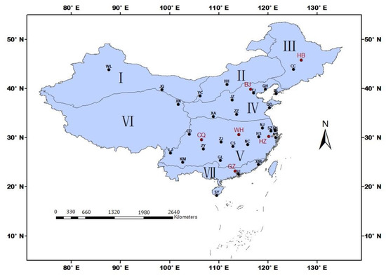
Figure 1.
Distribution of the large tourist cities in this study. The cities with red color are used for exploring optimal methods on solar radiation estimation, and the cities with black color are the other tourism cities in this study. Roman numerals indicate the climate zones in China. I denotes the temperate and warm-temperate deserts of northwest China, II Inner Mongolia, III the temperate humid and sub-humid northeastern China, IV the temperate humid and sub-humid northern China, V the subtropical humid central and southern China, VI the Qinghai–Tibetan Plateau, and VII the tropical humid southern China. Whole names of the cities can be seen in Table 1.

Table 1.
Detailed information of the tourism cities in China.
For this research, access to the fundamental database of NMIC (National Meteorological Information Center) was given by CMA (China Meteorological Administration). The daily meteorological data, including sunshine hours, mean temperature, maximum temperature, minimum temperature, vapor pressure, relative humidity, wind speed, precipitation, and cloudiness, were collected from 1961 to 2020 for all of these locations. There were very few missing values in the dataset. When a missing value was identified, it was substituted by the average of the values observed on preceding and following days [10]. Solar radiation is not a routinely observed meteorological item in most weather stations in China, and the daily solar radiation data were only available in six stations, i.e., Harbin, Beijing, Wuhan, Chongqing, Hangzhou, and Guangzhou. Daily solar radiation data from 1991 to 2020 in these locations were believed to be reliable after strict data quality control made by NMIC, so the datasets from 1991 to 2010 were used for model calibration, while the datasets from 2011 to 2020 were used for model validation in this study.
2.2. Calculation of UTCI
UTCI is defined as the isothermal air temperature which would elicit the same response under a set of reference conditions [7]. UTCI is calculated by solving Fiala’s heat balance model [3], which calculates the human physical response to meteorological conditions. The model is based on a thermoregulation model, consisting of 12 human body elements and 187 tissue nodes [3]. A rapid calculation of UTCI can be achieved by a polynomial approximation procedure to compute the offset of UTCI to Ta (UTCI−Ta) as follows [16].
where Ta denotes the air temperature, V the wind speed, e the vapor pressure, and Tmrt the mean radiative temperature, respectively. V, e, and Tmrt can be computed as:
where Vu and Vv are wind speed at meridional and longitudinal directions, respectively; Td is the dew point temperature, Tg is the ground temperature, and Rp is the solar radiation observed by a nude man, which can be estimated by the SolAlt model [9,44].
UTCI is divided into 10 categories ranging from extreme cold stress to extreme heat stress [16] (Table 2). This category has been extensively validated by both climate chamber and wind tunnel experiments [3,19], and widely accepted by both the International Society on Biometeorology [3,7,16] and the researchers in this domain [21,22,23,24,25,26]. Currently, calculation of UTCI can be performed by Bioklima 2.6 software package with four meteorological input variables, including solar radiation, air temperature, vapor pressure or humidity, and wind speed [9,23]. Detailed description on the input variables can be found in the relevant procedures and processing steps [44].

Table 2.
Category for UTCI in terms of thermal stress (according to Brode et al. [16]).
2.3. Estimation of Solar Radiation
Two sunshine- and two temperature-based empirical models, together with two machine-learning methods, were used to estimate solar radiation in this study.
2.3.1. Angstrom Model
The Angstrom formula is the most widely used popular empirical sunshine-based model [46,47], which calculates solar radiation with sunshine hours as follows.
where Ra is the observed daily solar radiation, Re the extra-terrestrial solar radiation, S the observed sunshine hours, and S0 the potential sunshine hours, respectively. Re and S0 can be calculated with the method recommended by FAO [48].
2.3.2. Ogelman Model
The Ogelman model is also an empirical sunshine-based model, which can be expressed as [49]
2.3.3. Bristow Model
The Bristow model is an empirical temperature-based model, using temperature as input variables to predict solar radiation [50].
where is the difference between daily maximum and minimum temperature.
2.3.4. Hargreaves Model
The Hargreaves model is also an empirical temperature-based model, estimating solar radiation with the diurnal range of temperature [51].
2.3.5. BP Neural Network
BP neural network has one or more hidden layers, and one output layer. The data are propagated from input layer to output layer through hidden layer with error being transmitted in the opposite direction, so the connection weight of the network can be corrected to decrease the final error. Recently, BP neural has been argued to be efficient in solar radiation estimation [52].
2.3.6. Support Vector Machine
The support vector machine (SVM) is a supervised machine-learning method for data analysis and pattern recognition. The SVM follows the concept of separating the features from one another. According to the algorithm of SVM, the same types of features are set on one plane. To be specific, the SVM aims to find a hyperplane that can separate data points of one class from another to the best degree. The best degree is referred to as the hyperplane with the largest margin between the two classes, and margin is defined as the biggest width of the slab parallel to the hyperplane that has no interior data points. Based on the principle of structural risk minimization, this method can better solve the problems with nonlinearity and high dimensionality. Up to now, SVM has been widely employed for radiation estimation due to its high accuracy [41].
2.4. Statistical Analysis
The Nash–Sutcliffe Efficiency (NSE), the Mean Absolute Percentage Error (MAPE), and the Root Mean Square Error (RMSE) were used as criteria to evaluate the model performance [39,53]. NSE is analogous to coefficient of determination, with the exception that NSE ranges from negative infinity to 1, which can be used for indicating model efficiency. The negative value of NSE indicates that the mean observation can be used as a better predictor than the simulated values. MAPE is used to identify the relative bias in simulated values compared with observations, while RMSE is an indicator of the squared difference between simulated and measured values.
where Oi is the observed value, Si the estimated value, the average of the observed value, and n the sample number of observations, respectively. Higher NSE and lower MAPE and RMSE mean better model performance.
Trends in time series of UTCI were estimated by the nonparametric Theil–Sen’s estimator [54].
where Xi and Xj are the UTCI values for year i and j, respectively. Positive β denotes an increase in trend, while negative value of β indicates decrease in the time series. The trend significance was tested by Mann–Kendall method. Detailed information on calculating the standardized test statistic (z) of MK can be referred to the relevant descriptions [10,55,56].
The empirical coefficients of a, b and c in Equations (7)–(10) were fitted by numerical iteration methods [53]. The BP and SVM methods were implemented through the “nnet” and “e1071” packages in R language, respectively. A regression task was involved in the study, and both the empirical models and the machine-learning methods were calibrated and validated before application. The machine-learning methods are believed to be more accurate in radiation estimation than the empirical models [41], but they require big data for model training. In contrast, the empirical models are easy to operate, and require less data for model calibration than the machine-learning methods.
3. Results
3.1. Comparison of Model Performance in Radiation Estimation and UTCI Calculation
Coefficients of the empirical models were calibrated with the dataset from 1991 to 2010, and the calibration results are shown in Table 3. For the sunshine-based Angstrom model, the coefficient a ranged from 0.130 to 0.240 with averaged value of 0.16, while the coefficient b ranged from 0.456 to 0.587 with an average of 0.528. The values of NSE were between 0.861 and 0.930 with an average of 0.886, indicating that Angstrom had a high efficiency in radiation estimation. The average MAPE and RMSE were 16.795 and 27.452, respectively. The calibration performance of the Ogelman model was very similar to that of the Angstrom model. The average NSE was 0.895 for the Ogelman model, which was almost equal to that of the Angstrom model. In addition, the values of MAPE and RMSE were also very close to those of the Angstrom model, either for each location or as a whole. For temperature-based models, the average value of NSE was 0.673 for the Bristow model, and the average values of MAPE and RMSE were 22.94 and 46.386, respectively. The Hargreaves model showed a similar performance as the Bristow model with very close NSE, MAPE, and RMSE values.

Table 3.
Calibration results of the empirical models and machine-learning methods on estimation of the solar radiation.
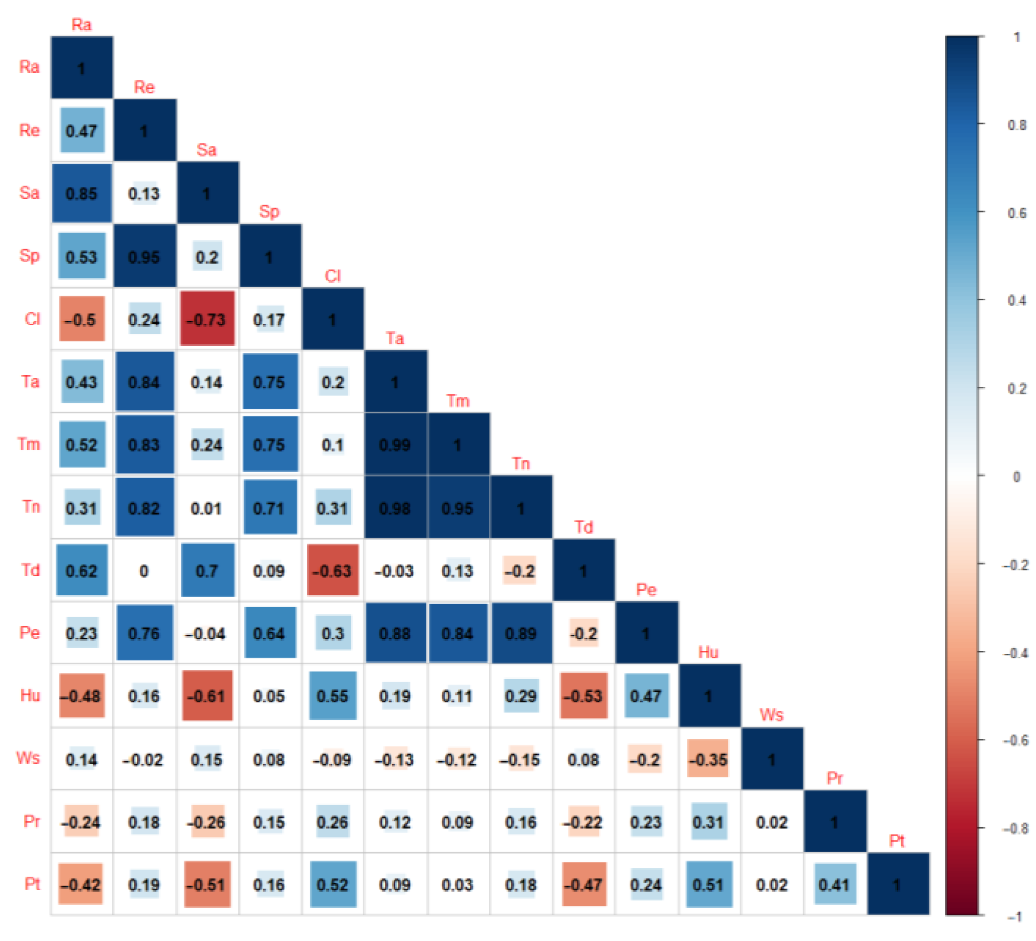
Correlation analysis identified that many meteorological factors should be used as input variables for training machine leaning methods, including extra-terrestrial solar radiation (Re), sunshine hours (Sa), potential sunshine hours (Sp), cloudiness (Cl), air mean temperature (Ta), maximum temperature (Tm), minimum temperature (Tn), diurnal variation of temperature (Td), vapor pressure (Pe), humidity (Hu), wind seep (Ws), precipitation (Pr), and precipitation events (Pt) (Figure 2). However, the machine-learning models could be over-trained when the highly correlated features were used as input variables simultaneously. In this study, when the correlation coefficients among several features were higher than 0.8, only one feature was used as the input variable for the machine-learning models. According to this rule, together with the consideration of the data availability, Ta was kept as input variable for machine-learning models, while Tm, Tn, and Pe were removed from the dataset. However, all of the three sunshine-related features, including Sp, Re, and Sa, were used as input variables despite of their high correlation coefficients, as removal of any one of these features would lead to poor performance of the machine-learning models. The machine-learning models were also trained with the dataset from 1991 to 2011 for comparison with the results by the empirical models (Table 3). A “Trial and error” method was used to tune the machine-learning models to determine the best parameters. For the BP model, the number of units in the hidden layer and the parameter for weight decay were set as 10 and 0.01, respectively. For the SVM model, the kernel used in training and predicting was set as “radial” basis, and the cost of constraints violation was tuned as 1. The value of gamma was determined as 0.125. The two machine-learning methods performed better in calibration with higher NSE and lower MAPE and RMSE. The average values of NSE, MAPE, and RMSE were 0.938, 14.210, and 20.127, respectively, for the BP neural network, while the Support Vector Machine further improved the model performance in calibration by a slightly higher NSE of 0.940, and lower MAPE and RMSE of 13.711 and 19.781, respectively.

Figure 2.
Correlations among different meteorological items.
The calibrated empirical models and trained machine-learning models were used for validation against the observed radiation from 2011 to 2020, respectively. The validation results are shown in Table 4. For each empirical model, the overall model performance in validation was quite similar to that in calibration. However, compared to the performance in calibration, the machine-learning methods showed worse performance in validation. The average value of NSE was 0.878 for the BP neural network, much lower than that of 0.938 in calibration. In addition, the values of MAPE and RMSE also became larger in model validation for machine-learning methods.

Table 4.
Validation results of the empirical models and machine-learning methods on estimating solar radiation.
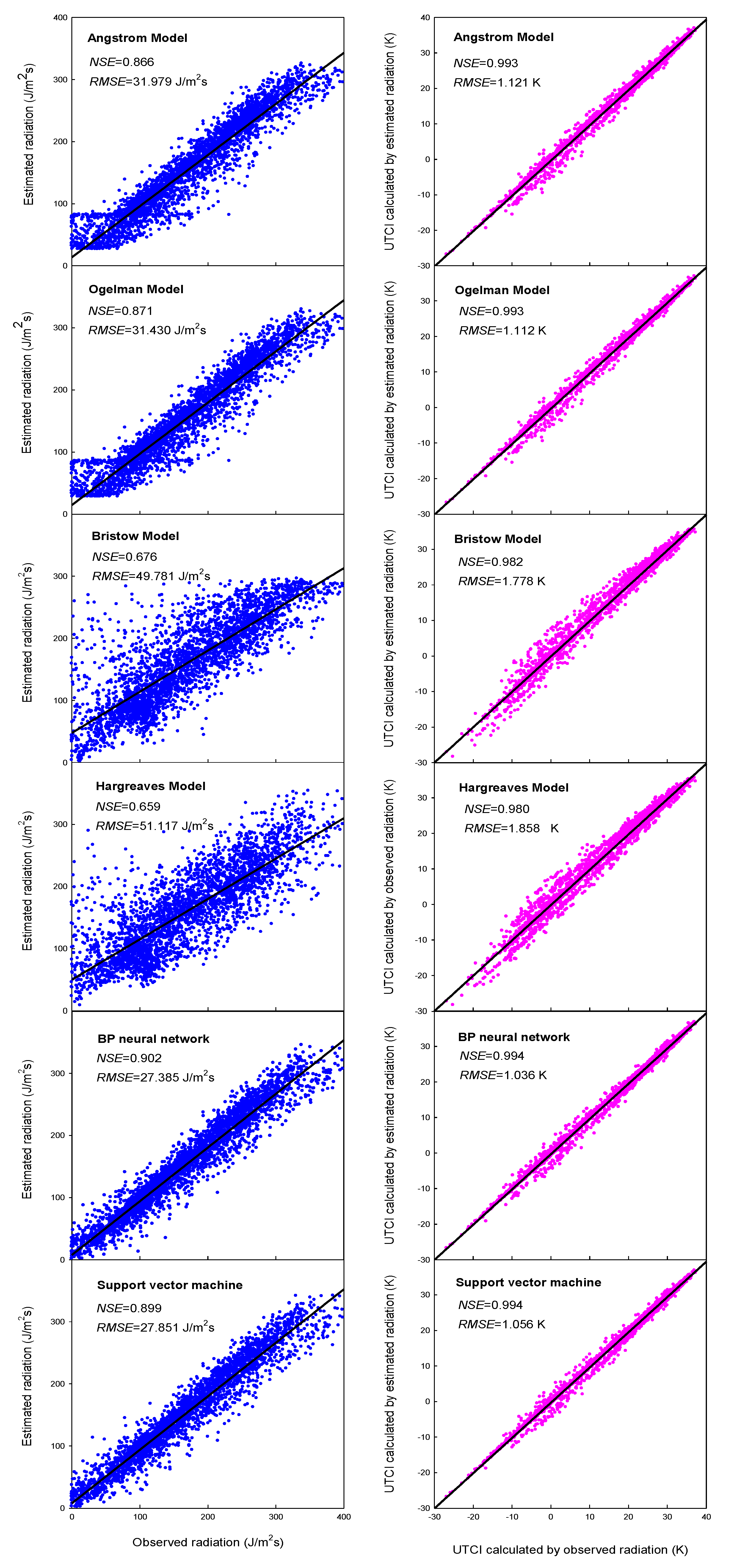
The estimated radiation dataset in 2011–2020 was used to calculate UTCI, and the obtained UTCI was compared to that calculated with observed radiation. The UTCI validation result is shown in Table 5. As a whole, the error in radiation estimation was not amplified, but reduced in the UTCI calculation process. The sunshine-based Angstrom model had a high average NSE value of 0.990, and lower RMSE value of 1.236 (Table 5). Referred to the validation in radiation (Table 4), an average error of 35.4 J/m2 s radiation estimation led to an average error of 1.2 °C in UTCI calculation, which was exactly within the error range of 2.1 °C identified by sensitivity analysis [4]. The Ogelman model showed very similar performance to the Angstrom model. However, the temperature-based models, both the Bristow and Hargreaves models, presented lower NSE and higher MAPE and RMSE than sunshine-based models. In contrast, the NSE values of the machine-learning methods were 0.992, slightly higher than those of the sunshine-based models. The average RMSE value for both machine-learning methods was about 1.1 °C, showing very limited advantage over the sunshine-based models. Considering both accuracy and applicability, the Angstrom model was selected to estimate solar radiation for UTCI calculation in regional analysis below, due to its easy calibration and readily available input data. The accuracy of the Angstrom model in calculating UTCI and day number within each category can be seen in Figure 3 and Figure 4, respectively.

Table 5.
Validation results of the UTCI calculation based on solar radiation estimated by empirical models and machine-learning methods.

Figure 3.
Validation of the radiation estimation and UTCI calculation in Beijing by different methods.
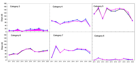
Figure 4.
Comparison of the days within each UTCI category calculated by observed radiation (line blue circle) with those by estimated radiation (line with pink triangle).
3.2. Spatial Analysis of UTCI and Day Number within Each Category
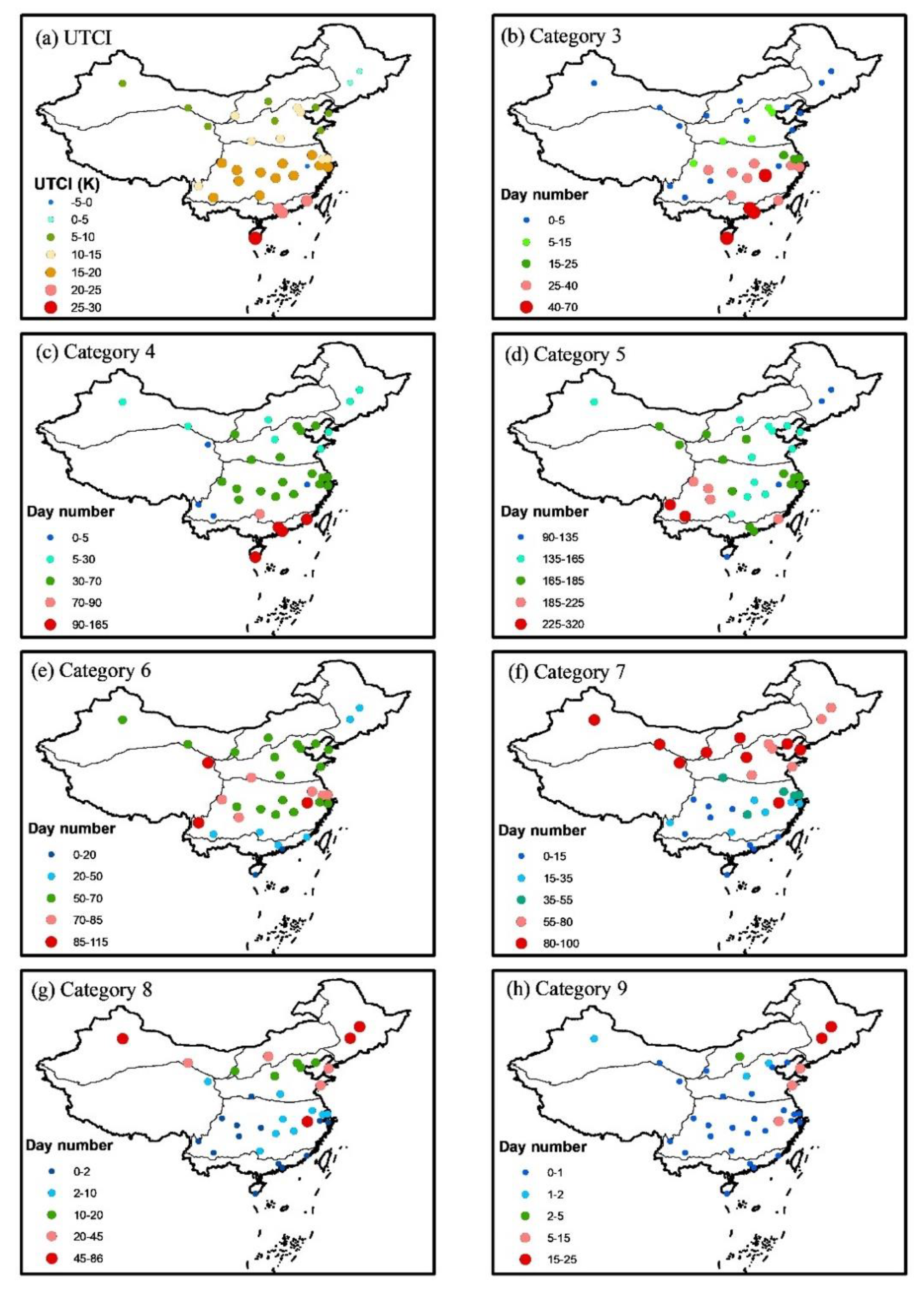
The calibrated model was used to calculate the UTCI in all of the tourism cities from 1961 to 2020. The spatial distribution of average yearly UTCI and the days within each category in Chinese tourism cities are shown in Figure 5a, and the detailed information is shown in Table 6. As a whole, the UTCI increased gradually from north to south in the tourism cities of China, with the exception of Huangshan location due to its high altitude (see Table 1). UTCI in the tourism cities of northeast China was lower than 5 °C, while the UTCI reached the highest value around 28 °C in Sanya, the southernmost part of China. The days within each category are shown in Figure 5b–h. For the days under no thermal stress (Figure 5d), Kunming and Lijiang had the largest value between 225 and 320 days. The tourism cities in northeast and southeast China had the lowest values between 90 and 135 days with the lowest and highest UTCI, respectively. The tourism cities in the most developed regions such as the Yangtze River Delta and Zhujiang River Delta had about 170 days under no thermal stress in a year. The distribution of days under slightly cold stress was very similar to that under no thermal stress (Figure 5e).
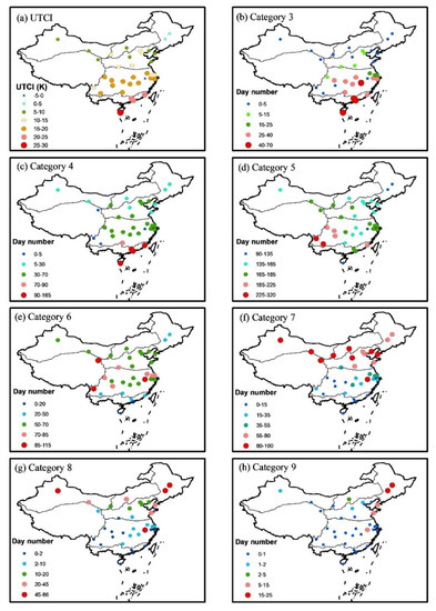
Figure 5.
Spatial distribution of UTCI and yearly days within each category in the large tourism cities of China.

Table 6.
Detailed information on UTCI and the yearly days within each category in the large tourism cities of China.
In contrast with the spatial distribution of days under no thermal stress and slightly cold stress, more days under heat stress were identified in the tourism cities of south China (Figure 5b,c), while more days under cold stress were found in the tourism cities of north China (Figure 5f–h). According to category 3, many tourism cities in the lower reach of Yangtze River, including Wuhan, Nanjing, Hangzhou, and Shanghai etc., had about one month under strong heat stress, while the tourism cities in Zhujiang River Delta such as Guangzhou and Shenzhen had about two months under strong heat stress in a year. Sanya, the southernmost China, experienced 70 days under strong heat stress in a year.
Strong cold stress mainly occurred in the tourism cities of north China. The largest days under strong cold stress occurred in Harbin and Changchun in northeast China and Wulumuqi in northwest China, in a range from 45 to 86 days in a year (Figure 5g). Days under very strong cold stress occurred very seldom in most tourism cities of China. Many locations, 28 out of 35 cities, had less than two days under very strong cold stress, most of which were located in south China (Figure 5h). However, Changchun and Harbin in northeast China did experience very strong cold stress in a year with day number between 15 and 25.
3.3. Temporal Trend in UTCI and Day Number within Each Category
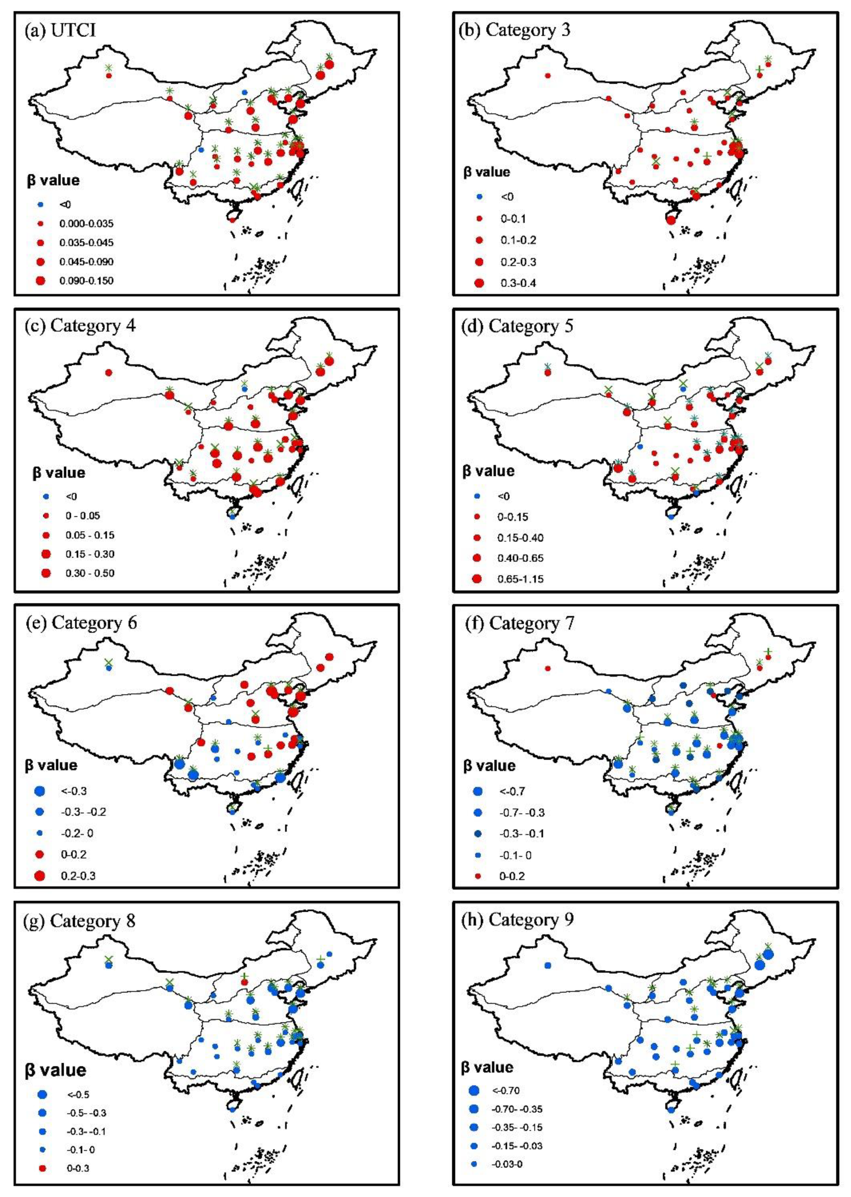
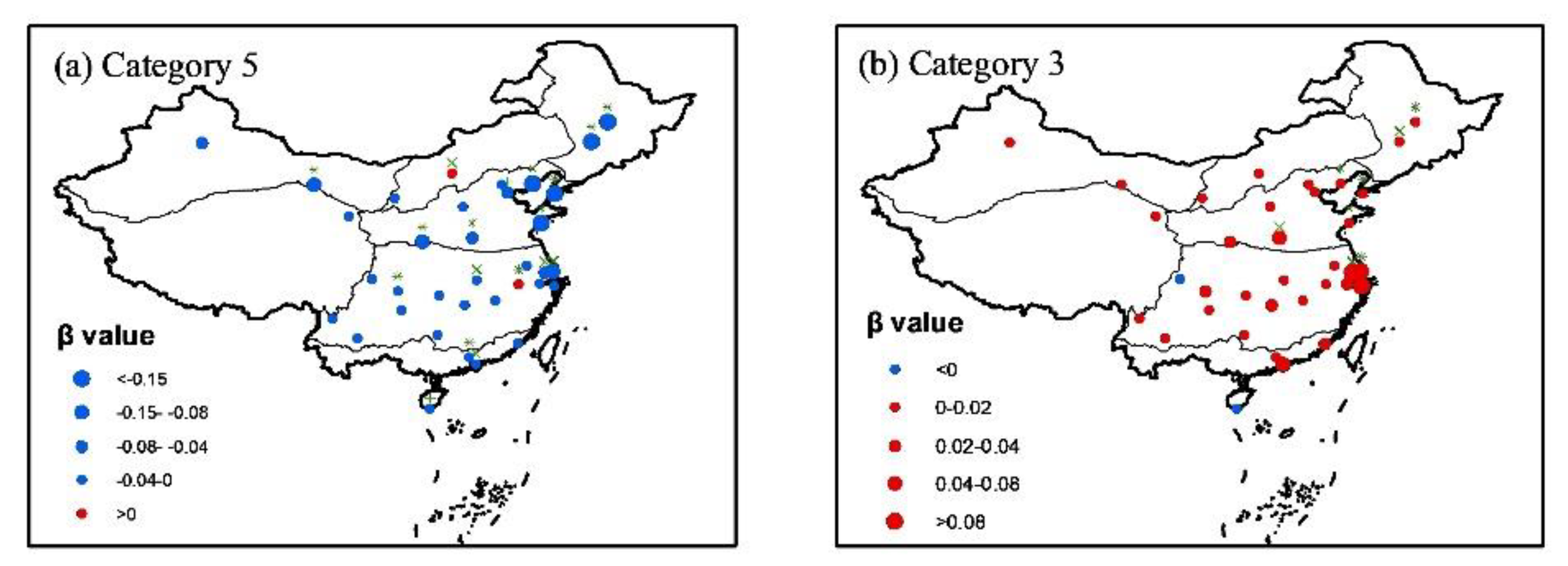
The time analysis was further conducted with the calculated UTCI in all of the tourism cities from 1961 to 2020, and the trend analysis of the UTCI and days number within each category from 1961 to 2020 is presented in Figure 6. On the whole, the UTCI showed an overall increasing trend for most of the large tourism cities in China (Figure 6a), most of which increased with very high statistical significance level of 99% (z > 2.58). Only 2 out of 35 tourism cities showed negative trends in UTCI. Huhehaote had a negative trend with very small value of −0.009 °C/a, and the negative trend in UTCI was negligible in Chengdu with an even smaller value of −0.001 °C/a. In addition, both trends did not pass the significant level of 90% (z < 1.96). In other words, very slight decreases in both locations were not significant in terms of statistical analysis. Generally speaking, the days under no thermal stress increased in most of the tourism cities over China (Figure 6d). The days under slight cold stress increased in most locations in the northern parts of China, while they decreased in most locations in the southern parts of China (Figure 6e). The days under moderate heat stress and strong heat stress generally increased over China from 1961 to 2000 (Figure 6b,c). In contrast with these increasing trends, trends in the days under moderate cold, strong cold, and very strong cold stresses presented an overall decreasing trend in most locations over China (Figure 6f–h). Especially, the days under very strong cold stress decreased in all locations of China (Figure 6h). In short, the UTCI increased in most locations of China, accompanying with an overall increase in days under no thermal stress and heat stress, and an overall decrease in days under cold stress (Figure 6a–h).
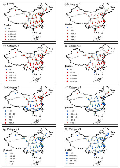
Figure 6.
Trend analysis of the changes in yearly day number within each category from 1961 to 2020. Plus +, multiple ×, and asterisk * signs denote confidence levels of 90%, 95%, and 99%, respectively.
4. Discussion
4.1. Optimal Strategy on Estimating Solar Radiation for UTCI Calculation
The sunshine-based Angstrom model was selected as the best choice to estimate solar radiation for UTCI calculation. In this study, the sunshine-based models performed better than the temperature-based models in terms of higher NSE and lower MAPE and RMSE (Table 3 and Table 4), which was in agreement with the results from the previous reports [33,38]. The machine-learning method is believed to be a promising choice for accurate estimation of solar radiation [41], but the strict requirement of many input variables for model training cannot always be met, which inevitably leads to better performance in calibration but worse performance in validation [57]. This inherent defect was again identified by the higher NSE in calibration and the lower NSE in validation in this study (Table 3 and Table 4). In fact, the machine-learning methods can only slightly improve the accuracy in radiation estimation compared with the sunshine-based models, but require many more input variables and datasets for model training [41]. Due to limitation of length, only the BP and SVM methods were implemented in this study. Recently, the Random Forest method has also been identified as an effective algorithm in radiation estimation [58], which may outperform the BP and SVM methods. So, involvement of more machine-learning methods to further improve accuracy in radiation estimation becomes necessary in the future research work.
Based on sensitivity analysis, Weihs et al. [4] concluded that the maximum uncertainty in solar radiation estimation would be 15% in conventional sites, which might contribute to a maximum uncertainty in UTCI with 2.1 °C. In this study, the RMSE of the radiation by the Angstrom model was 32 J/m2 s in Beijing, while the average solar radiation was around 300 J/m2 s in clear days (Figure 3). This error resulted in an uncertainty of about 11% in radiation estimation, which further led to an uncertainty of about 1.2 °C in UTCI calculation (Figure 3), just within the error range made by sensitivity analysis [4]. Therefore, it can be reasonably concluded that accurate UTCI can be obtained through the optimal strategy for radiation estimation. Based on the results and analysis above, the sunshine-based Angstrom model is recommended as the optimal strategy due to its excellent model performance, easy operation, and readily available input variables.
4.2. Increase in Yearly Day Number under no Thermal Stress Accompanying with More Risks in Heat Stress in Summer in China
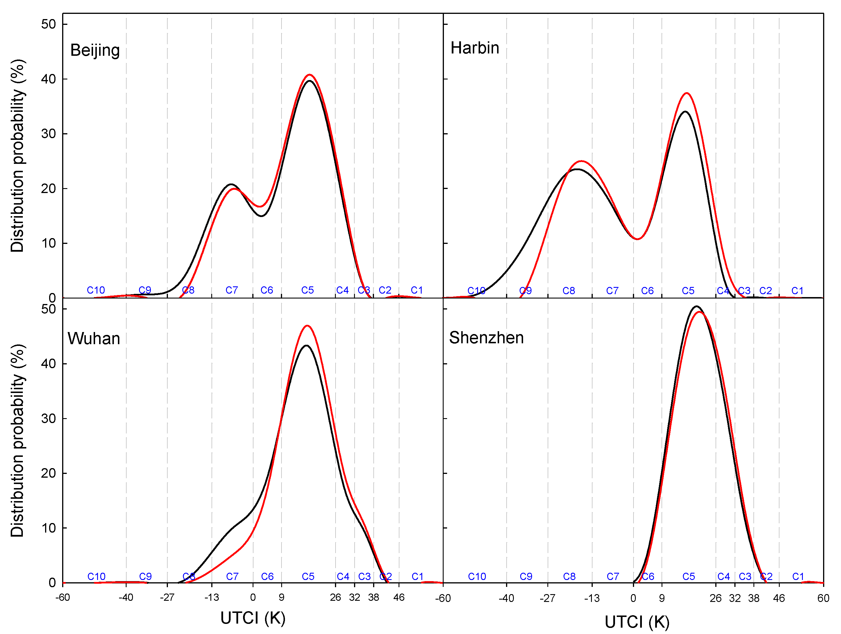
Global warming has been well acknowledged in modern society [59], with its great negative effects in many aspects such as the economy [60], agriculture [61], and global food security [62]. In addition, climate change is also believed to give rise to more extreme weather events, which would pose great risks to the public health [63,64,65,66,67]. Considering so many impressive negative impacts, people would naturally envisage that days under no thermal stress would decrease in the context of climate change. However, this study showed an opposite result in that the yearly day number under no thermal stress increased in most tourism cities over China in the recent six decades (Figure 6d). To investigate its reliability, the probability of days under each category in the period of 1961–1990 and 1991–2020 was analyzed, respectively. Figure 7 clearly indicates that the distribution probability curve slightly right-shifted in the tourism cities of China. This shift can be attributed to the decrease in cold days and increase in warm days caused by climate warming. For most locations, more days under cold stress changed to the days under no thermal stress, while fewer days under no thermal stress shifted to the days under heat stress. This might be the exact reason for the increasing days under no thermal stress in most tourism cities of China. Only for very few tourism cities such as Shenzhen was this shift was not significant due to the high temperature in south part of the tropical humid zone. In short, it is the asymmetric changes in the hot days and cold days that led to the increase in days under no thermal stress within a year in the tourism cities of China. This argument is strongly justified by the previous report given by Zhai et al. [68], who identified that the number of hot days displayed a slight increasing trend, while the number of the frost days exhibited a significant decreasing trend in China in the recent decades.
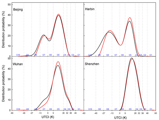
Figure 7.
Distribution probability of the days within each category in the period of 1961–1990 (black lines) and 1991–2020 (red lines).
The increase in days under no thermal stress mainly occurred in the spring and autumn. In summer, the days under no thermal stress did decease (Figure 8a). Without consideration of the radiation effect on UTCI, Yan et al. [10] also believed that days under no thermal stress have been decreasing in most locations of China from 1961 to 2016 in summer. In contrast to the decrease in days under no thermal stress, the days under strong heat stress showed an increasing trend in most tourism cities in summer (Figure 8b), which would inevitably cause more potential heat threats to the public health and make the further investigation on thermal perception essential and urgent [28].

Figure 8.
Trend analysis of the changes in day number under no thermal tress (a) and strong heat stress (b) in summer from 1961 to 2020.
4.3. Certainties and Uncertainties in UTCI Estimation over China
It is certain that UTCI deserves its name, as the term “universal” means that UTCI is appropriate for all assessments of the outdoor thermal conditions in the major human bio-meteorological applications [7]. Previously, many simple thermal indices have already been suggested in different regions in China [69,70,71], but none of them could be used for the spatial analysis at the national scale over China due to regional adaptability. In contrast, UTCI successfully revealed the overall distribution of the thermal environments in the tourism cities of China (Figure 5), and the results are highly consistent with public cognition. For example, Kunming is called “spring city” due to its long period of thermal comfort, which has been identified by UTCI as the city with the most days under no thermal stress (Figure 5d). The general distribution of more cold stress in tourism cities of north China and more heat stress in tourism cities of south China also agree well with the basic public cognition. However, it should be noted that Huangshan is an exception of this the general spatial distribution of UTCI (Figure 5a). Though located in the central part of China, the yearly UTCI of Huangshan is much lower than the surrounding cities due to its high altitude (Table 1). This unique UTCI makes Huangshan become one of the most attractive tourism destinations in the summertime. So, the effect of topographic features on UTCI should be explored in the future research relevant to the distribution of thermal environments in China.
The general spatial distribution of UTCI in the tourism cities of China is comparable to the previous reports [9,44], with quantitative differences due to different strategies on dealing with input variables. In the future, error in UTCI calculation caused by using cloudiness [9] or simple interpolation [44] should be examined deliberately. In addition, UTCI stress should be redefined at daily scale. Currently, UTCI category is defined at hourly scale [16]. However, air temperature has obvious seasonal and daily changes, especially in the monsoon climate regions such as China [72]. As air temperature is the dominant element of UTCI, and UTCI also has seasonal and daily changes at daily and seasonal scales. Therefore, both heat stress and cold stress would be underestimated if the daily UTCI were classified according to the current UTCI category at the hourly scale. For example, the daily UTCI of 26 °C was defined as no thermal stress (9–26 °C) according to the current hourly category (Table 2). However, there is a great possibility that UTCI is higher than 26 °C in many hours during the day, so it actually should be classified as moderate heat stress rather than no thermal stress in this day. Vice versa, the daily UTCI of 9 °C should actually be referred to as a slight cold day, as UTCI would be lower than 9 °C in many hours of the day. Likewise, daily UTCI values within category 3 or category 9 might actually belong to category 2 or category 10. This might be the exact reason that no very strong heat stress (category 10) and extreme hot stress (category 2) were identified in both this study and all of the previous reports, which is obviously contradicted to the public cognition that there are many “ice” and “furnace” cities in China. Thus, it is urgent to redefine UTCI category at daily scale through comparison of daily UTCI with hourly values in the future work.
5. Conclusions
The sunshine-based Angstrom model performed well in estimation of solar radiation in the tourism cities of China with high NSE of 0.864 and low RMSE of 35.4, which resulted in a high efficiency in UTCI calculation with NSE of 0.99. Uncertainty in UTCI calculation with estimated solar radiation by the Angstrom model was 1.2 °C, just within the error range obtained by sensitivity analysis. So, the Angstrom model is proposed as the optimal strategy on solar radiation estimation for UTCI calculation due to its high accuracy and easy operation.
Spatial distribution of UTCI indicated that day number under no thermal stress was higher in the tourism cities of central China, within a range from 135 to 225 days, and the largest days under no thermal stress occurred in Kunming and Lijiang in southwest China. Very strong cold stress mainly occurred in Harbin and Changchun in northeast China, with a period between 15 and 25 days in a year. Strong heat stress mainly occurred in the tourism cities of south China, especially southernmost Sayan, with a period between 40 and 70 days in a year.
Contrary to popular belief, days under no thermal stress during a year have increased in most tourism cities of China in the recent decades in the context of global warming, which can be attributed to the asymmetric changes in the significant decrease in frost days and slightly increase in hot days over China in the recent decades. However, in the summer, days under no thermal stress have decreased in most regions of China, accompanying with increasing trends in days under very strong heat stress, especially in the developed regions such as Yangtze River Delta and Zhujiang River Delta, which would pose great risks to thermal perception for the public health in these regions.
UTCI can successfully identify the general spatial distribution and temporal trend of thermal environments in most tourism cities of China. However, up to now, all reports on Chinese UTCI were performed by classifying daily UTCI values according to the category obtained at hourly scales, which would result in the underestimation of days under extreme hot or cold stress conditions. This is exactly the weakness of UTCI performance in China, i.e., no extreme cold or extreme hot days have been identified by the daily UTCI values. Thus, it is urgent to redefine UTCI category at daily scales by comparing daily UTCI with the corresponding hourly values in the future research work.
Author Contributions
Conceptualization, J.L., D.-L.L. and G.Z.; methodology, J.L.; Y.S. (Yanling Song); software, J.L.; validation, Y.L., J.D. and Y.S. (Yanbo Shen), D.-L.L. and G.Z.; formal analysis, J.L.; writing—original draft preparation, J.L.; writing—review and editing, D.-L.L. and H.W.L. All authors have read and agreed to the published version of the manuscript.
Funding
This research was supported by the National Key R&D Program of China, under the grant No. 2018YFB1500901, and the Second Tibetan Plateau Comprehensive Research Project (2019QZKK0106).
Institutional Review Board Statement
Not applicable.
Informed Consent Statement
Not applicable.
Data Availability Statement
Not applicable.
Acknowledgments
Special thanks to Yechao Yan and Shuangshuang Li for their useful discussions on the application of UTCI model in the public health services in China.
Conflicts of Interest
The authors declare no conflict of interest.
References
- Jendritzky, G.; Nübler, W. A model analyzing the urban thermal environment in physiologically significant terms. Arch. Meteorol. Geophys. Bioclim. 1981, 29, 313–326. [Google Scholar] [CrossRef]
- Fröhlich, D.; Matzarakis, A. A quantitative sensitivity analysis on the behavior of common thermal indices under hot and windy conditions in Doha, Qatar. Theor. Appl. Climatol. 2016, 124, 179–187. [Google Scholar] [CrossRef]
- Fiala, D.; Havenith, G.; Bröde, P.; Kampmann, B.; Jendritzky, G. UTCI-Fiala multi-node model of human heat transfer and temperature regulation. Int. J. Biometeorol. 2012, 56, 429–441. [Google Scholar] [CrossRef] [Green Version]
- Weihs, P.; Staiger, H.; Tinz, B.; Batchvarova, E.; Rieder, H.; Vuilleumier, L.; Jendritzky, G. The uncertainty of UTCI due to uncertainties in the determination of radiation fluxes derived from measured and observed meteorological data. Int. J. Biometeorol. 2012, 56, 537–555. [Google Scholar] [CrossRef]
- Thorsson, S.; Lindberg, F.; Eliasson, I.; Holmer, B. Different methods for estimating the mean radiant temperature in an outdoor urban setting. Int. J. Climatol. 2007, 27, 1983–1993. [Google Scholar] [CrossRef]
- Matzarakis, A.; Rutz, F.; Mayer, H. Modelling radiation fluxes in simple and complex environments: Basics of the RayMan model. Int. J. Biometeorol. 2010, 54, 131–139. [Google Scholar] [CrossRef] [Green Version]
- Jendritzky, G.; de Dear, R.; Havenith, G. UTCI—why another thermal index? Int. J. Biometeorol. 2012, 56, 421–428. [Google Scholar] [CrossRef] [PubMed] [Green Version]
- Matzarakis, A. Weather-and climate-related information for tourism. Tour. Hosp. Plan. Dev. 2006, 3, 99–115. [Google Scholar] [CrossRef]
- Ge, Q.; Kong, Q.; Xi, J.; Zheng, J. Application of UTCI in China from tourism perspective. Theor. Appl. Climatol. 2017, 128, 551–561. [Google Scholar] [CrossRef]
- Yan, Y.; Wang, D.; Yue, S.; Qu, J. Trends in summer air temperature and vapor pressure and their impacts on thermal comfort in China. Theor. Appl. Climatol. 2019, 138, 1445–1456. [Google Scholar] [CrossRef]
- Houghten, F.C. Determining lines of equal comfort. ASHVE Trans. 1923, 29, 163–176. [Google Scholar]
- Siple, P.A.; Passel, C.F. Measurements of dry atmospheric cooling in subfreezing temperatures. Proc. Am. Philos. Soc. 1945, 89, 177–199. [Google Scholar] [CrossRef]
- Thom, E.C. The discomfort index. Weatherwise 1959, 12, 57–61. [Google Scholar] [CrossRef]
- Matzarakis, A.; Rutz, F.; Mayer, H. Modelling radiation fluxes in simple and complex environments—Application of the RayMan model. Int. J. Biometeorol. 2007, 51, 323–334. [Google Scholar] [CrossRef]
- Błazejczyk, K. New climatological and physiological model of the Human Heat Balance outdoor (MENEX) and its applications in bioclimatological studies in different scales. Zeszyty Instytutu Geografii i Przestrzennego Zagospodarowania PAN 1994, 28, 27–58. [Google Scholar]
- Bröde, P.; Fiala, D.; Błażejczyk, K.; Holmér, I.; Jendritzky, G.; Kampmann, B.; Havenith, G. Deriving the operational procedure for the Universal Thermal Climate Index (UTCI). Int. J. Biometeorol. 2012, 56, 481–494. [Google Scholar] [CrossRef] [Green Version]
- Fiala, D.; Lomas, K.J.; Stohrer, M. A computer model of human thermoregulation for a wide range of environmental conditions: The passive system. J. Appl. Physiol. 1999, 87, 1957–1972. [Google Scholar] [CrossRef]
- Fiala, D.; Lomas, K.J.; Stohrer, M. Computer prediction of human thermoregulatory and temperature responses to a wide range of environmental conditions. Int. J. Biometeorol. 2001, 45, 143–159. [Google Scholar] [CrossRef]
- Kampmann, B.; Bröde, P.; Fiala, D. Physiological responses to temperature and humidity compared to the assessment by UTCI, WGBT and PHS. Int. J. Biometeorol. 2012, 56, 505–513. [Google Scholar] [CrossRef]
- Blazejczyk, K.; Epstein, Y.; Jendritzky, G.; Staiger, H.; Tinz, B. Comparison of UTCI to selected thermal indices. Int. J. Biometeorol. 2012, 56, 515–535. [Google Scholar] [CrossRef] [Green Version]
- Roshan, G.; Nastos, P.T. Assessment of extreme heat stress probabilities in Iran’s urban settlements, using first order Markov chain model. Sustain. Cities. Soc. 2018, 36, 302–310. [Google Scholar] [CrossRef]
- Di Napoli, C.; Pappenberger, F.; Cloke, H.L. Assessing heat-related health risk in Europe via the Universal Thermal Climate Index (UTCI). Int. J. Biometeorol. 2018, 62, 1155–1165. [Google Scholar] [CrossRef] [Green Version]
- Zare, S.; Hasheminejad, N.; Shirvan, H.E.; Hemmatjo, R.; Sarebanzadeh, K.; Ahmadi, S. Comparing Universal Thermal Climate Index (UTCI) with selected thermal indices environmental parameters during 12 months of the year. Weather. Clim. Extreme. 2018, 19, 49–57. [Google Scholar] [CrossRef]
- Vinogradova, V. Using the Universal Thermal Climate Index (UTCI) for the assessment of bioclimatic conditions in Russia. Int. J. Biometeorol. 2021, 65, 1473–1483. [Google Scholar] [CrossRef]
- Pecelj, M.M.; Lukić, M.Z.; Filipović, D.J.; Protić, B.M.; Bogdanović, U.M. Analysis of the Universal Thermal Climate Index during heat waves in Serbia. Nat. Hazard Earth Sys. 2020, 20, 2021–2036. [Google Scholar] [CrossRef]
- Pantavou, K.; Lykoudis, S.; Nikolopoulou, M.; Tsiros, I.X. Thermal sensation and climate: A comparison of UTCI and PET thresholds in different climates. Int. J. Biometeorol. 2018, 62, 1695–1708. [Google Scholar] [CrossRef]
- Leroyer, S.; Bélair, S.; Spacek, L.; Gultepe, I. Modelling of radiation-based thermal stress indicators for urban numerical weather prediction. Urban. Clim. 2018, 25, 64–81. [Google Scholar] [CrossRef]
- Kong, Q.; Ge, Q.; Xi, J.; Zheng, J. Human-biometeorological assessment of increasing summertime extreme heat events in Shanghai, China during 1973–2015. Theor. Appl. Climatol. 2017, 130, 1055–1064. [Google Scholar] [CrossRef]
- Morcrette, J.J.; Mozdzynski, G.; Leutbecher, M. A reduced radiation grid for the ECMWF Integrated Forecasting System. Mon. Weather Rev. 2008, 136, 4760–4772. [Google Scholar] [CrossRef]
- Manners, J.; Thelen, J.C.; Petch, J.; Hill, P.; Edwards, J.M. Two fast radiative transfer methods to improve the temporal sampling of clouds in numerical weather prediction and climate models. Q. J. R. Meteor. Soc. 2009, 135, 457–468. [Google Scholar] [CrossRef]
- Janjai, S.; Pankaew, P.; Laksanaboonsong, J. A model for calculating hourly global solar radiation from satellite data in the tropics. Appl. Energy 2009, 86, 1450–1457. [Google Scholar] [CrossRef]
- Pinker, R.T.; Frouin, R.; Li, Z. A review of satellite methods to derive surface shortwave irradiance. Remote Sens. Environ. 1995, 51, 108–124. [Google Scholar] [CrossRef]
- Chen, R.; Ersi, K.; Yang, J.; Lu, S.; Zhao, W. Validation of five solar radiation models with measured daily data in China. Energy Convers. Manag. 2004, 45, 1759–1769. [Google Scholar] [CrossRef]
- Wu, G.; Liu, Y.; Wang, T. Methods and strategy for modeling daily global solar radiation with measured meteorological data–A case study in Nanchang station, China. Energy Convers. Manag. 2007, 48, 2447–2452. [Google Scholar] [CrossRef]
- Liu, X.; Mei, X.; Li, Y.; Porter, J.R.; Wang, Q.; Zhang, Y. Choice of the Ångström–Prescott coefficients: Are time-dependent ones better than fixed ones in modeling global solar irradiance? Energy Convers. Manag. 2010, 51, 2565–2574. [Google Scholar] [CrossRef]
- Bayrakçı, H.C.; Demircan, C.; Keçebaş, A. The development of empirical models for estimating global solar radiation on horizontal surface: A case study. Renew. Sust. Energy Rev. 2018, 81, 2771–2782. [Google Scholar] [CrossRef]
- Liu, J.; Linderholm, H.; Chen, D.; Zhou, X.; Flerchinger, G.N.; Yu, Q.; Yang, Z. Changes in the relationship between solar radiation and sunshine duration in large cities of China. Energy 2015, 82, 589–600. [Google Scholar] [CrossRef]
- Liu, J.; Pan, T.; Chen, D.; Zhou, X.; Yu, Q.; Flerchinger, G.N.; Shen, Y. An improved Ångström-type model for estimating solar radiation over the Tibetan Plateau. Energies 2017, 10, 892. [Google Scholar] [CrossRef] [Green Version]
- Liu, J.; Liu, J.; Linderholm, H.W.; Chen, D.; Yu, Q.; Wu, D.; Haginoya, S. Observation and calculation of the solar radiation on the Tibetan Plateau. Energy Convers. Manag. 2012, 57, 23–32. [Google Scholar] [CrossRef]
- Tymvios, F.S.; Jacovides, C.P.; Michaelides, S.C.; Scouteli, C. Comparative study of Ångström’s and artificial neural networks’ methodologies in estimating global solar radiation. Sol. Energy 2005, 78, 752–762. [Google Scholar] [CrossRef]
- He, C.; Liu, J.; Xu, F.; Zhang, T.; Chen, S.; He, J. Improving solar radiation estimation in China based on regional optimal combination of meteorological factors with machine learning methods. Energy Convers. Manag. 2020, 220, 113111. [Google Scholar] [CrossRef]
- Domros, M.; Peng., G.B. The Climate of China; Springer: Berlin, Germany, 1988. [Google Scholar]
- Chi, X.; Li, R.; Cubasch, U.; Cao, W. The thermal comfort and its changes in the 31 provincial capital cities of mainland China in the past 30 years. Theor. Appl. Climatol. 2018, 132, 599–619. [Google Scholar] [CrossRef]
- Wu, F.; Yang, X.; Shen, Z. Regional and seasonal variations of outdoor thermal comfort in China from 1966 to 2016. Sci. Total Environ. 2019, 665, 1003–1016. [Google Scholar] [CrossRef]
- Xie, X.; Sun, H.; Gao, J.; Chen, F.; Zhou, C. Spatiotemporal differentiation of coupling and coordination relationship of tourism–urbanization–ecological environment system in China’s major tourist cities. Sustainability 2021, 13, 5867. [Google Scholar] [CrossRef]
- Angstrom, A. Solar and terrestrial radiation. Q. J. R. Meteor. Soc. 1924, 50, 121–125. [Google Scholar] [CrossRef]
- Prescott, J.A. Evaporation from a water surface in relation to solar radiation. Trans. R. Soc. S. Aust. 1940, 46, 114–118. [Google Scholar]
- Allen, R.G.; Pereira, L.S.; Raes, D.; Smith, M. Crop Evapotranspiration-Guidelines for Computing Crop Water Requirements-FAO Irrigation and Drainage Paper 56; FAO: Rome, Italy, 1998; Volume 300, p. D05109. [Google Scholar]
- Ögelman, H.; Ecevit, A.; Tasdemiroglu, E. A new method for estimating solar radiation from bright sunshine data. Sol. Energy 1984, 33, 619–625. [Google Scholar] [CrossRef]
- Bristow, K.L.; Campbell, G.S. On the relationship between incoming solar radiation and daily maximum and minimum temperature. Agric. Forest Meteorol. 1984, 31, 159–166. [Google Scholar] [CrossRef]
- Hargreaves, G.L.; Hargreaves, G.H.; Riley, J.P. Irrigation water requirements for Senegal River basin. J. Irrig. Drain. Eng. 1985, 111, 265–275. [Google Scholar] [CrossRef]
- Wang, Z.; Wang, F.; Su, S. Solar irradiance short-term prediction model based on BP neural network. Energy Procedia 2011, 12, 488–494. [Google Scholar] [CrossRef] [Green Version]
- Hans, V.S.; Francos, W.Z. Statistical Analysis in Climate Research; Cambridge University Press: Cambridge, UK, 1999. [Google Scholar]
- Fernandes, R.; Leblanc, S.G. Parametric (modified least squares) and non-parametric (Theil–Sen) linear regressions for predicting biophysical parameters in the presence of measurement errors. Remote Sens. Environ. 2005, 95, 303–316. [Google Scholar] [CrossRef]
- Mann, H.B. Nonparametric tests against trend. Econometrica 1945, 13, 245–259. [Google Scholar] [CrossRef]
- Kendall, M.G. Rank Correlation Methods, 4th ed.; Charles Griffin: London, UK, 1975. [Google Scholar]
- Zhou, L.; Pan, S.; Wang, J.; Vasilakos, A.V. Machine learning on big data: Opportunities and challenges. Neurocomputing 2017, 237, 350–361. [Google Scholar] [CrossRef] [Green Version]
- Ibrahim, I.A.; Khatib, T. A novel hybrid model for hourly global solar radiation prediction using random forests technique and firefly algorithm. Energy Convers. Manag. 2017, 138, 413–425. [Google Scholar] [CrossRef]
- Harvey, L.D.D. Global Warming: The Hard Science; Pearson Education Limited: London, UK, 2000. [Google Scholar]
- Tol, R.S. The economic impacts of climate change. Rev. Environ. Econ. Policy. 2018, 12, 4–25. [Google Scholar] [CrossRef] [Green Version]
- Calzadilla, A.; Rehdanz, K.; Betts, R.; Falloon, P.; Wiltshire, A.; Tol, R.S. Climate change impacts on global agriculture. Clim. Change 2013, 120, 357–374. [Google Scholar] [CrossRef]
- Wheeler, T.; von Braun, J. Climate change impacts on global food security. Science 2013, 341, 508–513. [Google Scholar] [CrossRef]
- Hashim, J.H.; Hashim, Z. Climate change, extreme weather events, and human health implications in the Asia Pacific Region. Asia-Pac. J. Public. Health 2016, 28, 8S–14S. [Google Scholar] [CrossRef]
- Mills, D.M. Climate change, extreme weather events, and us health impacts: What can we say? J. Occup. Environ. Med. 2009, 63, 26–32. [Google Scholar] [CrossRef]
- Mirza, M.M.Q. Climate change and extreme weather events: Can developing countries adapt? Clim. Policy 2003, 3, 233–248. [Google Scholar] [CrossRef]
- Li, M.; Gu, S.; Bi, P.; Yang, J.; Liu, Q. Heat waves and morbidity: Current knowledge and further direction-a comprehensive literature review. Int. J. Environ. Res. Pub. Health 2015, 12, 5256–5283. [Google Scholar] [CrossRef] [PubMed] [Green Version]
- Hanna, E.G.; Tait, P.W. Limitations to thermoregulation and acclimatization challenge human adaptation to global warming. Int. J. Env. Res. Pub. Health 2015, 12, 8034–8074. [Google Scholar] [CrossRef] [PubMed]
- Zhai, P.; Pan, X. Trends in temperature extremes during 1951–1999 in China. Geophys. Res. Lett. 2003, 30, 17. [Google Scholar] [CrossRef]
- Ma, L.J.; Sun, G.N.; Wang, J.J. Evaluation of tourism climate comfortableness of coastal cities in the eastern China. Prog. Geog. 2009, 28, 713–722. [Google Scholar]
- Ren, J.M.; Niu, J.J.; Hu, C.H. Tourism climate and evaluation of comfortableness in Wutai Mountain. Geogr. Res. 2004, 23, 856–862. [Google Scholar]
- Wang, S.; Tian, H.; Xie, W.S. A study on variations and comprehensive zoning of climate comfort degree in Anhui Province in the past 50 years. Prog. Geog. 2012, 31, 40–45. [Google Scholar]
- Yang, K.; Zhang, J. Spatiotemporal characteristics of soil temperature memory in China from observation. Theor. Appl. Climatol. 2016, 126, 739–749. [Google Scholar] [CrossRef]
Publisher’s Note: MDPI stays neutral with regard to jurisdictional claims in published maps and institutional affiliations. |
© 2022 by the authors. Licensee MDPI, Basel, Switzerland. This article is an open access article distributed under the terms and conditions of the Creative Commons Attribution (CC BY) license (https://creativecommons.org/licenses/by/4.0/).


