Option Pricing Incorporating Factor Dynamics in Complete Markets

Abstract

Using the Donsker–Prokhorov invariance principle, we extend the Kim–Stoyanov–Rachev–Fabozzi option pricing model to allow for variably-spaced trading instances, an important consideration for short-sellers of options. Applying the Cherny–Shiryaev–Yor invariance principles, we formulate a new binomial path-dependent pricing model for discrete- and continuous-time complete markets where the stock price dynamics depends on the log-return dynamics of a market influencing factor. In the discrete case, we extend the results of this new approach to a financial market with informed traders employing a statistical arbitrage strategy involving trading of forward contracts. Our findings are illustrated with numerical examples employing US financial market data. Our work provides further support for the conclusion that any option pricing model must preserve valuable information on the instantaneous mean log-return, the probability of the stock’s upturn movement (per trading interval), and other market microstructure features.

1. Introduction

The Donsker–Prokhorov invariance principle (DPIP), also known as the Functional Limit Theorem, is a fundamental result in the theory of stochastic processes and a limit theorem for sequences of random variables.1 Cox et al. (1979) were the first to use DPIP in their seminal Cox–Ross–Rubinstein (CRR)-binomial option pricing model.2 Although there are several extensions of the CRR model3, rigorous proofs of the corresponding limit results leading to continuous-time option pricing formula are often not provided.4 In this paper, we provide the proofs for various extensions of DPIP to obtain a variety of new binomial option pricing models. A second, but far more disturbing, issue observed in the literature on binomial option pricing is the often-seen statement that binomial option pricing does not depend on the underlying stock mean log-return and the probability for upward movement in the binomial model. This leads to the binomial discontinuity option price puzzle, based on the claim that regardless of how close the natural (historical) probability $p_{\mathsf{\Delta }t}\in (0,1)$ of a stock’s upturn movement (in a given trading period $\mathsf{\Delta }t$) is to 1 or 0, the binomial option price stays unchanged, but when $p_{\mathsf{\Delta }t}=1$ (or $p_{\mathsf{\Delta }t}=0$) the option price jumps to the price of a risk-free asset. This erroneous conclusion results from the third step in the following 3-step sequence of arguments in binomial option pricing.

Step 1:

Introduce a continuous-time arbitrage-free model for the underlying stock price, for example, a geometric Brownian motion with instantaneous mean log-return $\mu >r$ and volatility $\sigma >0$, where r is the risk-free rate.

Step 2:

From the arbitrage-free asset pricing model5, obtain the continuous-time risk-neutral option price dynamics. In the case of geometric Brownian motion in the first step, these dynamics depend only on r, $\sigma$, and the option’s contract-specifications.

Step 3:

Construct a binomial tree on the risk-neutral world, ensuring convergence6 of the pricing tree to the limiting, risk-neutral, continuous-time price process.

Obviously, the third step of binomial option pricing is misguided. In continuous-time option valuation, the self-financing portfolio, which replicates the option value, can be updated continuously in time without any transaction cost, which is an absurdity in any real trading. As a result, regardless of whether $\mu$ goes to $\pm \infty$, the option price stays unchanged. Due to Step 3, the binomial option pricing formula loses valuable information about the mean log-return $\mu$ and the probability $p_{\mathsf{\Delta }t}$. As shown in Kim et al. (2016), Kim et al. (2019) and Hu et al. (2020), preserving $\mu$ and $p_{\mathsf{\Delta }t}$ can be achieved in complete market binomial models by (a) determining the delta-position in the underlying stocks using the arbitrage-free argument, and then (b) passing to risk-neutral option valuation without using any continuous-time option model.

All risk-neutral trinomial and multinomial option pricing models, starting directly in the risk-neutral world, approximate the dynamics of the continuous-time risk-neutral pricing process. The trinomial and multinomial approaches leave unanswered the question of which discrete arbitrage-free pricing model in the natural world leads to the corresponding discrete risk-neutral pricing model. One way to resolve this issue is to replace risk-neutral hedging with mean-variance hedging.7 This approach is generally used when the market for the underlying is incomplete. In this paper, we only deal with risk-neutral hedging in our general binomial pricing models.

To illustrate our approach in resolving the issue of a binomial option pricing formula being independent8 of $\mu$ and $p_{\mathsf{\Delta }t}\in (0,1)$, we consider the basic one-period option pricing model. The stock price at the terminal time $\mathsf{\Delta }t$ is given by9

$$S_{\mathsf{\Delta }t}=\left\{\begin{array}{cc}{S}_{0}u\hfill & \mathrm{w}.\mathrm{p}.p_{\mathsf{\Delta }t}\hfill \\ S_{0}d\hfill & \mathrm{w}.\mathrm{p}.1-p_{\mathsf{\Delta }t}\hfill \end{array}\right.,p_{\mathsf{\Delta }t}\in (0,1),o\left(\mathsf{\Delta }t\right)=0,$$

with the log-return time series $R_{\mathsf{\Delta }t}=ln\left(S_{\mathsf{\Delta }t}/S_0\right)$. Choose parameters u and d, so that $\mathbb{E}\left(R_{\mathsf{\Delta }t}\right)=\mu \mathsf{\Delta }t$ and $\mathrm{Var}\left(R_{\mathsf{\Delta }t}\right)={\sigma }^2\mathsf{\Delta }t,\sigma >0$. This implies

$$u=1+\mu \mathsf{\Delta }t+\sigma \sqrt{\frac{1-p_{\mathsf{\Delta }t}}{p_{\mathsf{\Delta }t}}}\sqrt{\mathsf{\Delta }t},d=1+\mu \mathsf{\Delta }t-\sigma \sqrt{\frac{p_{\mathsf{\Delta }t}}{1-p_{\mathsf{\Delta }t}}}\sqrt{\mathsf{\Delta }t}.$$

Then, the arbitrage-free argument leads to the one-period option price

$$f_0=e^{-r\mathsf{\Delta }t}\left(q_{\mathsf{\Delta }t}{f}_{\mathsf{\Delta }t}^{\left(u\right)}+(1-q_{\mathsf{\Delta }t})f_{\mathsf{\Delta }t}^{\left(d\right)}\right),$$

where $q_{\mathsf{\Delta }t}=p_{\mathsf{\Delta }t}-\theta \sqrt{p_{\mathsf{\Delta }t}(1-p_{\mathsf{\Delta }t})\mathsf{\Delta }t}$ and $\theta =(\mu -r)/\sigma$ is the market price of risk.10 The comment in Hull (2018) “The option pricing formula in equation (13.2) does not involve the probabilities of the stock price moving up or down.” is erroneous. As a matter of fact, if $p_{\mathsf{\Delta }t}\uparrow 1$, then $q_{\mathsf{\Delta }t}\uparrow 1$, and if $p_{\mathsf{\Delta }t}\downarrow 0$, then $q_{\mathsf{\Delta }t}\downarrow 0$, and this observation resolves the binomial discontinuity option price puzzle. Furthermore, the risk-neutral probability $q_{\mathsf{\Delta }t}$ does depend on $\mu$. Addressing the misconception about binomial option pricing being independent of $\mu$ and $p_{\mathsf{\Delta }t}$ is the main motivation for the results in Section 2 and Section 3 in this paper. In these two sections, general binomial option pricing formulas are derived and the corresponding continuous-time limits are shown by applying DPIP. Motivated by the Ross Recovery Theorem11, the implied $p_{\mathsf{\Delta }t}$-surface is introduced and estimated on real financial data. The main conclusion derived from Section 2 and Section 3 is that the information on $p_{\mathsf{\Delta }t}$ and $\mu$ should be used in binomial option pricing. Estimating $p_{\mathsf{\Delta }t}$ and $\mu$ from historical data and using those estimates in binomial option pricing could deliver more flexible and realistic option pricing models.12

Next, we consider possible applications of non-standard invariance principles13 to option pricing theory. We are convinced that non-standard invariance principles should serve as a great source for introducing new types of valuable discrete-time option pricing models. These new discrete-time option pricing models, together with the corresponding limiting continuous-time option pricing models, could exhibit features already observed in empirical studies on option pricing but not presented in the current theoretical option pricing models. In Section 4, Section 5 and Section 6, we illustrate the usefulness (to the theory of option pricing) of one non-standard invariance principle, the Cherny–Shiryaev–Yor Invariance Principle (CSYIP) by Cherny et al. (2003). In Section 4, applying an extension of the CSYIP, we derive a new binomial stock pricing model where the underlying stock price depends on the log-return trajectory of another stock, or stock-index, or any observable risk factor influencing the underlying stock dynamics. We provide a numerical illustration of the model. In Section 5, we derive a new option price formula based on the stock binomial price model introduced in Section 4. We estimate the volatility surface based on this new option price model. In Section 6, we extend the results in Section 5 to markets with informed (and misinformed) traders. Here, we follow the general framework of a financial market with informed, misinformed, and noisy traders introduced and studied in Hu et al. (2020). Using the call option where the underlying stock is Microsoft (MSFT)14, we estimate the implied information rate of MSFT call option traders. Our conclusions are summarized in Section 7.

2. Donsker–Prokhorov Invariance Principle and Binomial Option Pricing

The classic CRR-binomial option pricing and Jarrow–Rudd (JR)-binomial models15 do not include the probability $p_{\mathsf{\Delta }t}$ for a stock’s upturn as a parameter. The KSRF enhanced binomial model (Kim et al. 2016), extended CRR- and JR-binomial models to include $p_{\mathsf{\Delta }t}$ as a model parameter. In this section, we apply DPIP to further extend the KSRF model to allow for variably-spaced trading instances, which, for example, is of critical importance to the short seller of an option.

Consider the classic Black–Scholes–Merton market model.16 Assume the dynamics of the risky asset17 follow geometric Brownian motion,

$$S_t=S_{0}exp\left\{(\mu -\frac{{\sigma }^2}{2})t+\sigma B_t\right\},S_0>0,\mu >0,\sigma >0,t\in [0,T].$$

(1)

In (1), the price process $S_t$ is defined on a stochastic basis $\left(\mathsf{\Omega },\mathbb{F}={\left\{{\mathcal{F}}_t=\sigma \left(B_u\right)\right\}}_{u\le t,0\le t\le T},\mathbb{P}\right)$ generated by the standard Brownian motion (BM): ${\mathbb{B}}^{[0,T]}={\left\{B_t\right\}}_{0\le t\le T}$. The dynamics of the risk-free asset18 with the risk-free rate r is given by

$${\beta }_t={\beta }_0{e}^{rt},{\beta }_0>0,\mu >r>0,t\in [0,T].$$

(2)

Let $f_t=f(S_t,t),t\in [0,T]$ be the price dynamics of a European Contingent Claim (ECC)19 with terminal time $T>0$ and final payoff $f_T=G\left(S_T\right)$. We construct a general binomial pricing model applying DPIP.

2.1. Donsker–Prokhorov Invariance Principle

The following version of DPIP is based on the Davydov and Rotar (2008) “non-classical” treatment of the DPIP.

(DPIP) Consider two sets of triangular series of random variables ${\xi }_{n,1},\dots ,{\xi }_{n,k_n},{\eta }_{n,1},\dots ,{\eta }_{n,k_n},n\in \mathcal{N}=\{1,2,\dots \}$, satisfying the following conditions:

(i) 

for every $n\in \mathcal{N},{\xi }_{n,1},\dots ,{\xi }_{n,k_n},$ is a sequence of independent random variables, and ${\eta }_{n,1},\dots ,{\eta }_{n,k_n}$ is a sequence of independent normal random variables;

(ii) 

$\mathbb{E}\left({\xi }_{n,k}\right)=\mathbb{E}\left({\eta }_{n,k}\right)=a_{n,k},\mathrm{Var}\left({\xi }_{n,k}\right)=\mathrm{Var}\left({\eta }_{n,k}\right)={\sigma }_{n,k}^2,k=1,\dots ,k_n$. Let

$$\begin{array}{cc}\hfill {\mathbb{X}}_n^{[0,T]}& =\left\{X_n\left(t\right)=X_{n,k},t\in [t_{n,k},t_{n,k+1}),k=0,\dots ,k_{n-1},X_n\left(T\right)=X_{n,k_n},X_n\left(0\right)=X_{n,0}\right\},\hfill \\ \hfill {\mathbb{Y}}_n^{[0,T]}& =\left\{Y_n\left(t\right)=Y_{n,k},t\in [t_{n,k},t_{n,k+1}),k=0,\dots ,k_{n-1},Y_n\left(T\right)=Y_{n,k_n},Y_n\left(0\right)=Y_{n,0}\right\},\hfill \end{array}$$

where: $X_{n,k}=\sqrt{\frac{T}{c_n}}{\sum }_{i=1}^k({\xi }_{n,i}-a_{n,i}),X_{n,0}=0$; $Y_{n,k}=\sqrt{\frac{T}{c_n}}{\sum }_{i=1}^k({\eta }_{n,i}-a_{n,i}),Y_{n,0}=0$; $c_n={\sum }_{i=1}^{k_n}{\sigma }_{n,i}^2$; and $t_{n,k}=\frac{T}{c_n}{\sum }_{i=1}^k{\sigma }_{n,i}^2,t_{n,0}=0$, for $k=1,\dots ,k_n$.

(DPIP1) If

$$\underset{n\uparrow \infty }{lim}\sum _{i=1}^{k_n}{\int }_{\{x:|x|>ϵ\}}\left|x\right|\left|\mathbb{P}\left({\xi }_{n,i}-a_{n,i}\le x\sqrt{\frac{c_n}{T}}\right)-\mathbb{P}\left({\eta }_{n,i}-a_{n,i}\le x\sqrt{\frac{c_n}{T}}\right)\right|dx=0,\forall ϵ>0,$$

(3)

then, ${lim}_{n\uparrow \infty }FM({\mathbb{X}}_n^{[0,T]},{\mathbb{Y}}_n^{[0,T]})=0$, where $FM(\mathbb{X},\mathbb{Y})={\displaystyle \underset{\mathsf{𝕗}\in \mathcal{FM}}{sup}}\left\{\left|\mathbb{E}\left(\mathsf{𝕗}\left(\mathbb{X}\right)-\mathsf{𝕗}\left(\mathbb{Y}\right)\right)\right|\right\}$20 is the Fortet–Mourier metric21 in the Polish (complete separable metric) space of random elements with values in the Skorokhod space $(\mathcal{D}[0,T],d^{\left(0\right)})$.

(DPIP2) If

$$\begin{array}{c}\hfill {\mathbb{m}}_n=\underset{k=1,\dots ,k_n}{max}\left\{\mathsf{\Delta }{t}_{n,k}=t_{n,k}-t_{n,k-1}=T\frac{{\sigma }_{n,k}^2}{c_n}\right\}\to 0,asn\uparrow \infty ,\end{array}$$

then, ${lim}_{n\uparrow \infty }FM({\mathbb{Y}}_n^{[0,T]},{\mathbb{B}}^{[0,T]})=0$. Furthermore, condition (3) matches Lindeberg’s condition:

$$\underset{n\uparrow \infty }{lim}\frac{1}{c_n}\sum _{i=1}^n\mathbb{E}{({\xi }_{n,i}-a_{n,i})}^2{I}_{\left\{\left|{\xi }_{n,i}-a_{n,i}\right|>ϵ\sqrt{c_n}\right\}}=0,\forall ϵ>0,$$

(4)

which leads to ${lim}_{n\uparrow \infty }FM({\mathbb{X}}_n^{[0,T]},{\mathbb{B}}^{[0,T]})=0$.

The $FM$-convergence of random elements with values in $(\mathcal{D}[0,T],d^{\left(0\right)})$ is characterized by the following proposition.

(Convergence in the metric FM) Let ${\mathbb{X}}_n,n\in \mathcal{N}$ and $\mathbb{Y}$ be random elements with values in $(\mathcal{D}[0,T],d^{\left(0\right)})$ with $\mathbb{E}\left(d^{\left(0\right)}{({\mathbb{X}}_n,\mathsf{𝕠})}^2\right)<\infty ,$ and $\mathbb{E}\left(d^{\left(0\right)}{(\mathbb{Y},\mathsf{𝕠})}^2\right)<\infty$. Then the following statements are equivalent:

(i) 

${lim}_{n\uparrow \infty }FM({\mathbb{X}}_n,\mathbb{Y})=0$;

(ii) 

${\mathbb{X}}_n$ weakly converges (Billingsley 1999) to $\mathbb{Y}$ as $n\to \infty$, and ${lim}_{n\uparrow \infty }\mathbb{E}(d^{\left(0\right)}{({\mathbb{X}}_n,\mathsf{𝕒})}^q)=\mathbb{E}\left(d^{\left(0\right)}{(\mathbb{Y},\mathsf{𝕒})}^q\right)$, for every $q\in (0,2]$ and $\mathsf{𝕒}\in \mathcal{D}[0,T]$;

(iii) 

There exists22 a probability space $({\mathsf{\Omega }}^{\ast },{\mathcal{F}}^{\ast },{\mathbb{P}}^{\ast })$ with random elements ${\mathbb{X}}_n^{\ast },n\in \mathcal{N}$ and ${\mathbb{Y}}^{\ast }$ with values in $(\mathcal{D}[0,T],d^{\left(0\right)})$ such that (a) the probability law of ${\mathbb{X}}_n^{\ast }$ coincides with the probability law of ${\mathbb{X}}_n$ (i.e., ${\mathbb{P}}_{{\mathbb{X}}_{\mathrm{n}}^{\ast }}^{\ast }={\mathbb{P}}_{{\mathbb{X}}_{\mathrm{n}}}$), for all $n\in \mathcal{N}$; (b) ${\mathbb{P}}_{{\mathbb{Y}}^{\ast }}^{\ast }={\mathbb{P}}_{\mathbb{Y}}$; (c) ${\mathbb{P}}^{\ast }\left({lim}_{n\to \infty }{\mathbb{X}}_n^{\ast }={\mathbb{Y}}^{\ast }\right)=1$; and (d) ${lim}_{n\uparrow \infty }{\mathbb{E}}^{{\mathbb{P}}^{\ast }}(d^{\left(0\right)}{({\mathbb{X}}_n,\mathsf{𝕒})}^q)={\mathbb{E}}^{{\mathbb{P}}^{\ast }}\left(d^{\left(0\right)}{(\mathbb{Y},\mathsf{𝕒})}^q\right)$, for every $q\in (0,2]$ and $\mathsf{𝕒}\in \mathcal{D}[0,T]$.

(Dual representation for FM) The following Kantorovich mass-transshipment duality representation holds:

$$FM(\mathbb{X},\mathbb{Y})=inf\left\{{\int }_{\mathcal{D}[0,T]\times \mathcal{D}[0,T]}{d}^{\left(0\right)}(\mathsf{𝕒},\mathsf{𝕓})max\left(1,d^{\left(0\right)}(\mathsf{𝕒},\mathsf{𝕠}),d^{\left(0\right)}(\mathsf{𝕓},\mathsf{𝕠})\right)Q(d\mathsf{𝕒}\times d\mathsf{𝕓}),Q\in \mathbb{Q}({\mathbb{P}}_{\mathbb{X}},{\mathbb{P}}_{\mathbb{Y}})\right\},$$

where $\mathbb{Q}({\mathbb{P}}_{\mathbb{X}},{\mathbb{P}}_{\mathbb{Y}})$ is the space of all positive Borel measures on $\mathcal{D}[0,T]\times \mathcal{D}[0,T]$ satisfying the marginal condition,

$$\mathbb{Q}\left(\mathbb{A}\times \mathcal{D}[0,T])-\mathbb{Q}(\mathcal{D}[0,T]\times \mathbb{A}\right)={\mathbb{P}}_{\mathbb{X}}\left(\mathbb{A}\right)-{\mathbb{P}}_{\mathbb{Y}}\left(\mathbb{A}\right)$$

for any Borel set $\mathbb{A}$ in $(\mathcal{D}[0,T],d^{\left(0\right)})$.

According to DPIP1, in general the weak limits for ${\mathbb{X}}_n^{[0,T]}$ consist of connected segments of BM.23 As those are not necessarily semimartingales, the study of binomial option pricing based on DPIP1, while of interest24, requires significantly different dynamic asset pricing methods and will not be discussed in the current paper.25 We next apply DPIP2 to a general binomial pricing model.

2.2. General Binomial Pricing Tree and Its Limits via DPIP2

Consider a triangular array of binary random variables ${\varsigma }_{n,1},{\varsigma }_{n,2},\dots ,{\varsigma }_{n,k_n},n\in \mathcal{N}$, satisfying the following conditions: (a) for every $n\in \mathcal{N}$, ${\varsigma }_{n,1},{\varsigma }_{n,2},\dots ,{\varsigma }_{n,k_n}$ is a sequence of independent random variables; and (b) $\mathbb{P}({\varsigma }_{n,k}=1)=1-\mathbb{P}({\varsigma }_{n,k}=-1)=p_{n,k}\in (0,1),k=1,\dots ,k_n,n\in \mathcal{N}$. Consider the discrete filtration ${\mathbb{F}}^{\left(n\right)}=\left\{{\mathcal{F}}^{(n,0)}=\{⌀,\mathsf{\Omega }\},{\mathcal{F}}^{(n,k)}=\sigma ({\varsigma }_{n,1},\dots ,{\varsigma }_{n,k}),k=1,\dots ,k_n\right\}$. Define the following general binomial pricing tree26.

(General Binomial Pricing Tree) For $k=1,\dots ,k_n,n\in \mathcal{N}$,

(i)

let $t_{n,k},0=t_{n,0}<\cdots <t_{n,k}<\cdots <t_{n,k_n}=T$, be the times at which an option trader, who holds a short position in the $\mathcal{C}$-contract, effects trades; and

(ii)

define the $n^{th}$-pricing tree, $n\in \mathcal{N}$, which (a) is ${\mathbb{F}}^{\left(n\right)}$-adapted, (b) is determined by the nodes $S_{t_{n,k}}^{\left(n\right)},k=1,\dots ,k_n,S_{t_{n,0}}^{\left(n\right)}=S_0$, and (c) has the price dynamics,

$$S_{t_{n,k}}^{\left(n\right)}=\left\{\begin{array}{cc}{S}_{t_{n,k}}^{(n,u)}\hfill & =S_{t_{n,k-1}}^{\left(n\right)}exp\left\{\left(\mu -\frac{1-p_{n,k}}{p_{n,k}}\frac{{\sigma }^2}{2}\right)\mathsf{\Delta }{t}_{n,k}+\sigma \sqrt{\frac{1-p_{n,k}}{p_{n,k}}}\sqrt{\mathsf{\Delta }{t}_{n,k}}\right\},\mathrm{if}{\varsigma }_{n,k}=1,\hfill \\ S_{t_{n,k}}^{(n,d)}\hfill & =S_{t_{n,k-1}}^{\left(n\right)}exp\left\{\left(\mu -\frac{p_{n,k}}{1-p_{n,k}}\frac{{\sigma }^2}{2}\right)\mathsf{\Delta }{t}_{n,k}-\sigma \sqrt{\frac{p_{n,k}}{1-p_{n,k}}}\sqrt{\mathsf{\Delta }{t}_{n,k}}\right\},\mathrm{if}{\varsigma }_{n,k}=-1,\hfill \end{array}\right.$$

(5)

where $\mathsf{\Delta }{t}_{n,k}=t_{n,k}-t_{n,k-1},k=1,\dots ,k_n$. In (5), $p_{n,k}\in (0,1),k=1,\dots ,k_n,n\in \mathcal{N}$ is the probability for upward movement of the stock price in $\mathsf{\Delta }{t}_{n,k}$.

Let: ${\xi }_{n,k}=R_{t_{n,k}}^{\left(n\right)}≔ln\left(S_{t_{n,k}}^{\left(n\right)}/S_{t_{n,k-1}}^{\left(n\right)}\right),k=1,\dots ,k_n,n\in \mathcal{N}$; $a_{n,k}=\mathbb{E}\left({\xi }_{n,k}\right)=\left(\mu -\frac{{\sigma }^2}{2}\right)\mathsf{\Delta }{t}_{n,k}$; and ${\sigma }_{n,k}^2=\mathrm{Var}\left({\xi }_{n,k}\right)={\sigma }^2\mathsf{\Delta }{t}_{n,k}$. Thus, $c_n={\sum }_{i=1}^{k_n}{\sigma }_{n,i}^2={\sigma }^{2}T$ and $t_{n,k}=\frac{1}{c_n}{\sum }_{i=1}^k{\sigma }_{n,i}^2,k=1,\dots ,k_n,t_{n,0}=0$. If we assume that ${max}_{k=1,\dots ,k_n}\mathsf{\Delta }{t}_{n,k}=O(T/n)$ and ${max}_{k=0,\dots ,k_n-1}|p_{n,k}-p_{n,k+1}|=O(T/n)$, then the tree is recombining.

Consider the discrete log-return process,

$${\mathbb{R}}_n^{[0,T]}=\left\{{\mathbb{R}}_t^{\left(n\right)}=\left\{R_{t_{n,k}}^{\left(n\right)},t\in [t_{n,k},t_{n,k+1}),k=0,\dots ,k_n-1\right\},{\mathbb{R}}_0^{\left(n\right)}=R_{t_{n,0}}^{\left(n\right)}=0,R_T^{\left(n\right)}=R_{t_{n,k_n}}^{\left(n\right)}\right\}.$$

In order to satisfy Lindeberg’s condition (4), we assume that $p_{n,k}=p^{\left(0\right)}+p^{\left(1\right)}\sqrt{\mathsf{\Delta }{t}_{n,k}}+p^{\left(2\right)}\mathsf{\Delta }{t}_{n,k}\in (0,1),k=1,\dots ,k_n,n\in \mathcal{N}$, for some $p^{\left(0\right)}\in (0,1),p^{\left(1\right)}\in R,$ and $p^{\left(2\right)}\in R$. Then, $\forall ϵ>0$,

$$\underset{n\uparrow \infty }{lim}\frac{1}{c_n}\sum _{i=1}^{k_n}\mathbb{E}{(R_{t_{n,i}}^{\left(n\right)}-a_{n,i})}^2{I}_{\left\{\left|R_{t_{n,i}}^{\left(n\right)}-a_{n,i}\right|>ϵ\sqrt{c_n}\right\}}<\underset{n\uparrow \infty }{lim}{I}_{\left\{max\left(\frac{1-p^{\left(0\right)}}{p^{\left(0\right)}},\frac{p^{\left(0\right)}}{1-p^{\left(0\right)}}\right){\sigma }^2{\mathbb{m}}_n>{ϵ}^2\right\}}{\sigma }^{2}T=0.$$

Let $X_{n,k}=\frac{1}{\sigma }\left[{\sum }_{i=1}^k{R}_{t_{n,i}}^{\left(n\right)}-\left(\mu -\frac{{\sigma }^2}{2}\right)t_{n,k}\right]$ for $t\in [t_{n,k},t_{n,k+1}),k=1,\dots ,k_n,$ and $X_n\left(T\right)=X_{n,k_n}$.

Consider the log-return process in continuous-time

$${\mathbb{R}}_n^{[0,T]}=\left\{{\mathbb{R}}_t=ln\left(\frac{S_t}{S_0}\right)=\left(\mu -\frac{{\sigma }^2}{2}\right)t+\sigma B_t,t\in [0,T]\right\}.$$

We set ${\eta }_{n,i}={\mathbb{R}}_{t_{n,i}}-{\mathbb{R}}_{t_{n,i-1}},i=1,\dots ,k_n$. Applying DPIP2, we have ${lim}_{n\uparrow \infty }FM({\mathbb{X}}_n^{[0,T]},{\mathbb{B}}^{[0,T]})=0$. Furthermore, there exists a space $({\mathsf{\Omega }}^{\ast },{\mathcal{F}}^{\ast },{\mathbb{P}}^{\ast })$ with random elements ${\mathbb{X}}_n^{[0,T]\ast },n\in \mathcal{N}$ and ${\mathbb{B}}^{[0,T]\ast }$ with values in $(\mathcal{D}[0,T],d^{\left(0\right)})$ such that ${\mathbb{P}}_{{\mathbb{X}}_n^{[0,T]\ast }}^{\ast }={\mathbb{P}}_{{\mathbb{X}}_n^{[0,T]}}$ for all $n\in \mathcal{N}$, ${\mathbb{P}}_{{\mathbb{B}}^{[0,T]\ast }}^{\ast }={\mathbb{P}}_{{\mathbb{B}}^{[0,T]}}$, and ${\mathbb{P}}^{\ast }\left({lim}_{n\to \infty }{\mathbb{X}}_n^{[0,T]\ast }={\mathbb{B}}^{[0,T]\ast }\right)=1$. Thus, we have

$$\begin{array}{cc}\hfill {\mathbb{S}}_{[0,T]}^{\left(n\right)}& =\left\{S_t^{\left(n\right)}=S_{t_{n,k}}^{\left(n\right)},t\in [t_{n,k},t_{n,k+1}),k=0,\dots ,k_n-1;S_{t_n,0}^{\left(n\right)}=S_0,S_T^{\left(n\right)}=S_{t_{n,k_n}}^{\left(n\right)}\right\},\hfill \\ \hfill {\mathbb{S}}_{[0,T]}& =\left\{S_t=S_{0}exp\left\{\left(\mu -\frac{{\sigma }^2}{2}\right)t+\sigma B_t\right\},t\in [0,T]\right\},\hfill \end{array}$$

and ${\mathbb{S}}_{[0,T]}^{\left(n\right)}$ converges weakly to ${\mathbb{S}}_{[0,T]}$ in $(\mathcal{D}[0,T],d^{\left(0\right)})$. We note that in using DPIP2, the discrete pricing tree (5) depends on $\mu$ and $p_{n,k}$ while the continuous option price ${\mathbb{S}}_{[0,T]}$ only depends on $\mu$.

2.3. Estimation of $p_{n,\mathsf{\Delta }t}$

Let $\mathsf{\Delta }t=\mathsf{\Delta }{t}_{n,k}=T/n$ and $p_{n,k}=p_{n,\mathsf{\Delta }t},k=1,\dots ,n$. As shown in Section 2.2, $S_{[0,T]}^{\left(n\right)}$ converges weakly to $S_{[0,T]}$.27 Kim et al. (2016) studied the rate of convergence of $S_{[0,T]}^{\left(n\right)}$ to $S_{[0,T]}$.28 The rate of convergence deteriorates as $p_{n,\mathsf{\Delta }t}$ approaches 1 or 0. We illustrate the convergence issue with a numerical computation, the results of which are shown in Figure 1.

Figure 1. Convergence rate, measured as $n=T/\mathsf{\Delta }t$, of $S_T^{\left(n\right)}$ to $S_T^{\left(q\right)}$ as a function of $p_{n,\mathsf{\Delta }t}$. $S_T^{\left(n\right)}=S_{t_{n,n}}^{\left(n\right)}$, where $S_T$ is defined in (1) and $S_{t_{n,n}}^{\left(n\right)}$ in (5). Here, $T=1$ and convergence was considered achieved when $|(S_T^{\left(n\right)}-S_T)/S_0|\le {10}^{-6}$.

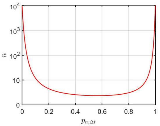
Given $p_{n,\mathsf{\Delta }t}\in (0,1)$, we compute the value of n needed such that $\left|S_T^{\left(n\right)}-S_T\right|\le {10}^{-4}$. In the limit $(n\uparrow \infty ,\mathsf{\Delta }t\downarrow 0)$, the importance of $p_{n,\mathsf{\Delta }t}$ vanishes since the trader taking a short position in $\mathcal{C}$ is allowed to trade continuously in time (which, indeed, is a fiction in real trading).

We argue that an option trader should use the information incorporated in the estimates of the probability $p_{n,\mathsf{\Delta }t}$. To emphasize this point, we provide estimates for $p_{n,\mathsf{\Delta }t}$ based on 25.5 years of the SPDR S&P 500 ETF (SPY)29 historical price data. We use a window of one year to construct a moving window strategy to estimate

$${\widehat{p}}_{n,\mathsf{\Delta }t}=\frac{\mathrm{number} \mathrm{of} \mathrm{days} \mathrm{with} \mathrm{non}\text{-}\mathrm{negative} \log \text{-}\mathrm{return} \mathrm{in} \mathrm{the} \mathrm{current} \mathrm{window}}{\mathrm{total} \mathrm{number} \mathrm{of} \mathrm{days} \mathrm{in} \mathrm{the} \mathrm{current} \mathrm{window}}.$$

The estimates for ${\widehat{p}}_{n,\mathsf{\Delta }t}$ are shown in Figure 2.

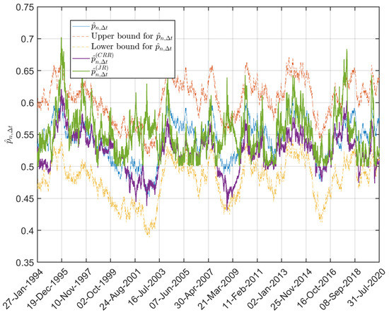
Figure 2. Values of ${\widehat{p}}_{n\mathsf{\Delta }t}$ of the SPY daily log-returns computed from a one-year moving window over the time period 27 January 1994 to 31 July 2020. Additionally displayed are values for ${\widehat{p}}_{n\mathsf{\Delta }t}^{\left(\mathrm{CRR}\right)}$ and ${\widehat{p}}_{n\mathsf{\Delta }t}^{\left(\mathrm{JR}\right)}$ computed as described in Section 3.1.

We split the time series ${\widehat{p}}_{n,\mathsf{\Delta }t}$ into non-overlapping intervals (weeks, months, and years) and apply the two-sided sign test on each interval with $H_0:p_{n,\mathsf{\Delta }t}=1/2$. Figure 3 shows the results for the hypothesis test in terms of box-whisker plots of the p-values.

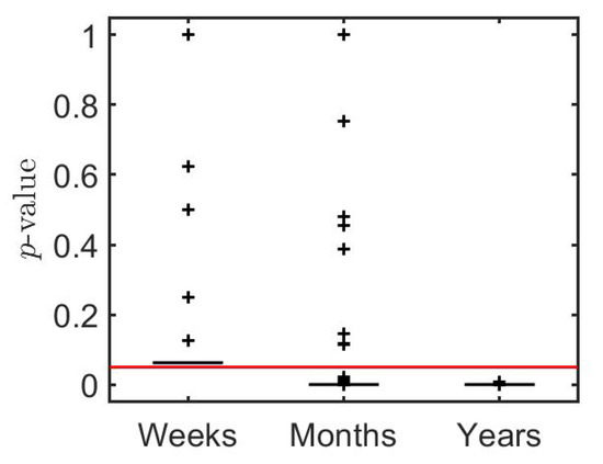
Figure 3. Box-whisker plots of the p-values for two-sided sign tests on the values of ${\widehat{p}}_{n\mathsf{\Delta }t}$ of the SPY daily log-returns shown in Figure 2. The solid red line indicates the 0.05 significance level.

The plots: indicate there is insufficient evidence to reject $H_0$ at the $0.05$ significance level for weekly intervals; imply rejection of $H_0$ in most monthly intervals; and imply rejection of $H_0$ in all yearly intervals.

3. General Binomial Option Pricing

Following the framework of the CRR-binomial pricing model, our next goal was to use the general binomial tree (5) to derive the discrete price dynamics $f_{t_{n,k}}^{\left(n\right)},k=0,\dots ,k_{n-1}$ of an ECC having terminal payoff $f_T^{\left(n\right)}=G\left(S_{t_{n,k_n}}\right)$. For $k=0,1,\dots ,k_n-1$, consider the replicating risk-neutral portfolio $P_{t_{n,k}}^{\left(n\right)}=D_{t_{n,k}}^{\left(n\right)}{S}_{t_{n,k}}^{\left(n\right)}-f_{t_{n,k}}^{\left(n\right)}$, $P_{t_{n,k+1}}^{\left(n\right)}=D_{t_{n,k}}^{\left(n\right)}{S}_{t_{n,k+1}}^{\left(n\right)}-f_{t_{n,k+1}}^{\left(n\right)}$, with $D_{t_n,k}^{\left(n\right)}$ being the “delta” position, and $S_{t_{n,k+1}}^{\left(n\right)}$ determined by the pricing tree (5). From the hedge position,

$$D_{t_{n,k}}^{\left(n\right)}{S}_{t_{n,k+1}}^{(n,u)}-f_{t_{n,k+1}}^{(n,u)}=D_{t_{n,k}}^{\left(n\right)}{S}_{t_{n,k+1}}^{(n,d)}-f_{t_{n,k+1}}^{(n,d)},$$

it follows

$$\begin{array}{cc}\hfill D_{t_{n,k}}^{\left(n\right)}& =\frac{f_{t_{n,k+1}}^{(n,u)}-f_{t_{n,k+1}}^{(n,d)}}{S_{t_{n,k}}^{\left(n\right)}{e}^{\mu \mathsf{\Delta }{t}_{n,k+1}}\left\{e^{M_1}-e^{M_2}\right\}},\hfill \end{array}$$

(6)

where

$$\begin{array}{cc}\hfill M_1& =-\frac{1-p_{n,k+1}}{p_{n,k+1}}\frac{{\sigma }^2}{2}\mathsf{\Delta }{t}_{n,k+1}+\sigma \sqrt{\frac{1-p_{n,k+1}}{p_{n,k+1}}}\sqrt{\mathsf{\Delta }{t}_{n,k+1}},\hfill \\ \hfill M_2& =-\frac{p_{n,k+1}}{1-p_{n,k+1}}\frac{{\sigma }^2}{2}\mathsf{\Delta }{t}_{n,k+1}-\sigma \sqrt{\frac{p_{n,k+1}}{1-p_{n,k+1}}}\sqrt{\mathsf{\Delta }{t}_{n,k+1}}.\hfill \end{array}$$

As $f_{t_{n,k}}^{\left(n\right)}=D_{t_{n,k}}^{\left(n\right)}{S}_{t_{n,k}}^{\left(n\right)}-e^{-r\mathsf{\Delta }{t}_{n,k+1}}{P}_{t_{n,k+1}}^{(n,u)}$, we have

$$f_{t_{n,k}}^{\left(n\right)}=e^{-r\mathsf{\Delta }{t}_{n,k+1}}\left\{q_{n,k+1}{f}_{t_{n,k+1}}^{(n,u)}+(1-q_{n,k+1})f_{t_{n,k+1}}^{(n,d)}\right\},$$

where the risk-neutral upturn probability $q_{n,k+1}$ for the time period $[t_{n,k},t_{n,k+1})$ is given by

$$q_{n,k+1}=\frac{e^{(r-\mu )\mathsf{\Delta }{t}_{n,k+1}}-e^{M_2}}{e^{M_1}-e^{M_2}},$$

(7)

with $M_1$ and $M_2$ defined in (6). Assuming all terms of order $o\left(\mathsf{\Delta }{t}_{n,k}\right)$ are negligible in (7), we have

$$q_{n,k}=p_{n,k}-\theta \sqrt{p_{n,k}(1-p_{n,k})\mathsf{\Delta }{t}_{n,k}},k=1,\dots ,k_n,n\in \mathcal{N},$$

(8)

where $\theta =(\mu -r)/\sigma$ is the market price of risk.

Furthermore, the delta-position $D_{t_{n,k}}^{\left(n\right)}$ in (6) becomes

$$D_{t_{n,k}}^{\left(n\right)}=\frac{\left(f_{t_{n,k+1}}^{(n,u)}-f_{t_{n,k+1}}^{(n,d)}\right)\sqrt{p_{n,k+1}(1-p_{n,k+1})}}{S_{t_{n,k}}^{\left(n\right)}{e}^{\mu \mathsf{\Delta }{t}_{n,k+1}}\sigma \sqrt{\mathsf{\Delta }{t}_{n,k+1}}}.$$

Thus, as $p_{n,k+1}\uparrow 1$ or $p_{n,k+1}\downarrow 0$, the delta-position $D_{t_{n,k}}^{\left(n\right)}\to 0$, since if $p_{n,k+1}=0$ or $p_{n,k+1}=1,k=0,1,\dots ,k_n$, the ECC becomes a fixed-income security and no hedging is needed.

We now consider the risk-neutral dynamics,

$$S_{t_{n,k}}^{(n,q)}=\left\{\begin{array}{cc}{S}_{t_{n,k}}^{(n,q,u)}\hfill & =S_{t_{n,k-1}}^{(n,q)}exp\left\{\left(\mu -\frac{1-p_{n,k}}{p_{n,k}}\frac{{\sigma }^2}{2}\right)\mathsf{\Delta }{t}_{n,k}+\sigma \sqrt{\frac{1-p_{n,k}}{p_{n,k}}}\sqrt{\mathsf{\Delta }{t}_{n,k}}\right\},\mathrm{if}{\varsigma }_{n,k}^{\left(q\right)}=1,\hfill \\ S_{t_{n,k}}^{(n,q,d)}\hfill & =S_{t_{n,k-1}}^{(n,q)}exp\left\{\left(\mu -\frac{p_{n,k}}{1-p_{n,k}}\frac{{\sigma }^2}{2}\right)\mathsf{\Delta }{t}_{n,k}-\sigma \sqrt{\frac{p_{n,k}}{1-p_{n,k}}}\sqrt{\mathsf{\Delta }{t}_{n,k}}\right\},\mathrm{if}{\varsigma }_{n,k}^{\left(q\right)}=-1,\hfill \end{array}\right.$$

(9)

where ${\varsigma }_{n,k}^{\left(q\right)},k=1,\dots ,k_n$ are independent binary random variables with $\mathbb{P}({\varsigma }_{n,k}^{\left(q\right)}=1)=1-\mathbb{P}({\varsigma }_{n,k}^{\left(q\right)}=-1)=q_{n,k}\in (0,1),k=1,\dots ,k_n,n\in \mathcal{N}$. The discrete risk-neutral log-return process, $R_{t_{n,k}}^{(n,q)}=ln\left(S_{t_{n,k}}^{(n,q)}/S_{t_{n,k-1}}^{(n,q)}\right)$, has mean $\mathbb{E}\left(R_{t_{n,k}}^{(n,q)}\right)=\left(r-\frac{{\sigma }^2}{2}\right)\mathsf{\Delta }{t}_{n,k}$ and variance $\mathrm{Var}\left(R_{t_{n,k}}^{(n,q)}\right)={\sigma }^2\mathsf{\Delta }{t}_{n,k}$. Set

$$\begin{array}{cc}\hfill {\mathbb{S}}_{[0,T]}^{(n,q)}& =\left\{S_t^{(n,q)}=S_{t_{n,k}}^{(n,q)},t\in [t_{n,k},t_{n,k+1}),k=0,\dots ,k_{n-1},S_{t_n,0}^{(n,q)}=S_0,S_T^{(n,q)}=S_{t_{n,k_n}}^{(n,q)}\right\},\hfill \\ \hfill {\mathbb{S}}_{[0,T]}^{\left(q\right)}& =\left\{S_t^{\left(q\right)}=S_{0}exp\left\{\left(r-\frac{{\sigma }^2}{2}\right)t+\sigma B_t^{\left(q\right)}\right\},t\in [0,T]\right\},\hfill \end{array}$$

(10)

where ${\mathbb{B}}_{[0,T]}^{\left(q\right)}={\left\{B_t^{\left(q\right)}\right\}}_{0\le t\le T}$ is a standard BM. Then, using the same arguments as in Section 2.2, we have that ${\mathbb{S}}_{[0,T]}^{(n,q)}$ converges weakly to ${\mathbb{S}}_{[0,T]}^{\left(q\right)}$ in $(\mathcal{D}[0,T],d^{\left(0\right)})$.

3.1. Comparison with CRR and JR Models

If $p_{n,k}=p_{n,\mathsf{\Delta }t}=p^{\left(0\right)}+p^{\left(1\right)}\sqrt{\mathsf{\Delta }t}+p^{\left(2\right)}\mathsf{\Delta }t,k=1,\dots ,k_n,\mathsf{\Delta }t=T/n$, then from (8)

$$q_{n,k}=q_{n,\mathsf{\Delta }t}≔p^{\left(0\right)}+\left(p^{\left(1\right)}-\theta \sqrt{p^{\left(0\right)}(1-p^{\left(0\right)})}\right)\sqrt{\mathsf{\Delta }t}+\left(p^{\left(2\right)}-\frac{\theta }{2}\frac{p^{\left(1\right)}(1-2p^{\left(0\right)})}{\sqrt{p^{\left(0\right)}(1-p^{\left(0\right)})}}\right)\mathsf{\Delta }t.$$

In the CRR model, the risk-neutral probability for non-negative stock log-returns in period $k\mathsf{\Delta }t,\mathsf{\Delta }t=T/n,n\uparrow \infty$ is given by $q_{n,k}^{\left(\mathrm{CRR}\right)}=q_{n,\mathsf{\Delta }t}^{\left(\mathrm{CRR}\right)}=\frac{exp\left(r\mathsf{\Delta }t\right)-exp(-\sigma \sqrt{\mathsf{\Delta }t})}{exp\left(\sigma \sqrt{\mathsf{\Delta }t}\right)-exp(-\sigma \sqrt{\mathsf{\Delta }t})}=1/2+\frac{r-{\sigma }^2/2}{2\sigma }\sqrt{\mathsf{\Delta }t}$. According to (8), the corresponding natural probability $p_{n,k}^{\left(\mathrm{CRR}\right)}=p_{n,\mathsf{\Delta }t}^{\left(\mathrm{CRR}\right)}$ is given by $p_{n,\mathsf{\Delta }t}^{\left(\mathrm{CRR}\right)}=1/2+\frac{\mu -{\sigma }^2/2}{2\sigma }\sqrt{\mathsf{\Delta }t}$. In the JR model, $q_{n,k}^{\left(\mathrm{JR}\right)}=q^{\left(\mathrm{JR}\right)}=1/2$. If $\mathsf{\Delta }t=T/n$ then, as $n\uparrow \infty$, the corresponding probability for stock-upturn in the JR model is given by $p_{n,k}^{\left(\mathrm{JR}\right)}=p_{n,\mathsf{\Delta }t}^{\left(\mathrm{JR}\right)}=1/2+\left|\theta \right|\sqrt{\mathsf{\Delta }t}$. Figure 2 also plots estimates ${\widehat{p}}_{\mathsf{\Delta }t}^{\left(\mathrm{CRR}\right)},{\widehat{p}}_{\mathsf{\Delta }t}^{\left(\mathrm{JR}\right)}$ of the values for $p_{\mathsf{\Delta }t}^{\left(\mathrm{CRR}\right)}$ and $p_{\mathsf{\Delta }t}^{\left(\mathrm{JR}\right)}$ using the SPY data of Section 2.3 and compares them with the estimated values ${\widehat{p}}_{\mathsf{\Delta }t}$ for $p_{\mathsf{\Delta }t}$. Again, we apply a two-sided sign test with the following hypotheses:

$$\left\{\begin{array}{c}{H}_0^{\left(\mathrm{CRR}\right)}:p_{\mathsf{\Delta }t}=p_{\mathsf{\Delta }t}^{\left(\mathrm{CRR}\right)};\hfill \\ H_a^{\left(\mathrm{CRR}\right)}:p_{\mathsf{\Delta }t}\ne p_{\mathsf{\Delta }t}^{\left(\mathrm{CRR}\right)};\hfill \end{array}\right.\left\{\begin{array}{c}{H}_0^{\left(\mathrm{JR}\right)}:p_{\mathsf{\Delta }t}=p_{\mathsf{\Delta }t}^{\left(\mathrm{JR}\right)};\hfill \\ H_a^{\left(\mathrm{JR}\right)}:p_{\mathsf{\Delta }t}\ne p_{\mathsf{\Delta }t}^{\left(\mathrm{JR}\right)};\hfill \end{array}\right.$$

to the sample estimates generated on non-overlapping intervals (weeks, months, and years). The results from the two-sided sign tests are shown as box-whisker plots in Figure 4a,b. They produce conclusions somewhat similar to those of Figure 3. In the case of weekly intervals in both figures, there is no sufficient evidence to reject $H_0^{\left(\mathrm{CRR}\right)}$ ($H_0^{\left(\mathrm{JR}\right)}$) at the 0.05 significance level, whereas for monthly and year intervals, the results indicate rejection of $H_0^{\left(\mathrm{CRR}\right)}$ ($H_0^{\left(\mathrm{JR}\right)}$) in most intervals.

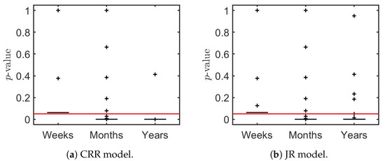
Figure 4. Box-whisker plots of the p-values for two-sided sign tests on the values of ${\widehat{p}}_{n\mathsf{\Delta }t}^{\left(\mathrm{CRR}\right)}$ and ${\widehat{p}}_{n\mathsf{\Delta }t}^{\left(\mathrm{JR}\right)}$ shown in Figure 2. The solid red line indicates the 0.05 significance level.

3.2. Rate of Loss of $\mu$ as Hedging Rate Increases

In continuous-time option pricing, the mean log-return parameter $\mu$ and the information about the market direction embedded in $p_{n,k}$ are lost due to the artificial assumption that hedging can be done continuously in time with no transaction costs. We can estimate the rate of loss of $\mu$ from (10) by computing the dependence of the number of necessary hedging instances, $n=T/\mathsf{\Delta }t$ on $\mu$ while requiring that $\parallel S_T^{(n,q)}-S_T^{\left(q\right)}\parallel \le {10}^{-4}$. The results over the range $\mu \in [0,50]$ are shown in Figure 5. From he figure we deduce that $n\uparrow \infty$ as $\mu \uparrow \infty$. From these results we conclude that, in continuous option pricing, $\mu$ disappears as a model parameter due to the (practically inconceivable) use of continuous time hedging.

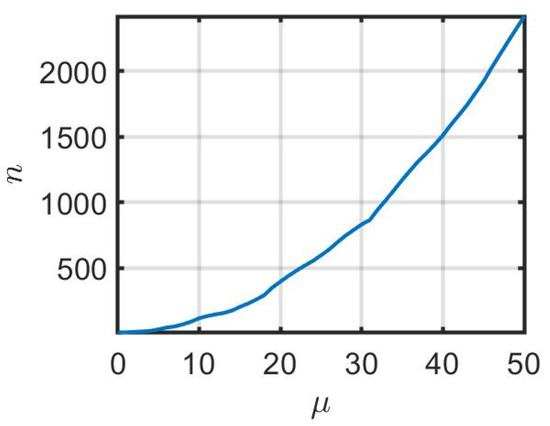
Figure 5. Convergence rate, measured as $n=T/\mathsf{\Delta }t$, of $S_T^{(n,q)}$ to $S_T^{\left(q\right)}$ in (10) as a function of $\mu$ over the range $\mu \in (0,50)$. In this simulation, $r=0$, $p_{n,\mathsf{\Delta }t}=0.5$, $\sigma =1$, $T=1$ and convergence was considered achieved when $|(S_T^{(n,q)}-S_T^{\left(q\right)})/S_0|\le {10}^{-6}$.

3.3. Estimation of the Implied Risk-Neutral Probability $q_{n,\mathsf{\Delta }t}$

We estimate the risk-neutral probability $q_{n,\mathsf{\Delta }t}$ in (8) based on XSP.30 Denote the call option prices by $C_t^{\left(\mathrm{XSP}\right)}(K,T-t)$, where K is the strike price, and T is the terminal time. We assume that hedging occurs daily, that is, $\mathsf{\Delta }{t}_{n,k}=k\mathsf{\Delta }t,k=1,\dots ,n,n=T/\mathsf{\Delta }t$. Then, (8) becomes $q_{n,\mathsf{\Delta }t}=p_{n,\mathsf{\Delta }t}-\theta \sqrt{p_{n,\mathsf{\Delta }t}(1-p_{n,\mathsf{\Delta }t})\mathsf{\Delta }t}$ and through terms of $O\left(\mathsf{\Delta }t\right)$,

$$p_{n,\mathsf{\Delta }t}=q_{n,\mathsf{\Delta }t}+\left|\theta \right|\sqrt{q_{n,\mathsf{\Delta }t}\left(1-q_{n,\mathsf{\Delta }t}\right)\mathsf{\Delta }t}+\left(\frac{1}{2}-q_{n,\mathsf{\Delta }t}\right){\theta }^2\mathsf{\Delta }t.$$

(11)

The XSP call options data were collected on 31 July 2020 with initial capital $S_0^{\left(\mathrm{SPY}\right)}=326.52$ and annual risk-free rate31 $r=0.55\%$. We estimated $\mu$ and $\sigma$ using the mean and standard derivation of the log-return of SPY for the one-year window from 2 August 2019 to 31 July 2020. This window produced the estimates $\widehat{\mu }=6.20\times {10}^{-4}$ and $\widehat{\sigma }=0.02$. Following the framework established in Section 3 and (11), we can view the theoretical value of the call options $C_t^{\left(\mathrm{XSP};\mathrm{theoretical}\right)}(S_0^{\left(\mathrm{SPY}\right)},K,T-t,q_{n,\mathsf{\Delta }t})$ as a function of $q_{n,\mathsf{\Delta }t}$. For different strike price K and time t, we can estimate $q_{n,\mathsf{\Delta }t}$ via

$${\widehat{q}}_{n,\mathsf{\Delta }t}=\arg \min \left\{{\left(\frac{C_t^{\left(\mathrm{XSP};\mathrm{theoretical}\right)}(S_0^{\left(\mathrm{SPY}\right)},K,T-t,q_{n,\mathsf{\Delta }t})-C_t^{\left(\mathrm{XSP}\right)}(K,T-t)}{C_t^{\left(\mathrm{XSP}\right)}(K,T-t)}\right)}^2\right\}.$$

Figure 6 presents the implied ${\widehat{q}}_{n,\mathsf{\Delta }t}$, the corresponding implied ${\widehat{p}}_{n,\mathsf{\Delta }t}$, and ${\widehat{q}}_{n,\mathsf{\Delta }t}-{\widehat{p}}_{n,\mathsf{\Delta }t}$ surfaces. All figures are graphed against the standard measures of moneyness and time to maturity (in days). From Figure 6a, ${\widehat{q}}_{n,\mathsf{\Delta }t}$ ranges from 0.5 to 0.62. Given these values of ${\widehat{q}}_{n,\mathsf{\Delta }t}$ and values of r, $\sigma$ and $\mu$, Equation (11) shows that ${\widehat{p}}_{n,\mathsf{\Delta }t}$ = ${\widehat{q}}_{n,\mathsf{\Delta }t}+O\left({10}^{-3}\right)$.32

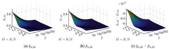
Figure 6. Implied surfaces for ${\widehat{q}}_{n,\mathsf{\Delta }t}$, ${\widehat{p}}_{n,\mathsf{\Delta }t}$, and ${\widehat{q}}_{n,\mathsf{\Delta }t}-{\widehat{p}}_{n,\mathsf{\Delta }t}$ plotted as functions of time to maturity T and moneyness $M=K/S$.

As a result, Figure 6b shows that ${\widehat{p}}_{n,\mathsf{\Delta }t}$ varies from 0.51 to 0.63. For a fixed T, ${\widehat{p}}_{n,\mathsf{\Delta }t}$ has a higher value as $M\in (1,1.5)$ compared to when $M\in (0.5,1)$. For any value of M, ${\widehat{p}}_{n,\mathsf{\Delta }t}$ decreases as time to maturity increases. Recall that $p_{n,\mathsf{\Delta }t}$ is the natural probability for an upward movement (or non-negative log-return) of the stock price over the time period $\mathsf{\Delta }t$, and $q_{n,\mathsf{\Delta }t}$ is the corresponding risk-neutral probability for an upward movement of the stock price. Thus the implied surface indicates that, on the trading day 31 July 2020, the option traders of SPY were optimistic (bullish) for the coming six-month period.

4. Cherny–Shiryaev–Yor Invariance Principle and Path-Dependent Stock Log-Return Dynamics

In this section, we formulate a new binomial path-dependent pricing model where the stock price dynamics depends on the log-return dynamics of a market index. Our approach is based on an extension of the Donsker–Prokhorov invariance principle due to Cherny et al. (2003). We start with the formulation of the Cherny–Shiryaev–Yor invariance principle (CSYIP). Let ${\xi }_k,k\in \mathcal{N}$ be a sequence of independent and identically distributed (i.i.d.) random variables with mean 0 and variance 1. Set ${\xi }_0^{\left(n\right)}=0,{\xi }_k^{\left(n\right)}=n^{-\frac{1}{2}}{\xi }_k$, and $X_{k/n}^{\left(n\right)}={\sum }_{i=1}^k{\xi }_i^{\left(n\right)},k\in \mathcal{N},n\in \mathcal{N}$. Let ${\mathbb{B}}_t^{\left(n\right)},t\ge 0$ be the random process with piecewise linear trajectories having vertices $(k/n,{\mathbb{B}}_{k/n}^{\left(n\right)})$, where ${\mathbb{B}}_{k/n}^{\left(n\right)}=X_{k/n}^{\left(n\right)},k\in \mathcal{N},n\in \mathcal{N}$. Following Cherny et al. (2003), call a function $h:R\to R$ a CSY piecewise continuous function if there exists a collection of disjoint intervals $J_n,n\in \mathcal{N}$33 such that:

(i)

${\cup }_{n=1}^{\infty }{J}_n=R$;

(ii)

for every compact interval J, there exists $n\in \mathcal{N}$ such that ${\cup }_{k=1}^n{J}_k\supseteq J$;

(iii)

on each $J_n,n\in \mathcal{N}$, the function $h:J_n\to R$ is continuous, and has finite limits at those endpoints of $J_n$ which do not belong to $J_n$.

Let $Y_{k/n}^{\left(n\right)}={\sum }_{i=1}^{k}h\left(X_{(i-1)/n}^{\left(n\right)}\right){\xi }_i^{\left(n\right)},k\in \mathcal{N},n\in \mathcal{N}$. For every fixed $n\in \mathcal{N}$, define ${\mathbb{C}}_t^{\left(n\right)},t\ge 0$ to be the random process with CSY piecewise linear trajectories having vertexes $(k/n,{\mathbb{C}}_{k/n}^{\left(n\right)})$, where ${\mathbb{C}}_{k/n}^{\left(n\right)}=Y_{k/n}^{\left(n\right)},k\in \mathcal{N},n\in \mathcal{N}$.

(CSYIP) If $h:R\to R$ is a CSY piecewise continuous function, then, as $n\uparrow \infty$, the bivariate process $({\mathbb{B}}_t^{\left(n\right)},{\mathbb{C}}_t^{\left(n\right)}),t\ge 0$ converges in law34 to $(B_t,C_t),t\ge 0$, where $B_t$ is a standard BM and $C_t={\int }_0^{t}h\left(B_s\right)d{B}_s$.

In the CRR- and JR-binomial models, as well as in the general binomial model (5), the stock log-returns are assumed independent. Based on CSYIP, we introduce a binomial tree model in which the log-returns are dependent on a sequence of random signs representing the past history of the movement of a market index influencing the stock’s dynamics. Let $S_{t_{n,k}}^{(n,M)},t_{n,k}=k\mathsf{\Delta }t,k=1,\dots ,n,n\mathsf{\Delta }t=T,n\in N$, with $S_{t_{n,0}}^{(n,M)}=S_0^{(n,M)}=S_0^{\left(M\right)}>0$, be a market index value for the period $[t_{n,k},t_{n,k+1})$. Let $R_{t_{n,k}}^{(n,M,hist)}=ln\left(S_{t_{n,k}}^{(n,M,hist)}/S_{t_{n,k-1}}^{(n,M,hist)}\right)$ be the historical market index log-return (index-return for brevity) in the $k^{th}$ period, and ${\varsigma }_{n,k}^{\left(M\right)},k=1,\dots ,n$, be the binary sequence of the index’s value directions: ${\varsigma }_{n,k}^{\left(M\right)}=1$, if $R_{t_{n,k}}^{(n,M,hist)}\ge 0$, and ${\varsigma }_{n,k}^{\left(M\right)}=-1$, if $R_{t_{n,k}}^{(n,M,hist)}<0$. We assume that ${\varsigma }_{n,k}^{\left(M\right)},k=1,\dots ,n$, are independent random signs, with $\mathbb{P}({\varsigma }_{n,k}^{\left(M\right)}=1)=1-\mathbb{P}({\varsigma }_{n,k}^{\left(M\right)}=-1)=p_{n,\mathsf{\Delta }t}^{\left(M\right)}=p_0^{\left(M\right)}+p_1^{\left(M\right)}\sqrt{\mathsf{\Delta }t}+p_2^{\left(M\right)}\mathsf{\Delta }t$. We further assume $p_0^{\left(M\right)}\in (0,1),p_1^{\left(M\right)}\in R,p_2^{\left(M\right)}\in R,\mathsf{\Delta }t=\frac{T}{n}\downarrow 0$ so that $p_{n,\mathsf{\Delta }t}^{\left(M\right)}\in (0,1)$. We model the market index price dynamics (index-dynamics for brevity) as

$$S_{t_{n,k}}^{(n,M)}=S_{t_{n,k-1}}^{(n,M)}exp\left\{R_{t_{n,k}}^{(n,M)}\right\},$$

(12)

where

$$R_{t_{n,k}}^{(n,M)}=\left\{\begin{array}{c}\left({\mu }^{\left(M\right)}-\frac{1-p_{n,\mathsf{\Delta }t}^{\left(M\right)}}{p_{n,\mathsf{\Delta }t}^{\left(M\right)}}\frac{{{\sigma }^{\left(M\right)}}^2}{2}\right)\mathsf{\Delta }t+{\sigma }^{\left(M\right)}\sqrt{\frac{1-p_{n,\mathsf{\Delta }t}^{\left(M\right)}}{p_{n,\mathsf{\Delta }t}^{\left(M\right)}}}\sqrt{\mathsf{\Delta }t},\mathrm{if}{\varsigma }_{n,k}^{\left(M\right)}=1,\hfill \\ \left({\mu }^{\left(M\right)}-\frac{p_{n,\mathsf{\Delta }t}^{\left(M\right)}}{1-p_{n,\mathsf{\Delta }t}^{\left(M\right)}}\frac{{{\sigma }^{\left(M\right)}}^2}{2}\right)\mathsf{\Delta }t-{\sigma }^{\left(M\right)}\sqrt{\frac{p_{n,\mathsf{\Delta }t}^{\left(M\right)}}{1-p_{n,\mathsf{\Delta }t}^{\left(M\right)}}}\sqrt{\mathsf{\Delta }t},\mathrm{if}{\varsigma }_{n,k}^{\left(M\right)}=-1,\hfill \end{array}\right.$$

(13)

with ${\mu }^{\left(M\right)}>r>0$, and ${\sigma }^{\left(M\right)}>0$ determined from the historical log-return data. As shown in Section 2.1, if

$$\begin{array}{cc}\hfill {\mathbb{S}}_{[0,T]}^{(n,M)}& =\left\{S_t^{(n,M)}=S_{t_{n,k}}^{(n,M)},t\in [t_{n,k},t_{n,k+1}),k=0,\cdots ,n-1;S_{t_n,0}^{(n,M)}=S_0,S_T^{(n,M)}=S_{t_{n,n}}^{(n,M)}\right\},\hfill \\ \hfill {\mathbb{S}}_{[0,T]}^{\left(M\right)}& =\left\{S_t^{\left(M\right)}=S_{0}exp\left\{\left({\mu }^{\left(M\right)}-\frac{{{\sigma }^{\left(M\right)}}^2}{2}\right)t+{\sigma }^{\left(M\right)}{B}_t\right\},t\in [0,T]\right\},\hfill \end{array}$$

then the discrete market index price dynamics ${\mathbb{S}}_{[0,T]}^{(n,M)}$ converge weakly to ${\mathbb{S}}_{[0,T]}^{\left(M\right)}$ in $(\mathcal{D}[0,T],d^{\left(0\right)})$.

We apply CSYIP by setting

$$\begin{array}{c}\left(a\right)Z_{n,k}^{\left(M\right)}=\frac{1}{{\sigma }^{\left(M\right)}\sqrt{\mathsf{\Delta }t}}\left(R_{t_{n,k}}^{(n,M)}-\left({\mu }^{\left(M\right)}-\frac{{{\sigma }^{\left(M\right)}}^2}{2}\right)\mathsf{\Delta }t\right),\hfill \\ \left(b\right){\xi }_{n,k}^{\left(M\right)}=\sqrt{\frac{1-{\mathsf{𝕡}}_{n,\mathsf{\Delta }t}^{\left(M\right)}}{{\mathsf{𝕡}}_{n,\mathsf{\Delta }t}^{\left(M\right)}}}{I}_{\left\{Z_{n,k}^{\left(M\right)}\ge 0\right\}}-\sqrt{\frac{{\mathsf{𝕡}}_{n,\mathsf{\Delta }t}^{\left(M\right)}}{1-{\mathsf{𝕡}}_{n,\mathsf{\Delta }t}^{\left(M\right)}}}{I}_{\left\{Z_{n,k}^{\left(M\right)}<0\right\}},\hfill \\ \left(c\right)X_{k/n}^{\left(n\right)}=\sum _{i=1}^k\sqrt{\mathsf{\Delta }t}{\xi }_{n,i}^{\left(M\right)},\hfill \\ \left(d\right)Y_{k/n}^{(n,h)}=\sum _{i=1}^k\sqrt{\mathsf{\Delta }t}{\xi }_{n,i}^{\left(M\right)}h\left(X_{(i-1)/n}^{\left(n\right)}\right),\hfill \end{array}$$

(14)

where ${\mathsf{𝕡}}_{n,\mathsf{\Delta }t}^{\left(M\right)}=\mathbb{P}\left(Z_{n,k}^{\left(M\right)}\ge 0\right)\in (0,1)$ is the probability for an upturn in the index’s centralized log-return $Z_{n,k}^{\left(M\right)}$. The random signs ${\xi }_{n,k}^{\left(M\right)},k=1,\dots ,n$, are independent with $\mathbb{E}\left({\xi }_{n,k}^{\left(M\right)}\right)=0$ and $\mathrm{Var}\left({\xi }_{n,k}^{\left(M\right)}\right)=1$. Consider the following processes in the Skorokhod space $\mathcal{D}[0,T]$,

$$\begin{array}{cc}\hfill {\mathbb{B}}_{[0,T]}^{\left(n\right)}& =\left\{B_t^{\left(n\right)}=X_{k/n}^{\left(n\right)},t\in [t_{n,k},t_{n,k+1}),k=0,\dots ,n-1;B_0^{\left(n\right)}=X_0^{\left(n\right)}=0,B_T^{\left(n\right)}=X_1^{\left(n\right)}\right\},\hfill \\ \hfill {\mathbb{C}}_{[0,T]}^{(n,h)}& =\left\{C_t^{(n,h)}=Y_{k/n}^{(n,h)},t\in [t_{n,k},t_{n,k+1}),k=0,\dots ,n-1;C_0^{(n,h)}=Y_0^{(n,h)}=0,C_T^{(n,h)}=Y_1^{(n,h)}\right\}.\hfill \end{array}$$

(15)

According to CSYIP, as $n\uparrow \infty$, the bivariate process $\left({\mathbb{B}}_{[0,T]}^{\left(n\right)},{\mathbb{C}}_{[0,T]}^{(n,h)}\right)$ converges weakly in $\mathcal{D}[0,T]\times \mathcal{D}[0,T]$ to $\left({\mathbb{B}}_{[0,T]},{\mathbb{C}}_{[0,T]}^{\left(h\right)}\right)$, where ${\mathbb{B}}_{[0,T]}={\left\{B_t\right\}}_{0\le t\le T}$ is a BM on $[0,T]$, and ${\mathbb{C}}_{[0,T]}^{\left(h\right)}={\left\{C_t^{\left(h\right)}={\int }_0^{t}h\left(B_s\right)d{B}_s\right\}}_{0\le t\le T}$.

Next, we define the stock price discrete dynamics as a functional of ${\mathbb{B}}_{[0,T]}^{\left(n\right)}$ and ${\mathbb{C}}_{[0,T]}^{(n,h)}$. Let

$$\begin{array}{cc}\hfill {\mathbb{S}}_{[0,T]}^{(n,h,S)}=& \left\{S_t^{(n,h,S)}=S_0^{\left(S\right)}exp\left[\nu t_{n,k}+\sigma B_t^{\left(n\right)}+\gamma C_t^{(n,h)}\right],t\in [t_{n,k},t_{n,k+1}),k=0,\dots ,n-1,\right.\hfill \\ \hfill & \left.S_T^{(n,h,S)}=S_0^{\left(S\right)}exp\left[\nu T+\sigma B_T^{\left(n\right)}+\gamma C_T^{(n,h)}\right]\right\},\hfill \end{array}$$

(16)

where $\nu >r>0,\sigma >0,\gamma \ge 0$ are parameters determining the dynamics of the stock price as a function of the index dynamics. Then, as $n\uparrow \infty$, ${\mathbb{S}}_{[0,T]}^{(n,h,S)}$ converges weakly to ${\mathbb{S}}_{[0,T]}^{(h,S)}=\left\{S_0^{\left(S\right)}exp\left\{\nu t+\sigma B_t+\gamma C_t^{\left(h\right)}\right\},t\in [0,T]\right\}$ in $\mathcal{D}[0,T]$. The stock discrete log-return dynamics is given by

$$R_{t_{n,k}}^{(n,h,S)}=ln\left(\frac{S_{t_{n,k}}^{(n,h,S)}}{S_{t_{n,k-1}}^{(n,h,S)}}\right)=\nu \mathsf{\Delta }t+\sigma \sqrt{\mathsf{\Delta }t}{\xi }_{n,k}^{\left(M\right)}+\gamma \sqrt{\mathsf{\Delta }t}{\xi }_{n,k}^{\left(M\right)}h\left(\sum _{i=1}^{k-1}\sqrt{\mathsf{\Delta }t}{\xi }_{n,i}^{\left(M\right)}\right).$$

(17)

Thus, when $\gamma \ne 0$, the stock log-return $R_{t_{n,k}}^{(n,h,S)}$ depends on the entire path $\left\{{\xi }_{n,i}^{\left(M\right)},i=1,\dots ,k\right\}$ of market return intensity. As a result, the $R_{t_{n,k}}^{(n,h,S)},k=1,\dots ,n$, are dependent log-returns when $\gamma \ne 0$.

4.1. An Extension of the Cherny–Shiryaev–Yor Invariance Principle

In this section, we extend CSYIP to obtain a more flexible model for the stock price. We extend (14a–d) by adding the term,

$$\begin{array}{c}\hfill \left(e\right)V_{k/n}^{(n,g)}=\sum _{i=1}^k\sqrt{\mathsf{\Delta }t}{\xi }_{n,i}^{\left(M\right)}g\left(\sum _{j=1}^{i-1}\left(\sum _{l=1}^{j-1}\sqrt{\mathsf{\Delta }t}{\xi }_{n,l}^{\left(M\right)}\right)\mathsf{\Delta }t\right),\end{array}$$

where $g:R\to R$ is a CSY piecewise continuous function. Together with the processes ${\mathbb{B}}_{[0,T]}^{\left(n\right)}$ and ${\mathbb{C}}_{[0,T]}^{(n,h)}$ in (15), we consider the additional $\mathcal{D}[0,T]$-process,

$${\mathbb{G}}_{[0,T]}^{(n,g)}=\left\{G_t^{(n,h)}=V_{k/n}^{(n,g)},t\in [t_{n,k},t_{n,k+1}),k=0,\dots ,n-1,G_0^{(n,h)}=V_0^{(n,g)}=0,G_T^{(n,g)}=V_1^{(n,g)}\right\},$$

and define the stock price discrete dynamics as a functional of ${\mathbb{B}}_{[0,T]}^{\left(n\right)}$, ${\mathbb{C}}_{[0,T]}^{(n,h)}$, and ${\mathbb{G}}_{[0,T]}^{(n,g)}$ by

$$\begin{array}{cc}\hfill {\mathbb{S}}_{[0,T]}^{(n,h,g,S)}=& \left\{S_t^{(n,h,g,S)}=S_0^{\left(S\right)}exp\left[\nu t_{n,k}+\sigma B_t^{\left(n\right)}+\gamma C_t^{(n,h)}+\delta G_t^{(n,g)}\right],t\in [t_{n,k},t_{n,k+1}),k=0,\dots ,n-1,\right.\hfill \\ \hfill & \left.S_T^{(n,h,g,S)}=S_0^{\left(S\right)}exp\left[\nu T+\sigma B_T^{\left(n\right)}+\gamma C_T^{(n,h)}+\delta G_T^{(n,g)}\right]\right\},\hfill \end{array}$$

(18)

where $\nu >r>0,\sigma >0,\gamma >0,\delta >0$. As for the CSYIP discrete process, ${\mathbb{S}}_{[0,T]}^{(n,h,g,S)}$ converges weakly to

$${\mathbb{S}}_{[0,T]}^{(h,g,S)}=\left\{S_t^{(h,g,S)}=S_0^{\left(S\right)}exp\left[\nu t+\sigma B_t+\gamma C_t^{\left(h\right)}+\delta G_t^{\left(g\right)}\right],t\in [0,T],S_0^{\left(S\right)}>0,\right\}$$

(19)

in $\mathcal{D}[0,T]$ as $n\uparrow \infty$, where: $B_t$ is a standard BM; $C_t^{\left(h\right)}={\int }_0^{t}h\left(B_{\nu }\right)d{B}_{\nu }$; and $G_t^{\left(g\right)}={\int }_0^{t}g\left({\int }_0^{\nu }{B}_{u}du\right)d{B}_{\nu }$. The stock discrete log-return dynamics is given by

$$\begin{array}{cc}\hfill & R_{t_{n,k}}^{(n,h,g,S)}=ln\left(\frac{S_{t_{n,k}}^{(n,h,g,S)}}{S_{t_{n,k-1}}^{(n,h,g,S)}}\right)\hfill \\ \hfill & =\nu \mathsf{\Delta }t+\sigma \sqrt{\mathsf{\Delta }t}{\xi }_{n,k}^{\left(M\right)}+\gamma \sqrt{\mathsf{\Delta }t}{\xi }_{n,k}^{\left(M\right)}h\left(\sum _{i=1}^{k-1}\sqrt{\mathsf{\Delta }t}{\xi }_{n,i}^{\left(M\right)}\right)+\delta \sqrt{\mathsf{\Delta }t}{\xi }_{n,k}^{\left(M\right)}g\left(\sum _{j=1}^{k-1}\left(\sum _{l=1}^{j-1}\sqrt{\mathsf{\Delta }t}{\xi }_{n,l}^{\left(M\right)}\right)\mathsf{\Delta }t\right).\hfill \end{array}$$

(20)

The new term captures additional long-range dependence in $R_{t_{n,k}}^{(n,h,g,S)}$. While the argument of the $h\left(\right)$ function on the right-hand side of (20) weights past terms of ${\xi }_{n,i}^{\left(M\right)}$ equally in the summation, the double summation in the argument of the $g\left(\right)$ function has the effect of linearly weighting the ${\xi }_{n,i}^{\left(M\right)}$, with the weight decreasing toward present time.35 Of course the (potentially non-linear) CSY piecewise continuous function $g\left(\right)$ plays a role in mutating the long-range dependence introduced by its argument. The Appendix A to this paper provides a deeper numerical investigation of the behavior of the terms in (20) using MSFT for the stock and S&P500 for the market index. In particular it is shown that the choice of Gaussian functional forms for $h\left(\right)$ and $g\left(\right)$ act as band-pass filters on the informational content of their arguments. Using a series of non-overlapping one-year time periods, the predictive ability of the model (20) is examined. Finally the behavior of the discrete form (20) is compared to its continuum analog (19).

4.2. An Example

As an example of stock return dynamics depending on market intensity path, we consider the daily price process $S_{k\mathsf{\Delta }t}^{(n,\mathrm{MSFT})}$ of MSFT as a function of the trajectory of the S&P index dynamics. MSFT and S&P 500 price data for the period 1 July 2019 through 30 June 2020 were obtained from Yahoo Finance. From this period we estimated the mean ${\mu }^{\left(\mathrm{S}\&\mathrm{P}\right)}$ and standard deviation ${\sigma }^{\left(\mathrm{S}\&\mathrm{P}\right)}$ of the log-returns process $R_{t_{n,k}}^{(n,\mathrm{S}\&\mathrm{P})}$ of the S&P 500 index. The sample estimates are denoted ${\widehat{\mu }}^{\left(\mathrm{S}\&\mathrm{P}\right)}$ and ${\widehat{\sigma }}^{\left(\mathrm{S}\&\mathrm{P}\right)}$. We apply CSYIP by assuming that the S&P 500 index-return daily intensity follows (14) with

$$Z_{t_{n,k}}^{(n,\mathrm{S}\&\mathrm{P})}=\frac{1}{{\widehat{\sigma }}^{\left(\mathrm{S}\&\mathrm{P}\right)}\sqrt{\mathsf{\Delta }t}}\left(R_{t_{n,k}}^{(n,\mathrm{S}\&\mathrm{P})}-\left({\widehat{\mu }}^{\left(\mathrm{S}\&\mathrm{P}\right)}-\frac{{\widehat{\sigma }}^{{\left(\mathrm{S}\&\mathrm{P}\right)}^2}}{2}\right)\mathsf{\Delta }t\right).$$

(21)

and

$${\xi }_{t_{n,k}}^{\left(\mathrm{S}\&\mathrm{P}\right)}=\sqrt{\frac{1-{\mathsf{𝕡}}_{n,\mathsf{\Delta }t}^{\left(\mathrm{S}\&\mathrm{P}\right)}}{{\mathsf{𝕡}}_{n,\mathsf{\Delta }t}^{\left(\mathrm{S}\&\mathrm{P}\right)}}}{I}_{\left\{Z_{t_{n,k}}^{(n,\mathrm{S}\&\mathrm{P})}\ge 0\right\}}-\sqrt{\frac{{\mathsf{𝕡}}_{n,\mathsf{\Delta }t}^{\left(\mathrm{S}\&\mathrm{P}\right)}}{1-{\mathsf{𝕡}}_{n,\mathsf{\Delta }t}^{\left(\mathrm{S}\&\mathrm{P}\right)}}}{I}_{\left\{Z_{t_{n,k}}^{(n,\mathrm{S}\&\mathrm{P})}<0\right\}},$$

(22)

where ${\mathsf{𝕡}}_{n,\mathsf{\Delta }t}^{\left(\mathrm{S}\&\mathrm{P}\right)}=\mathbb{P}\left(Z_{t_{n,k}}^{(n,\mathrm{S}\&\mathrm{P})}\ge 0\right)\in (0,1)$. For simplicity, we choose $h\left(x\right)={\left({\sigma }_h\sqrt{2\pi }\right)}^{-1}exp[-x^2/\left(2{\sigma }_h^2\right)]$, $g\left(x\right)={\left({\sigma }_g\sqrt{2\pi }\right)}^{-1}exp[-x^2/\left(2{\sigma }_g^2\right)]$, $x\in R$ in (20).36 With “$\left(M\right)=\left(\mathrm{S}\&\mathrm{P}\right)$” in (20), the historical log-return time series, $R_{t_{n,k}}^{(n,\mathrm{MSFT},\mathrm{hist})}$, for MSFT can be fit by the model

$$\begin{array}{cc}\hfill R_{t_{n,k}}^{(n,\mathrm{MSFT},\mathrm{hist})}& =\nu \mathsf{\Delta }t+\sigma \sqrt{\mathsf{\Delta }t}{\xi }_{n,k}^{\left(\mathrm{S}\&\mathrm{P}\right)}+\gamma \sqrt{\mathsf{\Delta }t}{\xi }_{n,k}^{\left(\mathrm{S}\&\mathrm{P}\right)}h\left(\sum _{i=1}^{k-1}\sqrt{\mathsf{\Delta }t}{\xi }_{n,i}^{\left(\mathrm{S}\&\mathrm{P}\right)}\right)\hfill \\ \hfill & +\delta \sqrt{\mathsf{\Delta }t}{\xi }_{n,k}^{\left(\mathrm{S}\&\mathrm{P}\right)}g\left(\sum _{j=1}^{k-1}\left(\sum _{l=1}^{j-1}\sqrt{\mathsf{\Delta }t}{\xi }_{n,l}^{\left(\mathrm{S}\&\mathrm{P}\right)}\right)\mathsf{\Delta }t\right)+{ϵ}_{t_{n,k}}^{(n,\mathrm{MSFT})},\hfill \end{array}$$

(23)

where ${ϵ}_{t_{n,k}}^{(n,\mathrm{MSFT})}$ are the error terms in the above regression model denoting the MSFT stock-specific risk. To solve for the model parameters, we construct the minimization problem

$$\underset{\nu >r>0,\sigma >0,\gamma >0,\delta >0}{min}{\parallel {ϵ}_{t_{n,k}}^{(n,\mathrm{MSFT})}\parallel }_2^2.$$

(24)

The minimization problem (24) can be regarded as a conditional least squares optimizing problem, which provides consistent estimates under suitable assumptions (Pešta and Okhrin 2014). We note that the solution space of this constrained, non-linear minimization problem37 is very unstable; small perturbations away from a parameter solution set, when used as new parameter guesses to initialize the minimization problem, can produce a radically different solution having the same minimizing RMSE. Table 1 (rows S&P${}^a$ and S&P${}^b$) present the parameter estimates for two solutions which, to three significant digits, have the same values for RMSE. Of the two solutions, S&P${}^a$ is more realistic since $\sigma =0$ for S&P${}^b$.

Table 1. Parameter estimates obtained from the minimization problem (24).

Factor	$\mathit{\nu }$	$\mathit{\sigma }$	$\mathit{\gamma }$	${\mathit{\sigma }}_{\mathit{h}}$	$\mathit{\delta }$	${\mathit{\sigma }}_{\mathit{g}}$	RMSE
S&P${}^a$	0.0016	0.0020	0.29	8.8	0.089	$1.8\times {10}^3$	0.0214
S&P${}^b$	0.0016	$1.1\times {10}^{-10}$	0.37	9.9	0.44	0.052	0.0214
S&P Hist	$2.2\times {10}^{-14}$	0.014	0.0014	0.13	1.09	0.10	0.0214
S&P with ARMA(1,1)-GJR GARCH(1,1) innovations modeled by:
ghyp	0.0013	$2.2\times {10}^{-14}$	0.0078	0.073	0.35	0.072	0.0254
stud t	0.0017	$4.4\times {10}^{-14}$	0.011	0.22	1.1	0.10	0.0252
norm	0.0018	$2.2\times {10}^{-14}$	0.0038	0.077	1.1	0.10	0.0253
J${}^a$	0.0019	0.0065	0.083	73	0.11	$7.6\times {10}^4$	0.0244
J${}^b$	0.0020	0.0062	0.0000	0.0027	0.84	$1.1\times {10}^2$	0.0244
FF3${}^a$	0.0019	0.0049	0.012	$9.7\times {10}^3$	0.0008	$1.0\times {10}^4$	0.0249
FF3${}^b$	0.0018	0.0044	0.0068	0.59	1.09	$3.1\times {10}^5$	0.0249

Equation (23) models MSFT returns in terms of systematic risk from the S&P 500 index based on the up- and down-turns of the centralized log-return (21). We consider the case where the systematic risk is determined directly by the up- and down-turns of $R_{t_{n,k}}^{(n,\mathrm{S}\&\mathrm{P})}$, i.e.,

$${\xi }_{n,k}^{\left(\mathrm{S}\&\mathrm{P}\right)}=\left\{\begin{array}{c}1\mathrm{if}{R}_{t_{n,k}}^{(n,\mathrm{S}\&\mathrm{P})}\ge 0,\hfill \\ -1\mathrm{if}{R}_{t_{n,k}}^{(n,\mathrm{S}\&\mathrm{P})}<0.\hfill \end{array}\right.$$

This has the effect of setting ${\mathsf{𝕡}}_{n,\mathsf{\Delta }t}^{\left(\mathrm{S}\&\mathrm{P}\right)}=p_{n,\mathsf{\Delta }t}^{\left(\mathrm{S}\&\mathrm{P}\right)}$. One solution of this subsequent minimization (24) are shown in Table 1 (row S&P Hist). In terms of RMSE, this approach appears equivalent to the first.

We have also explored a third option for the minimization (23).38 The centralized return $Z_{n,k}^{\left(M\right)}$ defined in (14) implicitly treats $R_{t_{n,k}}^{(n,M)}$ as if they were i.i.d. normally distributed (Gaussian noise). Knowing this is not true, we performed an “ARMA(1,1)-GJR GARCH(1,1) with assumed innovation distribution” fit

$$\begin{array}{c}\hfill \begin{array}{cc}\hfill R_{k,\mathsf{\Delta }t}^{(n,\mathrm{S}\&\mathrm{P})}& =\mu +{\varphi }_1(R_{k-1,\mathsf{\Delta }t}^{(n,\mathrm{S}\&\mathrm{P})}-\mu )+a_k+{\theta }_1{a}_{k-1},\hfill \\ \hfill a_k& ={\sigma }_k{ϵ}_k,\hfill \\ \hfill {\sigma }_k^2& ={\alpha }_0+({\alpha }_1+{\gamma }_1{I}_{k-1})a_{k-1}^2+{\beta }_1{\sigma }_{k-1}^2,\hfill \end{array}\end{array}$$

(25)

to the log-returns $R_{k,\mathsf{\Delta }t}^{(n,\mathrm{S}\&\mathrm{P})}$ of the market index. For the innovation distribution we assumed either standardized-Gaussian, -Student’s t, or -generalized hyperbolic. Denote the resultant time series of residuals obtained from this ARMA-GJR GARCH fit as ${ϵ}_{n,k}^{AG,D}$ where D identifies the distribution used in the fit. By filtering out the ARMA-GARCH factors, the series ${ϵ}_{n,k}^{AG,D}$ should be “noise” (though perhaps not Gaussian). Following (14), the time series ${ϵ}_{n,k}^{AG,D}$ replaces $R_{k,\mathsf{\Delta }t}^{(n,\mathrm{S}\&\mathrm{P})}$ in (21) and the subsequent steps leading to the construction of the minimization problem (23).

The results of the ARMA-GJR GARCH fit using the Student’s t and generalized hyperbolic distributions are given in Table 2. Parameter solutions for the minimization problem (23) using the residuals ${ϵ}_{n,k}^{AG,norm}$, ${ϵ}_{n,k}^{AG,studt}$, and ${ϵ}_{n,k}^{AG,ghyp}$ are shown in the correspondingly labeled rows in Table 1. Based upon RMSE values, this option provides less predictive power than direct use of $R_{k,\mathsf{\Delta }t}^{(n,\mathrm{S}\&\mathrm{P})}$.

Table 2. ARMA(1,1)-GJR GARCH(1,1) with standardized Student’s t and generalized hyperbolic innovation fits to the residuals ${ϵ}_{t_{n,k}}^{(n,\mathrm{MSFT})}$ of (23).

	Student’s t				Generalized Hyperbolic
Parameter	Estimate	SE	t-Value	p-Value	Estimate	SE	t-Value	p-Value
$\mu$	$4.0\times {10}^{-5}$	$6\times {10}^{-4}$	0.067	0.94	$4.0\times {10}^{-5}$	$6.5\times {10}^{-4}$	0.06	0.95
${\varphi }_1$	$0.32$	0.37	0.87	0.38	0.30	0.40	0.77	0.44
${\theta }_1$	−0.45	0.35	−1.3	0.19	−0.44	0.37	−1.2	0.24
${\alpha }_0$	$1.2\times {10}^{-5}$	$3.7\times {10}^{-5}$	0.32	0.75	$1.2\times {10}^{-5}$	$9.0\times {10}^{-6}$	1.46	0.14
${\alpha }_1$	0.24	0.35	0.68	0.50	0.24	0.13	1.82	0.07
${\beta }_1$	0.727	0.024	29	0	0.724	0.05	14	0
${\gamma }_1$	−0.10	0.14	−0.67	0.51	−0.11	0.16	−0.68	0.50
shape (${\nu }^a,{\zeta }^b$)	13	6.3	2.05	0.04	2.5	58	0.04	0.97
skew (${\rho }^b$)					−0.31	7.5	−0.04	0.97
${\lambda }^b$					−5.8	42	−0.14	0.89
Robust standard errors
parameter	estimate	SE	t-value	p-value	estimate	SE	t-value	p-value
$\mu$	$4.0\times {10}^{-5}$	0.0024	0.017	0.99	$4.0\times {10}^{-5}$	$7.4\times {10}^{-4}$	0.054	0.96
${\varphi }_1$	$0.32$	0.79	0.41	0.68	0.30	0.51	0.60	0.55
${\theta }_1$	−0.45	0.64	−0.71	0.48	−0.44	0.44	−1.0	0.32
${\alpha }_0$	$1.2\times {10}^{-5}$	$3.6\times {10}^{-4}$	0.034	0.97	$1.2\times {10}^{-5}$	$2.6\times {10}^{-5}$	0.48	0.63
${\alpha }_1$	0.24	3.4	0.070	0.94	0.24	0.38	0.64	0.52
${\beta }_1$	0.727	0.52	1.4	0.16	0.724	0.089	8.1	0
${\gamma }_1$	−0.10	0.18	−0.54	0.59	−0.11	0.31	−0.34	0.73
shape (${\nu }^a,{\zeta }^b$)	13	110	0.12	0.91	2.5	343	0.007	0.99
skew (${\rho }^b$)					−0.31	43	−0.007	0.99
${\lambda }^b$					−5.8	229	−0.026	0.98

${}^a$ The shape factor $\nu$ for the standardized Student’s t distribution is the degrees of freedom. ${}^b$ The rugarch package in R uses the $\zeta ,\rho ,\lambda$ parameterization for the standardized generalized hyperbolic distribution. See Introduction to the rugarch package. (Version 1.4-3) A. Ghalanos, 15 July 2020.

In addition to using the log-return process of the S&P 500 index as a model for the MSFT log-return dynamics, we also considered models based upon time series of “implied alphas”. The first is based upon Jensen’s alpha39 while the second is the implied alpha determined from the Fama-French three-factor (FF3) model40.

The Jensen alpha time-series was computed as

$${\alpha }_{k\mathsf{\Delta }t}^{\left(\mathrm{J}\right)}=R_{k\mathsf{\Delta }t}^{\left(\mathrm{MSFT}\right)}-R_{f,k\mathsf{\Delta }t}-{\beta }^{\left(\mathrm{J}\right)}\left[R_{k\mathsf{\Delta }t}^{\left(\mathrm{S}\&\mathrm{P}\right)}-R_{f,k\mathsf{\Delta }t}\right]$$

(26)

where $k\mathsf{\Delta }t$ ran over the daily trading days from 1 July 2019 through 30 June 2020. Daily return values for the risk-free rate $R_{f,k\mathsf{\Delta }t}$ were computed from the 10-year Treasury rates and returns from the S&P 500 were used to represent the market. Single values for ${\beta }^{\left(\mathrm{J}\right)}$ and ${\alpha }^{\left(\mathrm{J}\right)}$ were computed using a linear regression for (26) over the entire data set. A time series of daily values of ${\alpha }_{k\mathsf{\Delta }t}^{\left(\mathrm{J}\right)}$ were then computed using (26). The values of this implied Jensen’s alpha time-series replaced the S&P 500 index values in the above analysis (22) through (24).

A time series of implied values of ${\alpha }_{k\mathsf{\Delta }t}^{\left(\mathrm{FF}3\right)}$ were computed analogously. Daily values for $R_m$, $R_f$, $R_{\mathrm{SMB}}$, and $R_{\mathrm{HML}}$ were obtained from the U.S. Research Returns Data page of Professor French’s web site41. Again, single values for the FF3 constants ${\beta }^{\left(M\right)}$, ${\beta }^{\left(\mathrm{SMB}\right)}$ and ${\beta }^{\left(\mathrm{HML}\right)}$ were obtained from linear regression using the entire data set. Using these, daily values for ${\alpha }_{k\mathsf{\Delta }t}^{\left(\mathrm{FF}3\right)}$ were computed.

Parameter values obtained from the minimization problem (24) for each implied alpha time series are also displayed in Table 1 (rows J and FF3, respectively). Based on RMSE values, the Jensen and FF3 alpha models are poorer predictors than $R_{k,\mathsf{\Delta }t}^{(n,\mathrm{S}\&\mathrm{P})}$ for the dynamics of the returns of MSFT within the discrete pricing model (20), but are better than option 3.

To test for clustering of the volatility and/or heavy tails, we fit the residuals ${ϵ}_{t_{n,k}}^{(n,\mathrm{MSFT})}$ in (23) to an ARMA(1,1)-GARCH(1,1) model (Equation (25) with ${\gamma }_1=0$) with Student’s t innovations. Using the residuals ${ϵ}_{t_{n,k}}^{(n,\mathrm{MSFT})}$ obtained from the fit in row S&P${}^a$ in Table 1, Table 3 reports the results for the fitted parameters as well as the p-values obtained. The p-values indicate that the fit to the GARCH component of the model (25) is significant at the 5% level, while the fits to the Student’s t-distribution (degrees of freedom) and, particularly, the ARMA component are much less so.

Table 3. Parameter estimates for fitting the sample residuals ${ϵ}_{t_{n,k}}^{(n,MSFT)}$ to the ARMA-GARCH form of (25).

	Estimate	Standard Error	t-Statistic	p-Value
$\mu$	0.00	0.00	0.52	0.6
${\varphi }_1$	0.33	0.44	0.74	0.45
${\theta }_1$	−0.45	0.42	−1.08	0.28
${\alpha }_0$	0.00	0.00	2.08	0.04
${\alpha }_1$	0.71	0.07	10.85	0.00
${\beta }_1$	0.25	0.08	3.36	0.00
${\nu }^a$	13.7	12.75	1.07	0.28

${}^a\nu$ is degrees of freedom of Student’s t distribution.

Figure 7 compares the fitted Student’s t-distribution for 13 degrees of freedom with the empirical values of ${ϵ}_k$ computed from the ARMA-GARCH form of (25) using the parameters in Table 3. The comparison shows that the tails of the distribution of sample residuals, ${ϵ}_{t_{n,k}}^{\ast }$, are not exponentially bounded. In addition, the sample residual distribution is not symmetric, but is skewed to the right. Overall, the model (25) does not capture the empirical phenomena displayed by the MSFT stock over this time period.

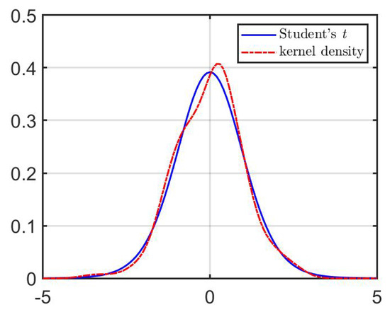
Figure 7. Comparison of the standardized Student’s t-distribution with $\nu =13$ compared to the empirical distribution of ${ϵ}_k$ computed from (25).

5. Option Pricing When the Underlying Stock Log-Returns Are Path-Dependent

In this section, we use the path-dependent dynamics of the underlying stock price in continuous-time as given by (19), and in discrete-time as given by (18), to derive the corresponding risk-neutral dynamics and to value the ECC $\mathcal{C}$. We first consider the continuous-time stock price dynamics $S_t^{(h,g,S)},t\in [0,T]$ on $\left(\mathsf{\Omega },\mathbb{F}={\left\{{\mathcal{F}}_t=\sigma \left(B_u\right)\right\}}_{u\le t},\mathbb{P}\right)$ in (19). Using Itô’s formula, we have

$$\begin{array}{cc}\hfill d{S}_t^{(h,g,S)}& =N_1{S}_t^{(h,g,S)}dt+N_2{S}_t^{(h,g,S)}d{B}_t,\hfill \end{array}$$

(27)

where

$$\begin{array}{cc}\hfill N_1& =\nu +\frac{1}{2}{\sigma }^2+\frac{1}{2}{\gamma }^2{h\left(B_t\right)}^2+\frac{1}{2}{\delta }^2{\left(g\left({\int }_0^t{B}_{u}du\right)\right)}^2+\sigma \gamma h\left(B_t\right)+\sigma \delta g\left({\int }_0^t{B}_{u}du\right)\hfill \\ \hfill & +\gamma \delta h\left(B_t\right)g\left({\int }_0^t{B}_{u}du\right),\hfill \\ \hfill N_2& =\sigma +\gamma h\left(B_t\right)+\delta g\left({\int }_0^t{B}_{u}du\right).\hfill \end{array}$$

From (27), the risk-neutral stock price dynamics are defined by

$$\begin{array}{cc}\hfill d{S}_t^{(h,g,S)}& =r{S}_t^{(h,g,S)}dt+N_2{S}_t^{(h,g,S)}d{B}_t^{\left(\mathbb{Q}\right)},t\in [0,T],\hfill \end{array}$$

(28)

where $S_0^{(h,g,S)}=S_0^{\left(S\right)}$. In (28), $B_t^{\mathbb{Q}}=B_t+{\int }_0^t{\theta }_{s}ds$ is a BM on $\mathbb{Q}$ and the market price of risk ${\theta }_t,t\in [0,T]$, is given by ${\theta }_t=(N_1-r)/N_2$. As a result that ${\theta }_t$ is uniquely determined for $t\ge 0$, $(\mathcal{S},\mathcal{B})$ is an arbitrage-free and complete market. Let $f_t=f(S_t,t),t\in [0,T]$, denote the price dynamics of the ECC $\mathcal{C}$ with terminal time $T>0$ and final payoff $f_T=G\left(S_T\right)$. Then, $f_0=e^{-rT}{\mathbb{E}}^{\left(\mathbb{Q}\right)}G\left(S_T\right)$ under the usual regularity conditions (Duffie 2001).

Consider the discrete filtration ${\mathbb{F}}^{\left(d\right)}=\left\{{\mathcal{F}}_0=\{⌀,\mathsf{\Omega }\},{\mathcal{F}}_k=\sigma ({\xi }_{n,1}^{\left(M\right)},\dots ,{\xi }_{n,k}^{\left(M\right)}),k=1,\dots ,n,n\in \mathcal{N}\right\}$, where ${\xi }_{n,k}^{\left(M\right)}$ is given by (14). Let

$${\eta }_{k,\mathsf{\Delta }t}^{\left(M\right)}=\sigma +\gamma h\left(\sum _{i=1}^k\sqrt{\mathsf{\Delta }t}{\xi }_{n,i+1}^{\left(M\right)}\right)+\delta g\left(\sum _{j=1}^k\left(\sum _{l=1}^{j-1}\sqrt{\mathsf{\Delta }t}{\xi }_{n,l}^{\left(M\right)}\right)\mathsf{\Delta }t\right)>0,k=1,\dots ,n,$$

(29)

with ${\eta }_{0,\mathsf{\Delta }t}^{\left(M\right)}=\sigma ,\nu >r>0,\sigma >0,\gamma >0,\delta >0$, and $h\left(x\right)\ge 0,g\left(x\right)\ge 0,x\in R$ are uniformly bounded piecewise continuous functions. According to (20), the stock binomial tree dynamics conditioned on ${\mathcal{F}}_k$ is given by

$$\begin{array}{cc}\hfill S_{(k+1)\mathsf{\Delta }t}^{(n,h,g,S)}& =S_{k\mathsf{\Delta }t}^{(n,h,g,S)}exp\left\{\nu \mathsf{\Delta }t+{\eta }_{k,\mathsf{\Delta }t}^{\left(M\right)}\sqrt{\mathsf{\Delta }t}{\xi }_{n,k+1}^{\left(M\right)}\right\},S_0^{(h,g,S)}=S_0,k=0,1,\dots ,n-1.\hfill \end{array}$$

(30)

Note that ${\eta }_{k,\mathsf{\Delta }t}^{\left(M\right)}$ represents the time-varying stock volatility at $k\mathsf{\Delta }t$ as a function of index intensities ${\xi }_{n,i}^{\left(M\right)},i=1,\dots ,n$. From (14), conditionally on ${\mathcal{F}}_k,k=0,\dots ,n-1$, we have

$$S_{(k+1)\mathsf{\Delta }t}^{(n,h,g,S)}=\left\{\begin{array}{cc}{S}_{(k+1)\mathsf{\Delta }t}^{(n,h,g,S,u)}\hfill & =S_{k\mathsf{\Delta }t}^{(n,h,g,S)}exp\left\{\nu \mathsf{\Delta }t+{\eta }_{k,\mathsf{\Delta }t}^{\left(M\right)}\sqrt{\mathsf{\Delta }t}\sqrt{\frac{1-{\mathsf{𝕡}}_{n,\mathsf{\Delta }t}^{\left(M\right)}}{{\mathsf{𝕡}}_{n,\mathsf{\Delta }t}^{\left(M\right)}}}\right\},\mathrm{w}.\mathrm{p}.{\mathsf{𝕡}}_{n,\mathsf{\Delta }t}^{\left(M\right)},\hfill \\ S_{(k+1)\mathsf{\Delta }t}^{(n,h,g,S,d)}\hfill & =S_{k\mathsf{\Delta }t}^{(n,h,g,S)}exp\left\{\nu \mathsf{\Delta }t-{\eta }_{k,\mathsf{\Delta }t}^{\left(M\right)}\sqrt{\mathsf{\Delta }t}\sqrt{\frac{{\mathsf{𝕡}}_{n,\mathsf{\Delta }t}^{\left(M\right)}}{1-{\mathsf{𝕡}}_{n,\mathsf{\Delta }t}^{\left(M\right)}}}\right\},\mathrm{w}.\mathrm{p}.1-{\mathsf{𝕡}}_{n,\mathsf{\Delta }t}^{\left(M\right)}.\hfill \end{array}\right.$$

(31)

Then, similarly to the derivation of (8), we obtain the conditional risk-neutral probabilities

$${\mathsf{𝕢}}_{k,\mathsf{\Delta }t}^{\left(S\right)}={\mathsf{𝕡}}_{n,\mathsf{\Delta }t}^{\left(M\right)}-{\theta }_{k,\mathsf{\Delta }t}^{\left(S\right)}\sqrt{{\mathsf{𝕡}}_{n,\mathsf{\Delta }t}^{\left(M\right)}(1-{\mathsf{𝕡}}_{n,\mathsf{\Delta }t}^{\left(M\right)})\mathsf{\Delta }t},{\theta }_{k,\mathsf{\Delta }t}^{\left(S\right)}=\frac{\nu -r}{{\eta }_{k,\mathsf{\Delta }t}^{\left(M\right)}},k=0,\dots ,n-1,n\in \mathcal{N}.$$

(32)

Conditionally on ${\mathcal{F}}_k$, the stock risk-neutral dynamics is given by $S_0^{(n,\mathsf{𝕢})}=S_0$, and for $k=0,\dots ,n-1$,

$$S_{(k+1)\mathsf{\Delta }t}^{(n,\mathsf{𝕢})}=\left\{\begin{array}{cc}{S}_{(k+1)\mathsf{\Delta }t}^{(n,\mathsf{𝕢},u)}\hfill & =S_{k\mathsf{\Delta }t}^{(n,\mathsf{𝕢})}exp\left\{\nu \mathsf{\Delta }t+{\eta }_{k,\mathsf{\Delta }t}^{\left(M\right)}\sqrt{\mathsf{\Delta }t}\sqrt{\frac{1-{\mathsf{𝕡}}_{n,\mathsf{\Delta }t}^{\left(M\right)}}{{\mathsf{𝕡}}_{n,\mathsf{\Delta }t}^{\left(M\right)}}}\right\},\mathrm{w}.\mathrm{p}.{\mathsf{𝕢}}_{k,\mathsf{\Delta }t}^{\left(S\right)},\hfill \\ S_{(k+1)\mathsf{\Delta }t}^{(n,\mathsf{𝕢},d)}\hfill & =S_{k\mathsf{\Delta }t}^{(n,\mathsf{𝕢})}exp\left\{\nu \mathsf{\Delta }t-{\eta }_{k,\mathsf{\Delta }t}^{\left(M\right)}\sqrt{\mathsf{\Delta }t}\sqrt{\frac{{\mathsf{𝕡}}_{n,\mathsf{\Delta }t}^{\left(M\right)}}{1-{\mathsf{𝕡}}_{n,\mathsf{\Delta }t}^{\left(M\right)}}}\right\},\mathrm{w}.\mathrm{p}.1-{\mathsf{𝕢}}_{k,\mathsf{\Delta }t}^{\left(S\right)}.\hfill \end{array}\right.$$

(33)

In (32), the market price of risk ${\theta }_{k,\mathsf{\Delta }t}^{\left(S\right)}$ is time dependent, leading to a heavy-tailed distribution for the log-returns $R_{(k+1)\mathsf{\Delta }t}^{(n,\mathsf{𝕢})}=ln\left(S_{(k+1)\mathsf{\Delta }t}^{(n,\mathsf{𝕢})}/S_{k\mathsf{\Delta }t}^{(n,\mathsf{𝕢})}\right)$ in (33), which can produce a more realistic pricing model for the EEC $\mathcal{C}$. The risk-neutral price $f_{k\mathsf{\Delta }t}^{\left(n\right)}=f\left(S_{k\mathsf{\Delta }t}^{(n,\mathsf{𝕢})},k\mathsf{\Delta }t\right)$ of $\mathcal{C}$ is given by

$$f_{k\mathsf{\Delta }t}^{\left(n\right)}=e^{-r\mathsf{\Delta }t}\left\{{\mathsf{𝕢}}_{k,\mathsf{\Delta }t}^{\left(S\right)}{f}_{k\mathsf{\Delta }t}^{(n,u)}+(1-{\mathsf{𝕢}}_{k,\mathsf{\Delta }t}^{\left(S\right)})f_{k\mathsf{\Delta }t}^{(n,d)}\right\},$$

where $f_{(k+1)\mathsf{\Delta }t}^{(n,u)}=f\left(S_{(k+1)\mathsf{\Delta }t}^{(n,\mathsf{𝕢},u)},(k+1)\mathsf{\Delta }t\right)$, $f_{(k+1)\mathsf{\Delta }t}^{(n,d)}=f\left(S_{(k+1)\mathsf{\Delta }t}^{(n,\mathsf{𝕢},d)},(k+1)\mathsf{\Delta }t\right)$, $k=0,\dots ,n-1$, and $f_{n\mathsf{\Delta }t}^{\left(n\right)}=f_T^{\left(n\right)}=G\left(S_T\right)$.

An Example

We apply CSYIP to generate an artificial binomial tree to obtain call option prices using the daily closing prices and the corresponding log-return process of MSFT combined with the parameter estimations of row S&P${}^a$ in Table 1. Using the daily intensity dynamics ${\xi }_{t_{n,k}}^{\left(\mathrm{S}\&\mathrm{P}\right)}$ in (22), we have

$${\eta }_{k,\mathsf{\Delta }t}^{\left(\mathrm{S}\&\mathrm{P}\right)}=\widehat{\sigma }+\widehat{\gamma }h\left(\sum _{i=1}^k\sqrt{\mathsf{\Delta }t}{\xi }_{n,i+1}^{\left(\mathrm{S}\&\mathrm{P}\right)}\right)+\widehat{\delta }g\left(\sum _{j=1}^k\left(\sum _{l=1}^{j-1}\sqrt{\mathsf{\Delta }t}{\xi }_{n,l}^{\left(\mathrm{S}\&\mathrm{P}\right)}\right)\mathsf{\Delta }t\right),$$

(34)

where $\widehat{\sigma },\widehat{\gamma }$, and $\widehat{\delta }$ are given in row S&P${}^a$ of Table 1. Following the framework developed in (27) through (33) based on the MSFT price data and the 10-year Treasury rate42, we obtain the call option price $C_t^{\left(\mathrm{MSFT};\mathrm{CSY}\right)}(S_0^{\left(\mathrm{MSFT}\right)},K,T,\widehat{\nu },\widehat{\sigma },\widehat{\gamma },\widehat{\delta })$. Using the Black–Scholes–Merton formula43, we calculate the corresponding CSY implied volatility ${\sigma }^{(\mathrm{CSY}-\mathrm{vol})}$. We compare it to the implied volatility based on the call options data for MSFT from the Chicago Board Option Exchange (CBOE), which we denote as ${\sigma }^{(\mathrm{CBOE}-\mathrm{vol})}$, by defining the relative volatility deviation,

$${\mathrm{DEV}}^{(\mathrm{CSY}-\mathrm{CBOE})}=\frac{{\sigma }^{(\mathrm{CSY}-\mathrm{vol})}-{\sigma }^{(\mathrm{CBOE}-\mathrm{vol})}}{{\sigma }^{(\mathrm{CSY}-\mathrm{vol})}}.$$

${\mathrm{DEV}}^{(\mathrm{CSY}-\mathrm{CBOE})}$ can be used to identify mispricing of various option contracts based on the deviation of the existing market implied volatility surface from the theoretical ${\sigma }^{(\mathrm{CSY}-\mathrm{vol})}$. Figure 8 shows values of DEV${}^{(\mathrm{CSY}-\mathrm{CBOE})}$ ranging from −0.68 to 2.01, with an increasing trend as T increases.

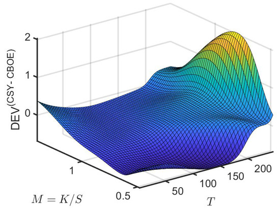
Figure 8. Relative volatility deviation against time to maturity T and moneyness $M=K/S$.

6. Option Pricing for Markets with Informed Traders

We extend the results of Section 5 to option pricing for markets with informed traders. Suppose that at $(k-1)\mathsf{\Delta }t,k=1,\dots ,n,n\mathsf{\Delta }t=T$, a trader (denoted by ℵ) observed the market index closing values $S_{j\mathsf{\Delta }t}^{(n,M)},j=0,1,\dots ,k-1$, with the corresponding values of $Z_{t_{n,k}}^{(n,M)}$ given by (14a). Consequently, ℵ knows the probability ${\mathsf{𝕡}}_{\mathsf{\Delta }t}^{(\aleph ,M)}\in (1/2,1)$ for the sign of $Z_{k\mathsf{\Delta }t}^{(n,M)}.$44 ℵ assumes that the continuous time dynamics of the stock price $S_t^{(h,g,S)}$ is given by (19). The risk-free asset dynamics are given by

$${\beta }_t={\beta }_0{e}^{{\int }_0^t{r}_{u}du},{\beta }_0>0,t\in [0,T],$$

(35)

where $r_t,t\in [0,T]$ is the instantaneous risk-free rate.45

The discrete filtration ${\mathbb{F}}^{\left(d\right)}$ defined in Section 5 defines the discrete dynamics of the market index. From (31), define the binomial tree conditioned on ${\mathcal{F}}_k$ as

$$S_{(k+1)\mathsf{\Delta }t}^{(n,h,g)}=\left\{\begin{array}{cc}{S}_{(k+1)\mathsf{\Delta }t}^{(n,h,g,u)}\hfill & =S_{k\mathsf{\Delta }t}^{(n,h,g)}exp\left\{U_{n,k+1}^{(h,g)}\right\},\mathrm{w}.\mathrm{p}.{\mathsf{𝕡}}_{n,\mathsf{\Delta }t}^{\left(M\right)},\hfill \\ S_{(k+1)\mathsf{\Delta }t}^{(n,h,g,d)}\hfill & =S_{k\mathsf{\Delta }t}^{(n,h,g)}exp\left\{D_{n,k+1}^{(h,g)}\right\},\mathrm{w}.\mathrm{p}.1-{\mathsf{𝕡}}_{n,\mathsf{\Delta }t}^{\left(M\right)},\hfill \end{array}\right.$$

(36)

for $k=0,\dots ,n-1$ with $S_0^{(n,h,g)}=S_0$. In (36), with the drift terms $\nu$ not assumed time dependent ${\nu }_{k\mathsf{\Delta }t}$, we have:

(i)

$U_{n,k+1}^{(h,g)}={\nu }_{k\mathsf{\Delta }t}\mathsf{\Delta }t+{\eta }_{k,\mathsf{\Delta }t}^{\left(M\right)}\sqrt{\mathsf{\Delta }t}\sqrt{\frac{1-{\mathsf{𝕡}}_{n,\mathsf{\Delta }t}^{\left(M\right)}}{{\mathsf{𝕡}}_{n,\mathsf{\Delta }t}^{\left(M\right)}}}$ and $D_{n,k+1}^{(h,g)}={\nu }_{k\mathsf{\Delta }t}\mathsf{\Delta }t-{\eta }_{k,\mathsf{\Delta }t}^{\left(M\right)}\sqrt{\mathsf{\Delta }t}\sqrt{\frac{{\mathsf{𝕡}}_{n,\mathsf{\Delta }t}^{\left(M\right)}}{1-{\mathsf{𝕡}}_{n,\mathsf{\Delta }t}^{\left(M\right)}}}$;

(ii)

${\eta }_{k,\mathsf{\Delta }t}^{\left(M\right)}$ is defined in (29) with $\sigma >0$, $\gamma >0$, and $h\left(x\right)$ and $g\left(x\right)$ are CSY piecewise continuous functions;

(iii)

${\nu }_{k\mathsf{\Delta }t}-\frac{1}{2}{{\eta }_{k,\mathsf{\Delta }t}^{\left(M\right)}}^2>r_{k\mathsf{\Delta }t}>0$, which requires $h\left(x\right)\ge 0$ and $g\left(x\right)\ge 0$;46

(iv)

${\mathsf{𝕡}}_{n,\mathsf{\Delta }t}^{\left(M\right)}=\mathbb{P}\left(Z_{k\mathsf{\Delta }t}^{(n,M)}>0\right)=\mathbb{P}\left({\xi }_{n,k}^{\left(M\right)}>0\right)$, assuming that $\mathbb{P}\left(Z_{k\mathsf{\Delta }t}^{(n,M)}=0\right)=\mathbb{P}\left({\xi }_{n,k}^{\left(M\right)}=0\right)=0$.

With the conditions ${\mathsf{𝕡}}_{n,\mathsf{\Delta }t}^{\left(M\right)}=p^{\left(0\right)}+p^{\left(1\right)}\sqrt{\mathsf{\Delta }t}+p^{\left(2\right)}\mathsf{\Delta }t$ where $p^{\left(0\right)}\in (0,1)$, $p^{\left(1\right)}\in R$, $p^{\left(2\right)}\in R$ and $\mathsf{\Delta }t=O(T/n)$, then the tree (36) is recombining.

6.1. Forward Contract Strategy

At time $k\mathsf{\Delta }t,k=0,\dots ,n-1$, ℵ places binary bets on whether ${\xi }_{n,k+1}^{\left(M\right)}\ge 0$ or ${\xi }_{n,k+1}^{\left(M\right)}<0$. The outcome $o_{n,k+1}^{\left(M\right)}$ of the bet is ${\mathcal{F}}_k$-measurable, with (a) $o_{n,k+1}^{\left(M\right)}=1$ if ℵ has guessed the sign of ${\xi }_{n,k+1}^{\left(M\right)}$ correctly; otherwise (b) $o_{n,k+1}^{\left(M\right)}=0$. We assume that $\mathbb{P}(o_{n,k+1}^{\left(M\right)}=1)=1-\mathbb{P}(o_{n,k+1}^{\left(M\right)}=0)=p_{\mathsf{\Delta }t}^{(\aleph ,M)}$. Let ${\mathsf{\Delta }}_{k\mathsf{\Delta }t}^{(\aleph ,M)}=N_{k\mathsf{\Delta }t}^{(\aleph ,M)}/S_{k\mathsf{\Delta }t}^{(n,h,g)}$, where an optimal value for $N_{k\mathsf{\Delta }t}^{(\aleph ,M)}$ is determined below.47 If at $k\mathsf{\Delta }t$, ℵ believes that the event $\left\{{\xi }_{n,k+1}^{\left(M\right)}>0\right\}$ will happen, a long position is taken in ${\mathsf{\Delta }}_{k\mathsf{\Delta }t}^{(\aleph ,M)}$ forward contracts for some $N_{k\mathsf{\Delta }t}^{(\aleph ,M)}>0$ with maturity $(k+1)\mathsf{\Delta }t$. If at $k\mathsf{\Delta }t$, ℵ believes that $\left\{{\xi }_{n,k+1}^{\left(M\right)}<0\right\}$ will happen, a short position is taken in ${\mathsf{\Delta }}_{k\mathsf{\Delta }t}^{(\aleph ,M)}$ forward contracts with maturity $(k+1)\mathsf{\Delta }t$. Conditionally on ${\mathcal{F}}_k$, ℵ’s payoff48 at $(k+1)\mathsf{\Delta }t$ is

$$P_{k\mathsf{\Delta }t\to (k+1)\mathsf{\Delta }t}^{(\aleph ;forward)}={\mathsf{\Delta }}_{k\mathsf{\Delta }t}^{(\aleph ,M)}\left\{\begin{array}{cc}(S_{(k+1)\mathsf{\Delta }t}^{(n,h,g,u)}-S_{k\mathsf{\Delta }t}^{(n,h,g)}{e}^{r_{k\mathsf{\Delta }t}\mathsf{\Delta }t}),\hfill & \mathrm{w}.\mathrm{p}.{\mathsf{𝕡}}_{n,\mathsf{\Delta }t}^{\left(M\right)}{p}_{\mathsf{\Delta }t}^{(\aleph ,M)},\hfill \\ (S_{k\mathsf{\Delta }t}^{(n,h,g)}{e}^{r_{k\mathsf{\Delta }t}\mathsf{\Delta }t}-S_{(k+1)\mathsf{\Delta }t}^{(n,h,g,d)}),\hfill & \mathrm{w}.\mathrm{p}.(1-{\mathsf{𝕡}}_{n,\mathsf{\Delta }t}^{\left(M\right)})p_{\mathsf{\Delta }t}^{(\aleph ,M)},\hfill \\ (S_{k\mathsf{\Delta }t}^{(n,h,g)}{e}^{r_{k\mathsf{\Delta }t}\mathsf{\Delta }t}-S_{(k+1)\mathsf{\Delta }t}^{(n,h,g,u)}),\hfill & \mathrm{w}.\mathrm{p}.{\mathsf{𝕡}}_{n,\mathsf{\Delta }t}^{\left(M\right)}(1-p_{\mathsf{\Delta }t}^{(\aleph ,M)}),\hfill \\ (S_{(k+1)\mathsf{\Delta }t}^{(n,h,g,d)}-S_{k\mathsf{\Delta }t}^{(n,h,g)}{e}^{r_{k\mathsf{\Delta }t}\mathsf{\Delta }t}),\hfill & \mathrm{w}.\mathrm{p}.(1-{\mathsf{𝕡}}_{n,\mathsf{\Delta }t}^{\left(M\right)})(1-p_{\mathsf{\Delta }t}^{(\aleph ,M)}).\hfill \end{array}\right.$$

(37)

The conditional mean and variance of $P_{k\mathsf{\Delta }t\to (k+1)\mathsf{\Delta }t}^{(\aleph ;forward)}$ are given by

$$\begin{array}{cc}\hfill \mathbb{E}\left(P_{k\mathsf{\Delta }t\to (k+1)\mathsf{\Delta }t}^{(\aleph ;forward)}|{\mathcal{F}}_k\right)& =N_{k\mathsf{\Delta }t}^{(\aleph ,M)}(2p_{k\mathsf{\Delta }t}^{(\aleph ,M)}-1){\eta }_{k,\mathsf{\Delta }t}^{\left(M\right)}\left({\theta }_{k,\mathsf{\Delta }t}\mathsf{\Delta }t+2\sqrt{{\mathsf{𝕡}}_{n,\mathsf{\Delta }t}^{\left(M\right)}(1-{\mathsf{𝕡}}_{n,\mathsf{\Delta }t}^{\left(M\right)})\mathsf{\Delta }t}\right),\hfill \\ \hfill \mathrm{Var}\left(P_{k\mathsf{\Delta }t\to (k+1)\mathsf{\Delta }t}^{(\aleph ;forward)}|{\mathcal{F}}_k\right)& =N_{k\mathsf{\Delta }t}^{{(\aleph ,M)}^2}{{\eta }_{k,\mathsf{\Delta }t}^{\left(M\right)}}^2\left(1-4N_{k\mathsf{\Delta }t}^{{(\aleph ,M)}^2}{(2p_{k\mathsf{\Delta }t}^{(\aleph ,M)}-1)}^2{\eta }_{k,\mathsf{\Delta }t}^2{\mathsf{𝕡}}_{n,\mathsf{\Delta }t}^{\left(M\right)}(1-{\mathsf{𝕡}}_{n,\mathsf{\Delta }t}^{\left(M\right)})\right)\mathsf{\Delta }t,\hfill \end{array}$$

(38)

where ${\theta }_{k\mathsf{\Delta }t}=({\nu }_{k\mathsf{\Delta }t}-\frac{1}{2}{{\eta }_{k,\mathsf{\Delta }t}^{\left(M\right)}}^2-r_{k\mathsf{\Delta }t})/{\eta }_{k,\mathsf{\Delta }t}^{\left(M\right)}>0$ can be interpreted as the market price of risk in the binomial price process (36) and ${\eta }_{k,\mathsf{\Delta }t}^{\left(M\right)}$ is given by (29). To guarantee that $\mathbb{E}\left(P_{k\mathsf{\Delta }t\to (k+1)\mathsf{\Delta }t}^{(\aleph ;forward)}|{\mathcal{F}}_k\right)=O\left(\mathsf{\Delta }t\right)$, we set $p_{k\mathsf{\Delta }t}^{(\aleph ,M)}=(1+{\lambda }^{(\aleph ,M)}\sqrt{\mathsf{\Delta }t})/2$, for some ${\lambda }^{(\aleph ,M)}>0$, which we refer to as ℵ’s information intensity.49 From (38),

$$\begin{array}{cc}\hfill \mathbb{E}\left(P_{k\mathsf{\Delta }t\to (k+1)\mathsf{\Delta }t}^{(\aleph ;forward)}|{\mathcal{F}}_k\right)& =2N_{k\mathsf{\Delta }t}^{(\aleph ,M)}{\lambda }^{(\aleph ,M)}{\eta }_{k,\mathsf{\Delta }t}^{\left(M\right)}\sqrt{{\mathsf{𝕡}}_{n,\mathsf{\Delta }t}^{\left(M\right)}(1-{\mathsf{𝕡}}_{n,\mathsf{\Delta }t}^{\left(M\right)})}\mathsf{\Delta }t,\hfill \\ \hfill \mathrm{Var}\left(P_{k\mathsf{\Delta }t\to (k+1)\mathsf{\Delta }t}^{(\aleph ;forward)}|{\mathcal{F}}_k\right)& =N_{k\mathsf{\Delta }t}^{{(\aleph ,M)}^2}{{\eta }_{k,\mathsf{\Delta }t}^{\left(M\right)}}^2\mathsf{\Delta }t.\hfill \end{array}$$

The instantaneous information ratio is given by

$$IR\left(P_{k\mathsf{\Delta }t\to (k+1)\mathsf{\Delta }t}^{(\aleph ,M;forward)}|{\mathcal{F}}_k\right)=\frac{\mathbb{E}\left(P_{k\mathsf{\Delta }t\to (k+1)\mathsf{\Delta }t}^{(\aleph ;forward)}|{\mathcal{F}}_k\right)}{\sqrt{\mathsf{\Delta }t}\sqrt{\mathrm{Var}\left(P_{k\mathsf{\Delta }t\to (k+1)\mathsf{\Delta }t}^{(\aleph ;forward)}|{\mathcal{F}}_k\right)}}=2{\lambda }^{(\aleph ,M)}\sqrt{{\mathsf{𝕡}}_{n,\mathsf{\Delta }t}^{\left(M\right)}(1-{\mathsf{𝕡}}_{n,\mathsf{\Delta }t}^{\left(M\right)})}.$$

Thus, the risk-adjusted payoff of ℵ’s forward strategy increases with the increase of ℵ’s information intensity ${\lambda }^{(\aleph ,M)}$, as well as when ${\mathsf{𝕡}}_{n,\mathsf{\Delta }t}^{\left(M\right)}$ approaches $1/2$.

6.2. Option Pricing under Statistical Arbitrage Based on Forward Contracts

Suppose ℵ takes a short position in the option contract in the Black–Scholes–Merton market $\left(\mathcal{S},\mathcal{B},\mathcal{C}\right)$.50 The stock $\mathcal{S}$ has price dynamics $S_t^{(h,g)},t\in [0,T]$, given by (19); the bond $\mathcal{B}$ has price dynamics ${\beta }_t,t\ge 0$ given by (35); and the option contract $\mathcal{C}$ has the price process $f_t=f(S_t,t),t\in [0,T]$ with terminal payoff $f_T=G\left(S_T\right)$. When ℵ trades the stock $\mathcal{S}$ to hedge the short position in $\mathcal{C}$, ℵ simultaneously runs a forward contract strategy (Section 6.1). This trading strategy (a combination of trading the stock and forward contracts) leads to an enhanced price process, with dynamics that can be expressed as follows: conditionally on ${\mathcal{F}}_k$,

$$S_{k+1,n}^{(h,g)}=\left\{\begin{array}{cc}{S}_{(k+1)\mathsf{\Delta }t}^{(n,h,g,u)}+N_{k\mathsf{\Delta }t}^{(\aleph ,M)}\left(S_{(k+1)\mathsf{\Delta }t}^{(n,h,g,u)}-S_{k\mathsf{\Delta }t}^{(n,h,g)}{e}^{r_{k\mathsf{\Delta }t}\mathsf{\Delta }t}\right),\hfill & \mathrm{w}.\mathrm{p}.{\mathsf{𝕡}}_{n,\mathsf{\Delta }t}^{\left(M\right)}{p}_{\mathsf{\Delta }t}^{(\aleph ,M)},\hfill \\ S_{(k+1)\mathsf{\Delta }t}^{(n,h,g,d)}+N_{k\mathsf{\Delta }t}^{(\aleph ,M)}\left(S_{k\mathsf{\Delta }t}^{(n,h,g)}{e}^{r_{k\mathsf{\Delta }t}\mathsf{\Delta }t}-S_{(k+1)\mathsf{\Delta }t}^{(n,h,g,d)}\right),\hfill & \mathrm{w}.\mathrm{p}.(1-{\mathsf{𝕡}}_{n,\mathsf{\Delta }t}^{\left(M\right)})p_{\mathsf{\Delta }t}^{(\aleph ,M)},\hfill \\ S_{(k+1)\mathsf{\Delta }t}^{(n,h,g,u)}+N_{k\mathsf{\Delta }t}^{(\aleph ,M)}\left(S_{k\mathsf{\Delta }t}^{(n,h,g)}{e}^{r_{k\mathsf{\Delta }t}\mathsf{\Delta }t}-S_{(k+1)\mathsf{\Delta }t}^{(n,h,g,u)}\right),\hfill & \mathrm{w}.\mathrm{p}.{\mathsf{𝕡}}_{n,\mathsf{\Delta }t}^{\left(M\right)}(1-p_{\mathsf{\Delta }t}^{(\aleph ,M)}),\hfill \\ S_{(k+1)\mathsf{\Delta }t}^{(n,h,g,d)}+N_{k\mathsf{\Delta }t}^{(\aleph ,M)}\left(S_{(k+1)\mathsf{\Delta }t}^{(n,h,g,d)}-S_{k\mathsf{\Delta }t}^{(n,h,g)}{e}^{r_{k\mathsf{\Delta }t}\mathsf{\Delta }t}\right),\hfill & \mathrm{w}.\mathrm{p}.(1-{\mathsf{𝕡}}_{n,\mathsf{\Delta }t}^{\left(M\right)})(1-p_{\mathsf{\Delta }t}^{(\aleph ,M)}).\hfill \end{array}\right.$$

(39)

where $k=0,\dots ,n-1$, $n\mathsf{\Delta }t=T$, and $S_{0,n}^{(h,g)}=S_0$.51 Set $R_{k,n}^{(h,g)}=ln\left(S_{k+1,n}^{(h,g)}/S_{k,n}^{(h,g)}\right)$ to be the stock log-return in period $[k\mathsf{\Delta }t,(k+1\left)\mathsf{\Delta }t\right)$. Now its conditional mean and variance are

$$\begin{array}{cc}\hfill \mathbb{E}\left(R_{k,n}^{(h,g)}|S_{k,n}^{(h,g)}\right)& =\left({\nu }_{k\mathsf{\Delta }t}+\frac{1}{2}{{\eta }_{k,\mathsf{\Delta }t}^{\left(M\right)}}^2\right)\mathsf{\Delta }t-N_{k\mathsf{\Delta }t}^{(\aleph ,M)}\left(2p_{k\mathsf{\Delta }t}^{(\aleph ,M)}-1\right)2{\eta }_{k,\mathsf{\Delta }t}^{\left(M\right)}\sqrt{{\mathsf{𝕡}}_{n,\mathsf{\Delta }t}^{\left(M\right)}(1-{\mathsf{𝕡}}_{n,\mathsf{\Delta }t}^{\left(M\right)}\mathsf{\Delta }t)}\hfill \\ \hfill & +N_{k\mathsf{\Delta }t}^{(\aleph ,M)}\left(2p_{k\mathsf{\Delta }t}^{(\aleph ,M)}-1\right)\left({\nu }_{k\mathsf{\Delta }t}-\frac{1}{2}{{\eta }_{k,\mathsf{\Delta }t}^{\left(M\right)}}^2-r_{k\mathsf{\Delta }t}\right)\left(2{\mathsf{𝕡}}_{n,\mathsf{\Delta }t}^{\left(M\right)}-1\right)\mathsf{\Delta }t,\hfill \\ \hfill \mathrm{Var}\left(R_{k,n}^{(h,g)}|S_{k,n}^{(h,g)}\right)& ={{\eta }_{k,\mathsf{\Delta }t}^{\left(M\right)}}^2\mathsf{\Delta }t{\left(1+N_{k\mathsf{\Delta }t}^{(\aleph ,M)}\right)}^2\left((1-{\mathsf{𝕡}}_{n,\mathsf{\Delta }t}^{\left(M\right)})p_{\mathsf{\Delta }t}^{(\aleph ,M)}+{\mathsf{𝕡}}_{n,\mathsf{\Delta }t}^{\left(M\right)}(1-p_{\mathsf{\Delta }t}^{(\aleph ,M)})\right)\hfill \\ \hfill & +{{\eta }_{k,\mathsf{\Delta }t}^{\left(M\right)}}^2\mathsf{\Delta }t{\left(1-N_{k\mathsf{\Delta }t}^{(\aleph ,M)}\right)}^2\left({\mathsf{𝕡}}_{n,\mathsf{\Delta }t}^{\left(M\right)}{p}_{\mathsf{\Delta }t}^{(\aleph ,M)}+(1-{\mathsf{𝕡}}_{n,\mathsf{\Delta }t}^{\left(M\right)})(1-p_{\mathsf{\Delta }t}^{(\aleph ,M)})\right)\hfill \\ \hfill & -4{{\eta }_{k,\mathsf{\Delta }t}^{\left(M\right)}}^2\mathsf{\Delta }t{N}_{k\mathsf{\Delta }t}^{{(\aleph ,M)}^2}{\left(2p_{k\mathsf{\Delta }t}^{(\aleph ,M)}-1\right)}^2{{\eta }_{k,\mathsf{\Delta }t}^{\left(M\right)}}^2{\mathsf{𝕡}}_{n,\mathsf{\Delta }t}^{\left(M\right)}(1-{\mathsf{𝕡}}_{n,\mathsf{\Delta }t}^{\left(M\right)}).\hfill \end{array}$$

As in Section 6.1, we set $p_{k\mathsf{\Delta }t}^{(\aleph ,M)}=(1+{\lambda }^{(\aleph ,M)}\sqrt{\mathsf{\Delta }t})/2$ with ${\lambda }^{(\aleph ,M)}>0$. Then,

$$\begin{array}{cc}\hfill \mathbb{E}\left(R_{k,n}^{(h,g)}|S_{k,n}^{(h,g)}\right)& =\left({\nu }_{k\mathsf{\Delta }t}+\frac{1}{2}{{\eta }_{k,\mathsf{\Delta }t}^{\left(M\right)}}^2+2N_{k\mathsf{\Delta }t}^{(\aleph ,M)}{\lambda }^{(\aleph ,M)}{\eta }_{k,\mathsf{\Delta }t}^{\left(M\right)}\sqrt{{\mathsf{𝕡}}_{n,\mathsf{\Delta }t}^{\left(M\right)}(1-{\mathsf{𝕡}}_{n,\mathsf{\Delta }t}^{\left(M\right)})}\right)\mathsf{\Delta }t,\hfill \\ \hfill \mathrm{Var}\left(R_{k,n}^{(h,g)}|S_{k,n}^{(h,g)}\right)& ={{\eta }_{k,\mathsf{\Delta }t}^{\left(M\right)}}^2\left(1+{N_{k\mathsf{\Delta }t}^{(\aleph ,M)}}^2\right)\mathsf{\Delta }t.\hfill \end{array}$$

The instantaneous conditional market price of risk is given by

$$\mathsf{\Theta }\left(R_{k,n}^{(h,g)}|S_{k,n}^{(h,g)}\right)=\frac{\mathbb{E}\left(R_{k,n}^{(h,g)}|S_{k,n}^{(h,g)}\right)-r_{k\mathsf{\Delta }t}\mathsf{\Delta }t}{\sqrt{\mathsf{\Delta }t}\mathrm{Var}\left(R_{k,n}^{(h,g)}|S_{k,n}^{(h,g)}\right)}=\frac{{\theta }_{k\mathsf{\Delta }t}+2N_{k\mathsf{\Delta }t}^{(\aleph ,M)}{\lambda }^{(\aleph ,M)}\sqrt{{\mathsf{𝕡}}_{n,\mathsf{\Delta }t}^{\left(M\right)}(1-{\mathsf{𝕡}}_{n,\mathsf{\Delta }t}^{\left(M\right)})}}{\sqrt{1+N_{k\mathsf{\Delta }t}^{{(\aleph ,M)}^2}}},$$

where ${\theta }_{k\mathsf{\Delta }t}=\left({\nu }_{k\mathsf{\Delta }t}-\frac{1}{2}{{\eta }_{k,\mathsf{\Delta }t}^{\left(M\right)}}^2-r_{k\mathsf{\Delta }t}\right)/{\eta }_{k,\mathsf{\Delta }t}^{\left(M\right)}$. The value

$$N_{k\mathsf{\Delta }t}^{(\aleph ,M;\mathrm{opt})}=2\frac{{\lambda }^{(\aleph ,M)}}{{\theta }_{k\mathsf{\Delta }t}}\sqrt{{\mathsf{𝕡}}_{n,\mathsf{\Delta }t}^{\left(M\right)}(1-{\mathsf{𝕡}}_{n,\mathsf{\Delta }t}^{\left(M\right)})},$$

produces the maximum (optimal) instantaneous market price of risk,

$${\mathsf{\Theta }}^{\left(\mathrm{opt}\right)}\left(R_{k,n}^{(h,g)}|S_{k,n}^{(h,g)}\right)=\sqrt{{{\theta }_{k\mathsf{\Delta }t}}^2+4{{\lambda }^{(\aleph ,M)}}^2{\mathsf{𝕡}}_{n,\mathsf{\Delta }t}^{\left(M\right)}(1-{\mathsf{𝕡}}_{n,\mathsf{\Delta }t}^{\left(M\right)})}.$$

With $N_{k\mathsf{\Delta }t}^{(\aleph ,M)}=N_{k\mathsf{\Delta }t}^{(\aleph ,M;\mathrm{opt})}$, the conditional mean and variance have the simpler representations:

$$\begin{array}{cc}\hfill \mathbb{E}\left(R_{k,n}^{(h,g)}|S_{k,n}^{(h,g)}\right)& =\left({\nu }_{k\mathsf{\Delta }t}+\frac{1}{2}{{\eta }_{k,\mathsf{\Delta }t}^{\left(M\right)}}^2+4\frac{{{\lambda }^{(\aleph ,M)}}^2}{{\theta }_{k\mathsf{\Delta }t}}{\eta }_{k,\mathsf{\Delta }t}^{\left(M\right)}{\mathsf{𝕡}}_{n,\mathsf{\Delta }t}^{\left(M\right)}(1-{\mathsf{𝕡}}_{n,\mathsf{\Delta }t}^{\left(M\right)})\right)\mathsf{\Delta }t,\hfill \\ \hfill \mathrm{Var}\left(R_{k,n}^{(h,g)}|S_{k,n}^{(h,g)}\right)& ={{\eta }_{k,\mathsf{\Delta }t}^{\left(M\right)}}^2\left(1+4\frac{{{\lambda }^{(\aleph ,M)}}^2}{{\theta }_{k\mathsf{\Delta }t}^2}{\mathsf{𝕡}}_{n,\mathsf{\Delta }t}^{\left(M\right)}(1-{\mathsf{𝕡}}_{n,\mathsf{\Delta }t}^{\left(M\right)})\right)\mathsf{\Delta }t.\hfill \end{array}$$

ℵ’s dividend $D_{k\mathsf{\Delta }t}^{(\aleph )}$ in $[k\mathsf{\Delta }t,(k+1\left)\mathsf{\Delta }t\right)$, generated by the enhanced price process (39) with $N_{k\mathsf{\Delta }t}^{(\aleph ,M)}=N_{k\mathsf{\Delta }t}^{(\aleph ,M;\mathrm{opt})}$, is

$$D_{k\mathsf{\Delta }t}^{(\aleph )}={\eta }_{k,\mathsf{\Delta }t}^{\left(M\right)}\left(\sqrt{{\theta }_{k\mathsf{\Delta }t}^2+4{{\lambda }^{(\aleph ,M)}}^2{\mathsf{𝕡}}_{n,\mathsf{\Delta }t}^{\left(M\right)}(1-{\mathsf{𝕡}}_{n,\mathsf{\Delta }t}^{\left(M\right)})}-{\theta }_{k\mathsf{\Delta }t}\right).$$

Expressed in terms of the dividend, the optimal instantaneous market price of risk is52

$${\mathsf{\Theta }}^{\left(\mathrm{opt}\right)}\left(R_{k,n}^{(h,g)}|S_{k,n}^{(h,g)}\right)=\left({\nu }_{k\mathsf{\Delta }t}+D_{k\mathsf{\Delta }t}^{(\aleph )}-\frac{1}{2}{{\eta }_{k,\mathsf{\Delta }t}^{\left(M\right)}}^2-r_{k\mathsf{\Delta }t}\right)/{\eta }_{k,\mathsf{\Delta }t}^{\left(M\right)}.$$

ℵ’s mean rate of log-return (when ℵ trades $\mathcal{S}$ using the enhanced price process (39) with $N_{k\mathsf{\Delta }t}^{(\aleph ,M)}=N_{k\mathsf{\Delta }t}^{(\aleph ,M;\mathrm{opt})}$) is ${\nu }_{k\mathsf{\Delta }t}^{(\aleph )}={\nu }_{k\mathsf{\Delta }t}+D_{k\mathsf{\Delta }t}^{(\aleph )}$. Then

$${\nu }_{k\mathsf{\Delta }t}^{(\aleph )}=\sqrt{{\left({\nu }_{k\mathsf{\Delta }t}-\frac{1}{2}{{\eta }_{k,\mathsf{\Delta }t}^{\left(M\right)}}^2-r_{k\mathsf{\Delta }t}\right)}^2+4{{\lambda }^{(\aleph ,M)}}^2{\mathsf{𝕡}}_{n,\mathsf{\Delta }t}^{\left(M\right)}(1-{\mathsf{𝕡}}_{n,\mathsf{\Delta }t}^{\left(M\right)})}+\frac{1}{2}{{\eta }_{k,\mathsf{\Delta }t}^{\left(M\right)}}^2+r_{k\mathsf{\Delta }t}.$$

(40)

Following the arguments in the derivation of (32), we obtain the conditional risk-neutral probabilities

$${\mathsf{𝕢}}_{k,\mathsf{\Delta }t}^{(S,\aleph )}={\mathsf{𝕡}}_{n,\mathsf{\Delta }t}^{\left(M\right)}-{\theta }_{k,\mathsf{\Delta }t}^{(S,\aleph )}\sqrt{{\mathsf{𝕡}}_{n,\mathsf{\Delta }t}^{\left(M\right)}(1-{\mathsf{𝕡}}_{n,\mathsf{\Delta }t}^{\left(M\right)})\mathsf{\Delta }t},{\theta }_{k,\mathsf{\Delta }t}^{(S,\aleph )}=\frac{{\nu }_{k\mathsf{\Delta }t}^{(\aleph )}-r_{k\mathsf{\Delta }t}}{{\eta }_{k,\mathsf{\Delta }t}^{\left(M\right)}},k=0,\dots ,n-1,n\in \mathcal{N}.$$

(41)

Conditioned on ${\mathcal{F}}_k$, the stock risk-neutral dynamics is given by

$$S_{(k+1)\mathsf{\Delta }t}^{(n,\aleph ,\mathsf{𝕢})}=\left\{\begin{array}{cc}{S}_{(k+1)\mathsf{\Delta }t}^{(n,\aleph ,\mathsf{𝕢},u)}\hfill & =S_{k\mathsf{\Delta }t}^{(n,\aleph ,\mathsf{𝕢})}exp\left\{{\nu }_{k\mathsf{\Delta }t}\mathsf{\Delta }t+{\eta }_{k,\mathsf{\Delta }t}^{\left(M\right)}\sqrt{\mathsf{\Delta }t}\sqrt{\frac{1-{\mathsf{𝕡}}_{n,\mathsf{\Delta }t}^{\left(M\right)}}{{\mathsf{𝕡}}_{n,\mathsf{\Delta }t}^{\left(M\right)}}}\right\},\mathrm{w}.\mathrm{p}.{\mathsf{𝕢}}_{k,\mathsf{\Delta }t}^{(S,\aleph )},\hfill \\ S_{(k+1)\mathsf{\Delta }t}^{(n,\aleph ,\mathsf{𝕢},d)}\hfill & =S_{k\mathsf{\Delta }t}^{(n,\aleph ,\mathsf{𝕢})}exp\left\{{\nu }_{k\mathsf{\Delta }t}\mathsf{\Delta }t-{\eta }_{k,\mathsf{\Delta }t}^{\left(M\right)}\sqrt{\mathsf{\Delta }t}\sqrt{\frac{{\mathsf{𝕡}}_{n,\mathsf{\Delta }t}^{\left(M\right)}}{1-{\mathsf{𝕡}}_{n,\mathsf{\Delta }t}^{\left(M\right)}}}\right\},\mathrm{w}.\mathrm{p}.1-{\mathsf{𝕢}}_{k,\mathsf{\Delta }t}^{(S,\aleph )},\hfill \end{array}\right.$$

(42)

for $k=0,\cdots ,n-1$ with $S_0^{(n,\aleph ,\mathsf{𝕢})}=S_0$. According to (42), ℵ hedges only the risk for the stock movements. ℵ has chosen the best allocation $N_{k\mathsf{\Delta }t}^{(\aleph ,M)}=N_{k\mathsf{\Delta }t}^{(\aleph ,M;\mathrm{opt})}$ in the enhanced price process (39) when the stock is traded. ℵ leaves the risk of wrong bets unhedged. In this way, ℵ’s forward strategy does not lead to a pure arbitrage opportunity for ℵ. Rather ℵ’s strategy (based on his information about the stock-price movement) leads to “statistical arbitrage”, as those stocks with improved market price for risk ${\mathsf{\Theta }}^{\left(\mathrm{opt}\right)}\left(R_{k,n}^{(h,g)}|S_{k,n}^{(h,g)}\right)>{\theta }_{k\mathsf{\Delta }t}$ are traded. The risk-neutral price $f_{k\mathsf{\Delta }t}^{(n,\aleph )}=f\left(S_{k\mathsf{\Delta }t}^{(n,\aleph ,\mathsf{𝕢})},k\mathsf{\Delta }t\right)$ of the option $\mathcal{C}$ is given by

$$f_{k\mathsf{\Delta }t}^{(n,\aleph )}=e^{-r\mathsf{\Delta }t}\left\{{\mathsf{𝕢}}_{k,\mathsf{\Delta }t}^{(S,\aleph )}{f}_{(k+1)\mathsf{\Delta }t}^{(n,\aleph ,u)}+(1-{\mathsf{𝕢}}_{k,\mathsf{\Delta }t}^{(S,\aleph )})f_{(k+1)\mathsf{\Delta }t}^{(n,\aleph ,d)}\right\},$$

(43)

where $f_{(k+1)\mathsf{\Delta }t}^{(n,\aleph ,u)}=f\left(S_{(k+1)\mathsf{\Delta }t}^{(n,\aleph ,\mathsf{𝕢},u)},(k+1)\mathsf{\Delta }t\right)$, $f_{(k+1)\mathsf{\Delta }t}^{(n,\aleph ,d)}=f\left(S_{(k+1)\mathsf{\Delta }t}^{(n,\aleph ,\mathsf{𝕢},d)},(k+1)\mathsf{\Delta }t\right)$, $k=0,\dots \dots ,n-1$, and $f_{n\mathsf{\Delta }t}^{(n,\aleph )}=f_T^{(n,\aleph )}=G\left(S_T\right)$.

6.3. Implied Information Intensity ${\lambda }^{(\aleph ,M)}$

We use numerical data to illustrate the method to find the implied information intensity ${\lambda }^{(\aleph ,M)}>0$ defined in Section 6.1. As in previous numerical examples in this paper, we consider ${\lambda }^{(\aleph ,M)}={\lambda }^{(\aleph ,\mathrm{S}\&\mathrm{P},\mathrm{MSFT})}$, the implied information rate of a MSFT option trader using market information from the S&P 500 index. Following the framework in Section 6.2 for an informed trader, we construct a binomial option pricing tree using the data53 from Section 5 and the estimated results in Table 1. Then in (40)–(43): ${\eta }_{k,\mathsf{\Delta }t}^{\left(M\right)}={\eta }_{k,\mathsf{\Delta }t}^{\left(\mathrm{S}\&\mathrm{P}\right)}$ with ${\mathsf{𝕡}}_{n,\mathsf{\Delta }t}^{\left(M\right)}={\mathsf{𝕡}}_{n,\mathsf{\Delta }t}^{\left(\mathrm{S}\&\mathrm{P}\right)}$ as in (34); ${\nu }_{k\mathsf{\Delta }t}$ are estimated using the mean log-return for a one-year window of MSFT price data ending on $k\mathsf{\Delta }t$; and $r_{k\mathsf{\Delta }t}$ is the risk-free rate at time $k\mathsf{\Delta }t$. For the informed trader’s call option placed on 1 July 2019, we construct the option price tree $C_t^{(\mathrm{MSFT},\aleph )}(S_0^{\left(\mathrm{MSFT}\right)},K,T-t,\widehat{\nu },\widehat{\sigma },\widehat{\gamma },\widehat{\delta },{\lambda }^{(\aleph ,\mathrm{S}\&\mathrm{P},\mathrm{MSFT})})$. Here, the terminal time T is 252 trading days (30 June 2020) and t varies from 0 (1 July 2019) through 252. Denoting CBOE’s call option price data of MSFT on 1 July 2019 as $C^{\left(\mathrm{MSFT}\right)}=C_t^{\left(\mathrm{MSFT}\right)}(K,T-t)$, for different strike price K and t, we calculate

$${\widehat{\lambda }}^{(\aleph ,\mathrm{S}\&\mathrm{P},\mathrm{MSFT})}=\arg {\min }_{{\lambda }^{(\aleph ,\mathrm{S}\&\mathrm{P},\mathrm{MSFT})}>0}\left\{{\left(\frac{C^{(\mathrm{MSFT},\aleph )}-C^{\left(\mathrm{MSFT}\right)}}{C^{\left(\mathrm{MSFT}\right)}}\right)}^2\right\}.$$

Figure 9 exhibits the implied ${\widehat{\lambda }}^{(\aleph ,\mathrm{S}\&\mathrm{P},\mathrm{MSFT})}$ surface against time to maturity and moneyness. The values of ${\widehat{\lambda }}^{(\aleph ,\mathrm{S}\&\mathrm{P},\mathrm{MSFT})}$ vary from $2.25\times {10}^{-6}$ to $3.2\times {10}^{-3}$, for $M\in [0.28,1.4]$. The value $M=1.12$ represents a peak in ${\widehat{\lambda }}^{(\aleph ,M)}$. ${\widehat{\lambda }}^{(\aleph ,M)}$ drops steeply from this peak value for the first five months, after which it slowly decreases. In general, the value of ${\widehat{\lambda }}^{(\aleph ,\mathrm{S}\&\mathrm{P},\mathrm{MSFT})}$ when $M\in [1,1.4]$ is higher than that when $M\in [0.28,1]$.

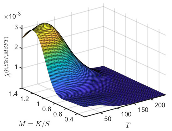
Figure 9. Implied information intensity against time to maturity T and moneyness $M=K/S$.

7. Conclusions

Inclusion of more information on market microstructure will inevitably lead to better option pricing models. As noted in the survey by Easley and O’Hara (2003), while “market microstructure and asset pricing models both consider the behavior and formation of prices in asset markets … neither literature explicitly recognizes the importance and role of the factors so crucial to the other approach." As an example of the separation in these two approaches, they contrast the conclusion that ‘reasonable stationarity assumptions in asset pricing theory lead to the expectation that price changes follow a random walk’ with a quote from Hasbrouk (1996) “At the level of transaction prices, …, the random walk conjecture is a straw man, a hypothesis that is very easy to reject in most markets even in small data samples. In microstructure, the question is not “whether” transaction prices diverge from a random walk, but rather “how much” and “why?”. In this paper, we have taken two steps to increase the amount of microstructure information included in a discrete, binomial option pricing model.

Using the Donsker–Prokhorov invariance principle, we extended the KSRF model to allow for variably-spaced trading instances, which, for example, is of critical importance to the short seller of an option. In particular we derive the expression for the discrete risk-neutral upturn probability $q_{n,k}$ for an arbitrarily spaced time period and quantify its dependence on the discrete, time-varying, natural-world upturn probability $p_{n,k}$. By reverting to a fixed-spaced trading interval (of 1 day), and using market data, we compare the relative behaviors of $q_{n,k}$ and $p_{n,k}$. We have also inferred the underlying natural probabilities $p_{\mathsf{\Delta }t}^{\left(\mathrm{CRR}\right)}$ and $p_{\mathsf{\Delta }t}^{\left(\mathrm{JR}\right)}$ that are missing from the Cox–Ross–Rubenstein and Jarrow–Rudd models and compare them with actual probabilities.

We employed the Cherny–Shiryaev–Yor invariance principle to construct option pricing within a complete market model in which the underlying stock dynamics depends on the (path-dependent) history of a market index (or market influencing factor). We add terms to the discrete log-return dynamics which, in the continuum limit, correspond to path-integrated volatility and a doubly-integrated volatility. A critical variable that emerges from this extension is ${\xi }_{n,k}^{\left(M\right)}$ defined in (14b), which depends on the upturn probability ${\mathsf{𝕡}}_{\mathsf{\Delta }t}$ of the underlying stock. The dynamics of ${\xi }_{n,k}^{\left(M\right)}$ and the added terms are investigated numerically in the Appendix A. As a result of the path dependence, the market price of risk, which drives the risk-neutral probability, is time-dependent, leading to a heavy-tailed distribution for the log-returns and potentially a more realistic pricing model for an option. Using numerical data, we explore the potential deviation between the price volatility of a call option based upon this new asset pricing approach and that provided by the CBOE. With reference to the first paragraph of this section, we note that, in our model based upon the Cherny–Shiryaev–Yor invariance principle, the discrete time dynamics of the stock prices does not follow a random walk, as the stock price is path dependent.

We explored the implications for option pricing under a market in which traders employ a statistical arbitrage strategy using forward contracts based upon their assumed knowledge of the market index upturn probability. In such a market, the market price of risk develops a drift term that now reflects the information intensity ${\lambda }^{(\aleph ,M)}$ of the traders. Using a numerical example, we explore the value of the information intensity of a call option as a function of moneyness and time to maturity. This example explicitly demonstrates that the market microstructure view—’in real markets, traders use information about stock price direction’—can, in fact, be incorporated within dynamic asset pricing theory. Thus, we believe that reconciling market microstructure and dynamic asset pricing is possible, and that one approach to doing so is through discrete-time pricing models. In particular, an idea suggested by Aït-Sahalia and Jacod (2014) to model microstructure dynamics as discrete semimartingales plus noise provides one plausible route.

References

- Aragon, George O., and Wayne E. Ferson. 2006. Portfolio performance evaluation. Foundations and Trends in Finance 2: 83–190. [Google Scholar] [CrossRef]
- Audrino, Francesco, Robert Huitema, and Markus Ludwig. 2019. An empirical implementation of the Ross Recovery Theorem as a prediction device. Journal of Financial Econometrics. [Google Scholar] [CrossRef]
- Aït-Sahalia, Yacine, and Jean Jacod. 2014. High-Frequency Financial Econometrics. Princeton: Princeton University Press. [Google Scholar]
- Billingsley, Patrick. 1962. Limit theorems for randomly selected partial sums. Annals of Mathematical Statistics 33: 85–92. [Google Scholar] [CrossRef]
- Billingsley, Patrick. 1999. Convergence of Probability Measures, 2nd ed. New York: Wiley-Interscience. [Google Scholar]
- Black, Fischer, and Myron Scholes. 1973. The pricing of options and corporate liabilities. Journal of Political Economy 81: 637–54. [Google Scholar] [CrossRef]
- Borisov, Igor Semenovich. 1984. On the rate of convergence in the Donsker-Prokhorov invariance principle. Theory of Probability and Its Applications 28: 388–93. [Google Scholar] [CrossRef]
- Boyle, Phelim P. 1986. Option valuation using a three-jump process. International Options Journal 3: 7–12. [Google Scholar]
- Boyle, Phelim P. 1988. A lattice framework for option pricing with two state variables. Journal of Financial and Quantitative Analysis 23: 1–12. [Google Scholar] [CrossRef]
- Breloer, Bernhard, Hannah Lea Hühn, and Hendrik Scholz. 2016. Jensen alpha and market climate. Journal of Asset Management 17: 195–214. [Google Scholar] [CrossRef]
- Carhart, Mark M. 1997. On persistence of mutual fund performance. Journal of Finance 52: 57–82. [Google Scholar] [CrossRef]
- Chen, Louis H.Y., Larry Goldstein, and Qi-Man Shao. 2011. Normal Approximation by Stein’s Method. Berlin: Springer. [Google Scholar]
- Cherny, Aleksander S., Albert N. Shiryaev, and Marc Yor. 2003. Limit behavior of the “horizontal-vertical” random walk and some extensions of the Donsker-Prokhorov invariance principle. Theory of Probability and Its Applications 47: 377–94. [Google Scholar] [CrossRef]
- Coleman, Thomas F., and Yuying Li. 1996. A reflective Newton method for minimizing a quadratic function subject to bounds on some of the variables. SIAM Journal on Optimization 6: 1040–58. [Google Scholar] [CrossRef]
- Coviello, Rosanna, Cristina Di Girolami, and Franesco Russo. 2011. On stochastic calculus related to financial assets without semimartingales. Bulletin Des Sciences Mathématiques 135: 733–74. [Google Scholar] [CrossRef]
- Cox, John C., Stephen A. Ross, and Mark Rubinstein. 1979. Options pricing: A simplified approach. Journal of Financial Economics 7: 229–63. [Google Scholar] [CrossRef]
- Crimaldi, Irene, Dai Pra Paolo, Pierre-Yves Louis, and Ida G. Minelli. 2019. Synchronization and functional central limit theorems for interacting reinforced random walks. Stochastic Processes and Their Applications 129: 70–101. [Google Scholar] [CrossRef]
- Davydov, Youri, and Vladimir Rotar. 2008. On a non-classical invariance principle. Statistics & Probability Letters 78: 2031–38. [Google Scholar]
- Delbaen, Freddy, and Walter Schachermayer. 1998. The fundamental theorem of asset pricing for unbounded stochastic processes. Mathematische Annalen 312: 215–50. [Google Scholar] [CrossRef]
- Dhaene, Jan, Ben Stassen, Pierre Devolder, and Michel Vellekoop. 2015. The minimal entropy martingale measure in a market of traded financial and actuarial risks. Journal of Computational and Applied Mathematics 282: 111–33. [Google Scholar] [CrossRef]
- Donsker, Monroe D. 1951. An invariant principle for certain probability limit theorems. Memoirs of the American Mathematical Society 6: 1–10. [Google Scholar]
- Dudley, Richard M. 1968. Distances of probability measures and random variables. Annals of Mathematical Statistics 39: 1563–72. [Google Scholar] [CrossRef]
- Dudley, Richard M. 2018. Real Analysis and Probablity. Boca Raton: CRC Press. [Google Scholar]
- Duffie, Darrell. 2001. Dynamic Asset Pricing Theory, 3rd ed. Princeton: Princeton University Press. [Google Scholar]
- Duffie, Darrell, and Henry R. Richardson. 1991. Mean-variance hedging in continuous time. The Annals of Applied Probability 1: 1–15. [Google Scholar] [CrossRef]
- Easley, David, and Maureen O’Hara. 2003. Microstructure and asset pricing. In Handbook of the Economics of Finance. Edited by G. M. Constantinides, M. Harris and R. M. Stulz. Amsterdam: Elsevier, vol. 1, pp. 1021–51. [Google Scholar]
- Esche, Felix, and Martin Schweizer. 2005. Minimal entropy preserves the Lévy property: How and why. Stochastic Processes and Their Applications 115: 299–27. [Google Scholar] [CrossRef]
- Fama, Eugene, and Kenneth French. 1993. Common risk factors in the returns on stocks and bonds. Journal of Financial Economics 33: 3–56. [Google Scholar] [CrossRef]
- Fama, Eugene, and Kenneth French. 2004. The capital asset pricing model: Theory and evidence. Journal of Economic Perspectives 18: 25–46. [Google Scholar] [CrossRef]
- Fama, Eugene, and Kenneth French. 2015. A five-factor asset pricing model. Journal of Financial Economics 116: 1–22. [Google Scholar] [CrossRef]
- Fama, Eugene, and Kenneth French. 2017. International tests of a five-factor asset pricing model. Journal of Financial Economics 123: 441–63. [Google Scholar] [CrossRef]
- Fischer, Hans. 2011. A History of the Central Limit Theorem. From Classical to Modern Probability Theory. New York: Springer. [Google Scholar]
- Florescu, Ionut, and Frederi G. Viens. 2008. Stochastic volatility: Option pricing using a multinomial recombining tree. Journal of Applied Mathematical Finance 15: 151–81. [Google Scholar] [CrossRef]
- Fortet, R., and E. Mourier. 1953. Convergence de la répartition empirique vers la répartition théorique. Annales Scientifiques de L’École Normale Supérieure 70: 267–85. [Google Scholar] [CrossRef]
- Fujiwara, Tsukasa, and Yoshio Miyahara. 2003. The minimal entropy martingale measures for geometric Lévy processes. Finance and Stochastics 7: 509–31. [Google Scholar] [CrossRef]
- Gikhman, Iosif I., and Anatoly V. Skorokhod. 1969. Introduction to the Theory of Random Processes. Philadephia: W.B. Saunders Company. [Google Scholar]
- Gut, Allan. 2009. Stopped Random Walks, 2nd ed. New York: Springer. [Google Scholar]
- Hasbrouk, Joel. 1996. Modeling microstructure time series. In The Handbook of Statistics. Edited by G. S. Maddala and C. R. Rao. Amsterdam: Elsevier, vol. 14, pp. 47–691. [Google Scholar]
- Hasbrouk, Joel. 2007. Empirical Market Microstructure. New York: Oxford Press. [Google Scholar]
- Hu, Yuan, Abootaleb Shirvani, Stoyan V. Stoyanov, Young Shin Kim, Frank J. Fabozzi, and Svetlozar T. Rachev. 2020. Option pricing in markets with informed traders. International Journal of Theoretical and Applied Finance. [Google Scholar] [CrossRef]
- Hull, John C. 2018. Options, Futures, and Other Derivatives, 10th ed. New York: Pearson. [Google Scholar]
- Jabbour, George M., Marat V. Kramin, Timur Kramin, and Stephen D. Young. 2005. Multinomial Lattices and Derivatives Pricing. In Advances in Quantitative Analysis of Finance and Accounting. Edited by C. -F. Lee. Singapore: World Scientific, vol. 2, pp. 1–17. [Google Scholar]
- Jackwearth, Jens C., and Marco Menner. 2020. Does the Ross recovery theorem work empirically? Journal of Financial Economics 137: 723–39. [Google Scholar] [CrossRef]
- Jacod, Jean, and Philip Protter. 2012. Discretization of Processes, Stochastic Modeling and Applied Probability. Heidelberg: Springer, vol. 67. [Google Scholar]
- Jarrow, Robert A., and Andrew Rudd. 1983. Option Pricing. Homewood: Richard D. Irwin. [Google Scholar]
- Jensen, Michael C. 1968. The performance of mutual funds in the period 1945–1964. Journal of Finance 23: 389–416. [Google Scholar] [CrossRef]
- Jensen, Michael C. 1969. Risk, the pricing of capital assets, and the evaluation of investment portfolios. Journal of Business 42: 167–247. [Google Scholar] [CrossRef]
- Johnson, R. Stafford, James Pawlukiewicz, and Jayesh Mehta. 1997. Binomial option pricing with skewed asset returns. Review of Quantitative Finance and Accounting 9: 89–101. [Google Scholar] [CrossRef]
- Kim, Young Shin, Stoyan V. Stoyanov, Svetlozar T. Rachev, and Frank J. Fabozzi. 2016. Multi-purpose binomial model: Fitting all moments to the underlying Brownian motion. Economics Letters 145: 225–29. [Google Scholar] [CrossRef]
- Kim, Young Shin, Stoyan V. Stoyanov, Svetlozar T. Rachev, and Frank J. Fabozzi. 2019. Enhancing binomial and trinomial option pricing models. Finance Research Letters 28: 185–90. [Google Scholar] [CrossRef]
- Madan, Dilip, Frank Milne, and Hersh Shefrin. 1989. The multinomial option pricing model and its Brownian and Poisson limits. Review of Financial Studies 2: 251–65. [Google Scholar] [CrossRef]
- Major, Péter. 1978. On the invariance principle for independent identically distributed random variables. Journal of Multivariate Analysis 8: 487–517. [Google Scholar] [CrossRef]
- Merton, Robert C. 1973. Theory of rational option pricing. Bell Journal of Economics and Management Science 4: 141–83. [Google Scholar] [CrossRef]
- O’Hara, Maureen. 1998. Market Microstructure Theory. Malden: Blackwell. [Google Scholar]
- Pesšta, Michal, and Ostap Okhrin. 2014. Conditional least squares and copulae in claims reserving for a single line of business. Mathematics and Economics 56: 28–37. [Google Scholar] [CrossRef]
- Prokhorov, Yuri V. 1956. Convergence of random processes and limit theorems in probability theory. Theory of Probability and its Applications 1: 157–14. [Google Scholar] [CrossRef]
- Rachev, Svetlozar T. 1985. The Monge-Kantorovich mass transference problem and its stochastic applications. Theory of Probability & Its Applications 29: 647–76. [Google Scholar]
- Rendleman, Richard J., and Brit J. Bartter. 1979. Two-state option pricing. Journal of Finance 34: 1093–110. [Google Scholar] [CrossRef]
- Ross, Stephen A. 2015. The recovery theorem. Journal of Finance 70: 615–48. [Google Scholar] [CrossRef]
- Rubinstein, Mark. 2000. On the relation between binomial and trinomial option pricing models. Journal of Derivatives 8: 47–50. [Google Scholar] [CrossRef]
- Senatov, Vladimir V. 2017. On the real accuracy of approximation in the central limit theorem. II. Siberian Advances in Mathematics 27: 133–52. [Google Scholar] [CrossRef]
- Sierag, Dirk, and Bernard Hanzon. 2018. Pricing derivatives on multiple assets: Recombining multinomial trees based on Pascal’s simplex. Annals of Operations Research 266: 101–27. [Google Scholar] [CrossRef]
- Silvestrov, Dmitrii S. 2004. Limit Theorems for Randomly Stopped Stochastic Processes. London: Springer. [Google Scholar]
- Skorokhod, Anatoliy V. 1956. Limit theorems for stochastic processes. Theory of Probability and its Applications 1: 261–90. [Google Scholar] [CrossRef]
- Skorokhod, Anatoliy V. 2005. Basic Principles and Applications of Probability Theory. Heidelberg: Springer. [Google Scholar]
- Tanaka, Katsuto. 2017. Time Series Analysis. Nonstationary and Noninvertible Distribution Theory, 2nd ed. Hoboken: Wiley. [Google Scholar]
- Whaley, Robert E. 2006. Derivatives: Markets, Valuation and Risk Management. Hoboken: Wiley. [Google Scholar]
- Yamada, Yuji, and James A. Primbs. 2004. Properties of multinomial lattices with cumulants for option pricing and hedging. Asia-Pacific Financial Markets 11: 335–65. [Google Scholar] [CrossRef]
- Yuen, Fei Lung, Tak Siu, and Hailiang Yang. 2013. Option valuation by a self-exciting threshold binomial model. Mathematical and Computer Modeling 58: 28–37. [Google Scholar] [CrossRef]