A Principal Component-Guided Sparse Regression Approach for the Determination of Bitcoin Returns

Theodore Panagiotidis; Thanasis Stengos; Orestis Vravosinos

doi:10.3390/jrfm13020033

,

and

¹

Department of Economics, University of Macedonia, Thessaloniki 54636, Greece

²

Department of Economics and Finance, University of Guelph, Guelph, ON N1G 2W1, Canada

³

Department of Economics, New York University, New York, NY 10003, USA

^*

Author to whom correspondence should be addressed.

J. Risk Financial Manag.2020, 13(2), 33;https://doi.org/10.3390/jrfm13020033

This article belongs to the Special Issue Recent Developments in Cryptocurrency Markets: Co-movements, Spillovers and Forecasting

Version Notes

Order Reprints

Abstract

We examine the significance of fourty-one potential covariates of bitcoin returns for the period 2010–2018 (2872 daily observations). The recently introduced principal component-guided sparse regression is employed. We reveal that economic policy uncertainty and stock market volatility are among the most important variables for bitcoin. We also trace strong evidence of bubbly bitcoin behavior in the 2017–2018 period.

Keywords:

bitcoin; cryptocurrency; bubble; sparse regression; LASSO; PC-LASSO; principal component; flexible least squares

JEL Classification:

G12; G15

1. Introduction

Introduced by (Nakamoto 2008), bitcoin is a digital currency with characteristics not found in traditional currencies; for example, it is not as robust a medium of exchange or store of value as traditional currencies. As outlined by (Panagiotidis et al. 2018a), it allows for transactions without bank intermediation or any transaction fees, and also offers anonymity. To get a sense of the pace in which the overall frequency of bitcoin transactions has been increasing, note that from less than 10,000 daily bitcoin transactions in the period 2011–2012, in 2019 there were around 300,000 bitcoin transactions per day.1

We examine the potential covariates of bitcoin returns (e.g., stock market returns, stock market volatility, exchange rates, commodities, central bank rates, internet trends and policy uncertainty). (Panagiotidis et al. 2018a) have also considered a variety of potentially important variables for bitcoin returns (21 variables in total, whereas here we consider 41) employing the least absolute shrinkage and selection operator (LASSO).2 We examine a larger set of potential variables (41) and account for the group structure of the independent variables.

We employ the principal component-guided sparse regression (PC-LASSO) introduced by (Tay et al. 2018) to identify the variables that are most important for bitcoin. This procedure allows us to consider numerous potential variables (41 in our case) and select only a subset of the covariates (as standard LASSO does). We thus consider far more variables possibly important for bitcoin than in earlier studies (e.g., (Panagiotidis et al. 2018a, 2018b)). PC-LASSO also exploits the correlation and the group structure of the independent variables by shrinking each group-wise component of the solution towards the leading principal components of that group (e.g., the group of stock market returns variables), which is not the case for standard LASSO employed in (Panagiotidis et al. 2018a).3 Doing so yields results contradicting some of those in (Panagiotidis et al. 2018a, 2018b). Next, we perform a rolling-window PC-LASSO estimation to gauge how the interactions of alternate variables with bitcoin have changed over time. Last, we examine their variability by keeping only the variables surviving the PC-LASSO (i.e., that have non-zero coefficients) and employing the flexible least squares (FLS) methodology of (Kalaba and Tesfatsion 1989). The rest of the paper is organized as follows: Section 2 presents the data and methods used, Section 3 discusses the results and the last section concludes.

2. Methods and Data

We use daily (7-day week) data for the period spanning from 21 July 2010 to 31 May 2018 (2872 observations). Most of the data come from Thomson Reuters Eikon, while for bitcoin the Coindesk Bitcoin Price Index (BPI) is used. Wikipedia trend data were retrieved using the package “wikipediatrend” till the 21 January 2016 (they were not available after this date). More recent data were filled from tools.wmflabs.org.4 The reader is referred to Table A1 in the Appendix B for a complete list of the independent variables considered.

The variables that are not of daily frequency or are of a 5-day per week frequency have been linearly interpolated.5 Variables were used in levels or first differences depending on their stationary characteristics.6 For comparability of the coefficients, all variables were standardized to have mean 0 and a variance of 1. As in (Forbes and Rigobon 2002), we accounted for differences in opening hours of the stock markets by using 2-day rolling averages for stock-market specific variables.

Similar to (Panagiotidis et al. 2018a), we considered the full sample, as well as three sub-periods of it separately: (1) 21 July 2010–10 December 2013, (2) 11 December 2013–24 March 2017 and (3) 25 March 2017–31 May 2018. The selection of these three periods was motivated by (1) the different phases the bitcoin market has been through and (2) the rolling window generalized supremum Augmented Dickey–Fuller test for bubbles (GSADF; (Phillips et al. 2015)) (see Figure A1 in the Appendix B).7 The first period reflects the early phase of bitcoin with lower traded quantities including the first bitcoin boom in late 2013 and Mt. Gox’s suspension of trading and filing for bankruptcy protection. The second is a period of higher stability and gradual recovery, while the third one corresponds to the recent alleged bubble.8 The selection of the break points is corroborated by the sub-periods obtained in (Panagiotidis et al. 2018a) under different methods; namely, an ADF breakpoint unit root test.

We estimate PC-LASSO models for each of the three periods and the entire sample.9 This is done with two alternative approaches: first with the principal component (PC) groups defined by different market/factor types (i.e., stock market returns, policy uncertainty), and second, with the PC groups defined by geographical region (i.e., US, Europe etc.). PC-LASSO admits overlapping PC groups, which allows us to ascribe variables to two different geographical regions when necessary. With the first approach for PC grouping, we gain insight on which variables are the most important for bitcoin within each market/factor type, while with the second which variables are the most significant within each geographical region. Next, we perform a rolling-window PC-LASSO estimation to gauge how the sign and the importance of the interaction of alternate variables with bitcoin has changed over time.

(Tay et al. 2018) described PC-LASSO as a method for supervised learning combining the LASSO sparsity penalty with a quadratic penalty that shrinks the coefficient vector toward the leading principal components of the independent variables. When the independent variables can be grouped to different categories, they shrink each group-wise component of the solution toward the leading principal components of that group. PC-LASSO is discussed in Appendix A.

Using the variables that have a non-zero coefficient in the PC-LASSO with market/factor type PC groups for the full sample, we estimate a time-varying linear regression employing the FLS approach of (Kalaba and Tesfatsion 1989) with Kalman filtering and check the robustness of the results using a standard state-space approach where coefficients are treated as separate random walks.10

Table 1 summarizes the approaches employed in the paper.

Table 1. Summary of methods used.

3. Results

In line with (Panagiotidis et al. 2018a, 2018b), variables such as economic policy uncertainty and stock market volatility emerge as the most important ones featuring a negative relation with bitcoin. We find foreign exchange (FX) markets, monetary policy and popularity measures to be of relatively minor importance. More profound was the effect of traditional stock market returns corroborating the evidence in (Panagiotidis et al. 2018a). The US stock market emerges as the most important one—in terms of both volatility and returns: the positive relationship with the US stock market returns and the negative one with volatility point to some degree of connection between bitcoin and traditional financial markets. Interestingly, even though popularity measures (i.e., Google and Wikipedia article access trends) appear not to be significant overall, in the second sub-period—that is, after the first bitcoin boom and Mt. Gox’s suspension of trading and filing for bankruptcy protection—both variables are negatively related to bitcoin returns. This contradicts the results of (Panagiotidis et al. 2018a, 2018b) who found a positive and more pronounced consistent link between Google trends and bitcoin returns. Still in contrast to these results, we find gold not to play a role, which also holds for the other commodities considered. Additionally, EU monetary policy only appears to have played a role at the early stages of the European debt crisis, while their results suggested a stronger role of the European Central Bank (ECB) rate. Last, government bond yields seem to matter for bitcoin.

Table 2 presents the PC-LASSO coefficients for the full sample and for each of the three sub-periods separately when PC groups are formed by market/factor type. The Chicago Board Options Exchange (CBOE) volatility index is the most important, suggesting that among the US, Europe and Japanese stock markets, the volatility of the US one is the most significant for bitcoin.

Table 2. PC-LASSO with market/factor type components’ coefficients of independent variables.

Table 3 presents the PC-LASSO coefficients for the full sample and for each of the three sub-periods separately when PC groups are formed by geographic region. Again, the CBOE volatility index appears to be among the most relevant variables for bitcoin and among the US variables. Russia’s economic policy uncertainty (EPU) is, with both PC groupings, negatively associated to bitcoin returns. Notice also that in the first era of bitcoin, economic policy uncertainty was crucial for bitcoin. Last, under both PC groupings, all variables but the US Fed Funds effective rate (FFER) have a zero coefficient in the most recent period. This combined with the GSADF statistic (Figure A1) serves as signal of bubbly behavior in the period 2017-2018 with bitcoin weakly connected to the markets and following its own—arguably irregular—path. The GSADF also provides evidence of a bubble during the bicoin boom of 2013 before the Mt. Gox trading suspension and filing for bankruptcy protection.

Table 3. PC-LASSO with geographic region components coefficients of independent variables.

Figure 1 presents the rolling window PC-LASSO coefficient estimates (with market/factor type components) for the ten independent variables whose coefficients are non-zero the most times in the rolling window estimation.11 Three of the ten variables are related to uncertainty (two economic policy uncertainty and one stock market uncertainty), three to stock market returns and two to internet trends. Notice that both in the early phase of lower traded quantities and the first bitcoin boom and in the third one we have identified, corresponding to the recent alleged bubble, the coefficients of Google and Wikipedia trends are generally positive (or zero), while in the middle phase (of the burst of the first boom and following Mt. Gox’s suspension of trading and filing for bankruptcy protection), the coefficients turn more negative. This points to the capability of internet trends to accelerate the creation and the burst of a bubble.12

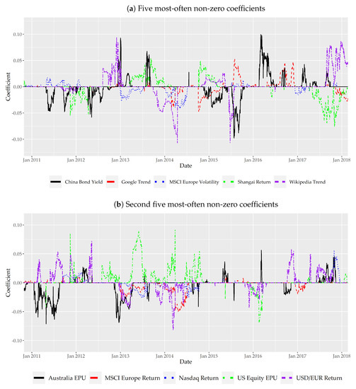
Figure 1. Rolling window PC-LASSO coefficients with market/factor type components. Notes: The window size is 200 observations. All variables are standardized in each window separately. For comparability λ = 15 and r = 0.7 across all windows. The ECB the Chinese central bank rates have not been included in the analysis, as they often do not vary within windows. The coefficients on a given date correspond to the window whose 100th observation corresponds to that date. In the first panel are the coefficients of the five independent variables whose coefficients are most often non-zero in the rolling window estimation (for example, the China bond yield is the variable whose coefficient is non-zero the most times; that is, in 994 out of the 2673 rolling window estimations); in the second panel are the five variables with the next highest numbers of non-zero coefficients. Morgan Stanley Capital International’s (MSCI) Europe volatility index and the USD/EUR return have equal numbers of non-zero coefficients (892).

4. Conclusions

In this study we examined fourty-one potential drivers of bitcoin returns for the period 2010–2018, including stock market returns, stock market volatility, exchange rates, commodities, central bank rates, internet trends and policy uncertainty. We split the sample into the three different phases the bitcoin market has been through based also on the rolling window GSADF test for bubbles (Phillips et al. 2015). Employing the principal component-guided sparse regression (PC-LASSO) recently introduced by (Tay et al. 2018), we identified the variables that are most important for bitcoin. Furthermore, after selecting a subset of the examined variables based on the PC-LASSO results, we employed the flexible least squares (FLS) methodology of (Kalaba and Tesfatsion 1989) to gauge how the importance of alternate variables for bitcoin has changed over time.

We found that variables such as economic policy uncertainty and stock market volatility are among the most important ones for bitcoin. We also traced strong evidence of bubbly bitcoin behavior, especially in the 2017–2018 period, as well as evidence that internet trends can expedite the creation and the burst of a bubble. We found a minor importance for FX markets and monetary policy, but a higher one for traditional stock market returns. Commodity markets appear not to play a role, while the opposite holds for government bond yields.

Author Contributions

The authors have contributed to this work as follows: conceptualization, T.P., T.S. and O.V.; methodology, T.P., T.S., O.V.; data work, O.V.; writing—review and editing, T.P. and O.V. All authors have read and agreed to the published version of the manuscript.

Funding

This research received no external funding.

Conflicts of Interest

The authors declare no conflict of interest.

Appendix A. The PC-LASSO Methodology

This section follows (Tay et al. 2018). Let

Y

and

X

be the vector and matrix of the dependent and the independent variables with centered columns, respectively. Additionally, let the p potential predictors of bitcoin be grouped in K non-overlapping groups. For

k = 1, \dots, K

X_{k}

denotes the

p_{k}

columns of

X

corresponding to group k,

m_{j} : = rank (X_{k})

and

(V_{k}, d_{k})

denotes the right singular vectors and singular values of

X_{k}

. PC-LASSO minimizes:

\begin{matrix} J (β) = \frac{1}{2} {∥y - X β∥}_{2}^{2} + λ {∥β∥}_{1} + \frac{θ}{2} \sum_{k} β_{k}^{T} (V_{k} D_{d_{k 1}^{2} - d_{k j}^{2}} V_{k}^{T}) β_{k}, \end{matrix}

where

β_{k}

is the sub-vector of

β

corresponding to group k,

d_{k} = (d_{k 1}, \dots, d_{k m})

are the singular values of

X_{k}

in decreasing order and

D_{d_{k 1}^{2} - d_{k j}^{2}}

is a diagonal matrix with diagonal entries

d_{k 1}^{2} - d_{k j}^{2}

for

j = 1, \dots, m_{k}

.

θ

and

λ

are parameters to be chosen, often through cross-validation. PC-LASSO gives:

X \hat{β} = \sum_{j = 1}^{m} \frac{d_{j}^{2}}{d_{j}^{2} + θ (d_{1}^{2} - d_{j}^{2}) u_{j} u_{j}^{T} y}

(A1)

where

m : = rank (X)

;

u_{j}

the j-th column of the matrix

U

, where

U D V^{T}

the singular value decomposition of

X

; and

d_{1} \geq d_{2} \geq \dots \geq d_{m} > 0

the diagonal entries of the diagonal matrix

D

.

d_{j}^{2} /[d_{j}^{2} + θ (d_{1}^{2} - d_{j}^{2}) u_{j} u_{j}^{T} y]

is called the shrinkage factor.

The objective function can be optimized efficiently by a coordinate descent procedure, since it is convex and the non-smooth component is separable. As the parameter

θ

is difficult to interpret, one can specify the ratio r between the shrinkage factors in Equation (A1) for

k = 2

and

k = 1

(the latter being equal to 1). The admissible range for the ratio is

[0, 1]

, where 1 corresponds to

θ = 0

(standard LASSO) and lower values induce stronger shrinkage.

Appendix B. Data Description and Supplementary Results

Table A1. Variables employed, sample: June 21st 2010 to May 31st 2018 (7-day week; 2872 observations).

Variable	Market/Factor Type	Region	Eikon Code
Crude Oil-WTI Spot Cushing (in USD/BBL)	Commodities market returns	World	CRUDOIL
MLCX - Gas oil Spot Index - price index	Commodities market returns	World	MLCXQSS
S&P GSCI Gold Total Return	Commodities market returns	World	GSGCTOT
DJGL World - price index	Equity market returns	World	DJWRLD$
Dow Jones 65 Composite Average - price index	Equity market returns	US	DJCMP65
MSCI Europe - price index	Equity market returns	Europe	MSEROP$
Nasdaq Composite - price index	Equity market returns	US	NASCOMP
Nikkei 225 Psychological - price index	Equity market returns	Asia	JAPDOWP
Nikkei 225 Stock Average - price index	Equity market returns	Asia	JAPDOWA
S&P 500 Composite - price index	Equity market returns	US	S&PCOMP
Shangai SE Composite - price index	Equity market returns	Asia	CHSCOMP
CBOE SPX Volatility VIX - price index	Equity market volatility	US	CBOEVIX
Euro Stoxx 50 Volatility Index - price index	Equity market volatility	Europe	VST1MEI
MSCI Europe Minimum Volatility (in USD) - price index	Equity market volatility	Europe	MSURMV$
Nikkei Stock Average Volatility Index - price index	Equity market volatility	Asia	VXJINDX
Chinese Yuan to USD (WMR) – exchange rate	FX market returns	US/Asia	CHIYUA$
Japanese Yen to USD (WMR) – exchange rate	FX market returns	US/Asia	JAPAYE$
USD to Euro (WMR&DS) – exchange rate	FX market returns	US/Europe	USEURSP
USD to UK pound (WMR) – exchange rate	FX market returns	US/Europe	USDOLLR
China Government Benchmark Bid Yield - 10 Years	Government bond yields	Asia	TRCH10T
Japan Government Benchmark Bid Yield - 10 Years	Government bond yields	Asia	TRJP10T
US Government Benchmark Bid Yield - 10 Years	Government bond yields	US	TRUS10T
Google Trend for the term ‘’bitcoin’’	Investor attention	World	-
Wikipedia trend for the article on bitcoin	Investor attention	World	-
Euro Overnight Deposit (ECB) – middle rate	Monetary policy	Europe	EURODEP
Japan Uncollateralized Overnight – middle rate	Monetary policy	Asia	JPCALLO
Chinese Renminbi 1D Notice Deposit – middle rate	Monetary Policy	Asia	CHDEPCL
US Fed Funds Effective Rate – middle rate	Monetary policy	US	FRFEDFD
Australia Economic Policy Uncertainty Index (news based)	Policy uncertainty	Australia	AUEPUNEWR
China Economic Policy Uncertainty Index (news based)	Policy uncertainty	Asia	CHEPUNEWR
EU Economic Policy Uncertainty Index (news based)	Policy uncertainty	Europe	EUEPUNEWR
India Economic Policy Uncertainty Index (news based)	Policy uncertainty	Asia	INEPUNEWR
Japan Economic Policy Uncertainty Index (news based)	Policy uncertainty	Asia	JPEPUOVAR
Russia Economic Policy Uncertainty Index (news based)	Policy uncertainty	Europe/Asia	RSEPUNEWR
Singapore Economic Policy Uncertainty Index (news based)	Policy uncertainty	Asia	SPEPUTWAR
South Korea Economic Policy Uncertainty Index (news based)	Policy uncertainty	Asia	KOEPUOVAR
UK Economic Policy Uncertainty Index	Policy uncertainty	Europe	UKEPUPO
US Economic Policy Uncertainty Index (news based)	Policy uncertainty	US	USEPUNEWR
US Economic Policy Uncertainty Index	Policy uncertainty	US	USEPUPO
US Equity-related Economic Policy Uncertainty Index	Policy uncertainty	US	USEPUEQ
World Economic Policy Uncertainty Index – PPP-adj	Policy uncertainty	World	WDEPUPPPR

In Figure A2, panel (a) presents the FLS coefficient paths for the independent variables whose coefficients vary out of the thirteen variables with non-zero coefficients in the full sample column of Table 2 included in the model. The ECB overnight deposit rate appears significant in the beginning of the European debt crisis, in which period Europe stock market volatility also seems to have increased importance. Additionally, the US equity-related EPU appears constantly significant across the examined period. Panel (b) presents analogous results for a lower smoothing parameter value along with the coefficient paths under a standard state-space approach with Kalman filtering where coefficients are treated as separate random walks. The paths for the coefficients that vary over time are similar in the two methods.

Figure A1. Coindesk BPI and the generalized sup augmented Dickey–Fuller statistic. Notes: The final GSADF statistic is the largest ADF statistic, which in the figure is above 16. The asymptotic

99 %

critical value for an initial window

5.5 %

(ours is

3.5 %

) of the total sample is

2.74

based on numerical simulations with 2000 replications (Phillips et al. 2015). Given that the test statistic exceeds this value in some point (actually multiple) in the sample, there is evidence of bubbly behavior. The corresponding asymptotic critical value for the supremum ADF (SADF) tests constituting the GSADF test is 2.06, providing evidence of multiple cases of bubbles.

Figure A1. Coindesk BPI and the generalized sup augmented Dickey–Fuller statistic. Notes: The final GSADF statistic is the largest ADF statistic, which in the figure is above 16. The asymptotic

99 %

critical value for an initial window

5.5 %

(ours is

3.5 %

) of the total sample is

2.74

based on numerical simulations with 2000 replications (Phillips et al. 2015). Given that the test statistic exceeds this value in some point (actually multiple) in the sample, there is evidence of bubbly behavior. The corresponding asymptotic critical value for the supremum ADF (SADF) tests constituting the GSADF test is 2.06, providing evidence of multiple cases of bubbles.

Figure A2. Flexible least squares and state-space varying coefficient paths. (a) Flexible least squares with Kalman filtering varying coefficient paths. (b) Flexible least squares with Kalman filtering (in blue solid lines) and state-space with Kalman filtering (in red dashed lines) varying coefficient paths. Notes: In panel (a) the smoothing parameter has been set to 1; ±2 standard deviation bands are in light blue. In panel (b) the smoothing parameter for the FLS has been set to 0.1.

References

Aalborg, Halvor Aarhus, Peter Molnár, and Jon Erik de Vries. 2019. What can explain the price, volatility and trading volume of bitcoin? Finance Research Letters 29: 255–65. [Google Scholar] [CrossRef]
Biais, Bruno, Christophe Bisière, Matthieu Bouvard, Catherine Casamatta, and Albert J. Menkveld. 2018. Equilibrium Bitcoin Pricing. Available online: https://ssrn.com/abstract=3261063 (accessed on 7 February 2020). [CrossRef]
Caspi, Itamar. 2017. Rtadf: Testing for bubbles with eviews. Journal of Statistical Software, Code Snippets 81: 1–16. [Google Scholar] [CrossRef]
Corbet, Shaen, Brian Lucey, and Larisa Yarovaya. 2018. Datestamping the Bitcoin and Ethereum bubbles. Finance Research Letters 26: 81–88. [Google Scholar] [CrossRef]
Forbes, Kristin J., and Roberto Rigobon. 2002. No contagion, only interdependence: Measuring stock market comovements. Journal of Finance 57: 2223–61. [Google Scholar] [CrossRef]
Goczek, Ł, and I. Skliarov. 2019. What drives the bitcoin price? A factor augmented error correction mechanism investigation. Applied Economics 51: 6393–410. [Google Scholar] [CrossRef]
Hotz-Behofsits, Christian, Florian Huber, and Thomas Otto Zörner. 2018. Predicting crypto-currencies using sparse non-Gaussian state space models. Journal of Forecasting 37: 627–40. [Google Scholar] [CrossRef]
Jin, J., J. Yu, Y. Hu, and Y. Shang. 2019. Which one is more informative in determining price movements of hedging assets? Evidence from bitcoin, gold and crude oil markets. Physica A: Statistical Mechanics and its Applications 527: 121121. [Google Scholar] [CrossRef]
Kalaba, R., and L. Tesfatsion. 1989. Time-varying linear regression via flexible least squares. Computers & Mathematics with Applications 17: 1215–45. [Google Scholar] [CrossRef]
Kapetanios, George, and Filip Zikes. 2018. Time-varying Lasso. Economics Letters 169: 1–6. [Google Scholar] [CrossRef]
Kjærland, Frode, Aras Khazal, Erlend A. Krogstad, Frans B. G. Nordstrøm, and Are Oust. 2018. An analysis of bitcoin’s price dynamics. Journal of Risk and Financial Management 11: 63. [Google Scholar] [CrossRef]
Li, Jiahan, and Weiye Chen. 2014. Forecasting macroeconomic time series: LASSO-based approaches and their forecast combinations with dynamic factor models. International Journal of Forecasting 30: 996–1015. [Google Scholar] [CrossRef]
Nakamoto, Satoshi. 2008. Bitcoin: A Peer-to-Peer Electronic Cash System. Available online: https://bitcoin.org/bitcoin.pdf (accessed on 7 February 2020).
Panagiotidis, Theodore, Thanasis Stengos, and Orestis Vravosinos. 2018a. On the determinants of bitcoin returns: A LASSO approach. Finance Research Letters 27: 235–40. [Google Scholar] [CrossRef]
Panagiotidis, Theodore, Thanasis Stengos, and Orestis Vravosinos. 2018b. The effects of markets, uncertainty and search intensity on bitcoin returns. International Review of Financial Analysis 63: 220–42. [Google Scholar] [CrossRef]
Phillips, Peter C. B., Shuping Shi, and Jun Yu. 2015. Testing for multiple bubbles: Limit theory of real-time detectors. International Economic Review 56: 1079–134. [Google Scholar] [CrossRef]
Phillips, Peter C. B., Yangru Wu, and Jun Yu. 2011. Explosive Behavior In The 1990s Nasdaq: When Did Exuberance Escalate Asset Values?*. International Economic Review 52: 201–26. [Google Scholar] [CrossRef]
Schilling, Linda, and Harald Uhlig. 2019. Some simple bitcoin economics. Journal of Monetary Economics 106: 16–26. [Google Scholar] [CrossRef]
Tay, J. Kenneth, Jerome Friedman, and Robert Tibshirani. 2018. Principal component-guided sparse regression. arXiv arXiv:1810.04651. [Google Scholar]
Tibshirani, Robert. 1996. Regression shrinkage and selection via the lasso. Journal of the Royal Statistical Society: Series B (Methodological) 58: 267–88. [Google Scholar] [CrossRef]

1.	See https://www.blockchain.com/en/charts/n-transactions?timespan=all.
2.	There is a large literature testing for the importance of different variables for bitcoin. See for example (Kjærland et al. 2018; Aalborg et al. 2019; Goczek and Skliarov 2019; Jin et al. 2019). For a review of such literature see (Panagiotidis et al. 2018a).
3.	While standard LASSO has been around for more than two decades since it was introduced by (Tibshirani 1996), PC-LASSO was not available at the time of (Panagiotidis et al. 2018a’s) work.
4.	Due to discrepancies in the data and different scales of the two sources, a simple linear regression was estimated for the time period for which data from both sources was available, and Wikipedia trend values from 21 January and on were estimated using the values from tools.wmflabs.org.
5.	Google does not provide trend data in daily frequency for large time periods. Thus, for higher precision, daily Google trend data were obtained in nine-month intervals; then, log differences were computed and the values for the missing observations every nine months were interpolated.
6.	All variables were found to be I(0). Unit root tests are available upon request.
7.	GSADF is implemented in Eviews (Caspi 2017). Although in their empirical application (Phillips et al. 2015) used the S&P 500 stock price index and the real S&P 500 stock price index dividend data to implement the test on the price–dividend ratio, in our case it is hard to argue for any (measure of) fundamental value of bitcoin, so we implemented the test on bitcoin alone. This approach is most valid if the fundamental value of bitcoin is constant across time. For example, following a standard approach of the macroeconomic literature, (Schilling and Uhlig 2019) developed a model of an endowment economy with infinitely-lived agents and two intrinsically worthless currencies, a currency supplied by a central bank trying to achieve its inflation target, and bitcoin, whose supply grows deterministically. On the other hand, in the overlapping generations model with investors, miners and hackers (Biais et al. 2018) of the fundamental value of the cryptocurrency is the stream of net transactional benefits it will provide, which depend on its future prices. Looking into the fundamental drivers of the Bitcoin and Ethereum price, (Corbet et al. 2018) tested for the existence and dates of pricing bubbles employing the earlier methodology introduced in (Phillips et al. 2011).
8.	See for example https://www.ft.com/content/ce3ef54e-371b-11e7-bce4-9023f8c0fd2e?mhq5j=e1, https://www.ft.com/content/b5d66ed8-d1b3-11e6-b06b-680c49b4b4c0?mhq5j=e1, and https://www.ft.com/content/a2c5f07e-dbf9-11e7-a039-c64b1c09b482.
9.	We implement PC-LASSO using the R package “pcLasso”. (Hotz-Behofsits et al. 2018) test the forecasting performance of sparse state space models using a limited number of predictors.
10.	The FLS and state-space methods are implemented using the add-in "tvpuni" in Eviews. For the results, see Appendix B.
11.	Rolling window LASSO estimation has been employed by (Li and Chen 2014), while (Kapetanios and Zikes 2018) present an alternative methodology for time-varying Lasso estimation. Both of these are based on standard LASSO methods not exploiting the correlation and group structure of the independent variables through principal component guidance.
12.	Similar evidence is traced in the results in Table 2 and Table 3.

Figure 1. Rolling window PC-LASSO coefficients with market/factor type components. Notes: The window size is 200 observations. All variables are standardized in each window separately. For comparability λ = 15 and r = 0.7 across all windows. The ECB the Chinese central bank rates have not been included in the analysis, as they often do not vary within windows. The coefficients on a given date correspond to the window whose 100th observation corresponds to that date. In the first panel are the coefficients of the five independent variables whose coefficients are most often non-zero in the rolling window estimation (for example, the China bond yield is the variable whose coefficient is non-zero the most times; that is, in 994 out of the 2673 rolling window estimations); in the second panel are the five variables with the next highest numbers of non-zero coefficients. Morgan Stanley Capital International’s (MSCI) Europe volatility index and the USD/EUR return have equal numbers of non-zero coefficients (892).

Table 1. Summary of methods used.

Method	Details—Specifications
GSADF	Initial window size: 100 obs; intercept and trend included in the equation; number of lags in the test equation selected based on the Schwarz information criterion (with maximum allowed 7)
PC-LASSO	Dependent variable distribution: Gaussian; $r = 0.7$ ; principal component groups as given in the market/factor type column (Table 2 results) or in the region column (Table 3 results) of Table A1; $λ$ selected through 30-fold cross validation (that is, by repeated estimations of the model in subsamples of the total sample and making out-of-sample predictions, we find which value of $λ$ leads to better predictions on average); standardized variables; convergence threshold for coordinate descent algorithm: $10^{- 4}$
Rolling window PC-LASSO	Dependent variable distribution: Gaussian; $r = 0.7$ ; $λ = 15$ ; window size: 200obs.; principal component groups as given in the market/factor type column of Table A1; variables standardized in each window separately so that they are comparable within each time window; convergence threshold for coordinate descent algorithm: $10^{- 4}$
FLS	Flexible Least Squares (Kalaba and Tesfatsion 1989) and state-space models with Kalman filtering; smoothing parameter set equal to 1/0.1

Note: GSADF and PC-LASSO have been proposed by (Phillips et al. 2015; Tay et al. 2018), respectively.

Table 2. PC-LASSO with market/factor type components’ coefficients of independent variables.

Variable	Full Sample	1st Period	2nd Period	3rd Period
CBOE SPX Volatility VIX	−0.0358	−0.0290	0.0000	0.0000
US Equity-related EPU	0.0242	0.0010	0.0000	0.0000
Russia EPU	−0.0228	−0.0062	0.0000	0.0000
Australia EPU	−0.0215	−0.0488	0.0000	0.0000
Japan Government Benchmark Bid Yield	0.0170	0.0000	0.0000	0.0000
S&P 500 Composite 2-day return	0.0114	0.0098	0.0000	0.0000
US Government Benchmark Bid Yield	0.0026	0.0000	0.0000	0.0000
South Korea EPU	0.0020	0.0000	0.0000	0.0000
ECB Overnight Deposit Rate	0.0019	0.0000	0.0000	-
MSCI Europe Minimum Volatility Index	0.0015	0.0000	0.0000	0.0000
Google Trend log difference	0.0010	0.0000	−0.0102	0.0000
Euro Stoxx 50 Volatility Index	0.0008	0.0000	0.0000	0.0000
Nikkei Stock Average Volatility Index	−0.0004	−0.0026	0.0000	0.0000
Dow Jones 65 Composite 2-day return	0.0000	0.0002	0.0000	0.0000
US FFER	0.0000	0.0000	0.0000	−0.0074
India EPU	0.0000	−0.0023	0.0000	0.0000
Nikkei 225 Psychological Index	0.0000	−0.0071	0.0032	0.0000
China Government Benchmark Bid Yield	0.0000	0.0015	−0.0263	0.0000
US EPU	0.0000	−0.0046	0.0000	0.0000
USD/UK pound return	0.0000	0.0000	−0.0049	0.0000
Wikipedia trend log difference	0.0000	0.0000	−0.0026	0.0000
Cross-validation $λ$	39	21.06	56.42	53.87

Notes: The Chinese central bank rate does not vary in the 2nd and 3rd periods and the ECB rate does not vary in the 3rd period, so they have been excluded in the corresponding periods. Otherwise, all variables have been included in the regressions but the ones whose coefficients are zero in all three periods are not presented in the table. Principal component groups are as in the market/factor type column of Table A1. λ for the total sample has been selected through cross-validation. Cross-validation has also been performed for each of the three sub-periods, and then, for comparability, the average of the three resulting λs has been used for all three sub-periods. The variables have been standardized in the full sample and each sub-period separately. Due to the penalties used in the estimation, the method gives no confidence intervals for the coefficients.

Table 3. PC-LASSO with geographic region components coefficients of independent variables.

Variable	Full Sample	1st Period	2nd Period	3rd Period
Russia EPU	−0.0032	−0.0075	0.0000	0.0000
CBOE SPX Volatility VIX	−0.0024	−0.0097	0.0000	0.0000
S&P 500 Composite 2-day return	0.0001	0.0040	0.0000	0.0000
Australia EPU	0.0000	−0.0164	0.0000	0.0000
Dow Jones 65 Composite 2-day return	0.0000	0.0025	0.0000	0.0000
US FFER	0.0000	0.0000	0.0000	−0.0010
Google Trend log difference	0.0000	0.0000	−0.0094	0.0000
India EPU	0.0000	−0.0099	0.0000	0.0000
Japan Uncollateralized Overnight Rate	0.0000	0.0000	−0.0003	0.0000
Japan EPU	0.0000	−0.0095	0.0000	0.0000
Nikkei Stock Average Volatility Index	0.0000	−0.0043	0.0000	0.0000
Singapore EPU	0.0000	−0.0042	0.0000	0.0000
China Government Benchmark Bid Yield	0.0000	0.0005	−0.0025	0.0000
Japan Government Benchmark Bid Yield	0.0000	0.0000	−0.0006	0.0000
US EPU	0.0000	−0.0050	0.0000	0.0000
USD/UK pound return	0.0000	0.0000	−0.0002	0.0000
Cross-validation $λ$	98.89	21.06	81.86	53.87

Notes: The Chinese central bank rate does not vary in the 2nd and 3rd periods and the ECB rate does not vary in the 3rd period, so they have been excluded in the corresponding periods. Otherwise, all variables have been included in the regressions but the ones whose coefficients are zero in all three periods are not presented in the table. Principal component groups are as in the region column of Table A1. Australia is grouped with Asia and the five variables ascribed to two regions are included in the groups of both regions.

λ

for the total sample has been selected through cross-validation. Cross-validation has also been performed for each of the three sub-periods, and then, for comparability, the average of the three resulting

λ

s has been used for all three sub-periods. The variables have been standardized in the full sample and each sub-period separately. Due to the penalties used in the estimation, the method gives no confidence intervals for the coefficients.

© 2020 by the authors. Licensee MDPI, Basel, Switzerland. This article is an open access article distributed under the terms and conditions of the Creative Commons Attribution (CC BY) license (http://creativecommons.org/licenses/by/4.0/).

A Principal Component-Guided Sparse Regression Approach for the Determination of Bitcoin Returns

Abstract

1. Introduction

2. Methods and Data

3. Results

4. Conclusions

Author Contributions

Funding

Conflicts of Interest

Appendix A. The PC-LASSO Methodology

Appendix B. Data Description and Supplementary Results

References

Article Metrics

Citations

Article Access Statistics