Sample Path Generation of the Stochastic Volatility CGMY Process and Its Application to Path-Dependent Option Pricing

Abstract

This paper proposes the sample path generation method for the stochastic volatility version of the CGMY process. We present the Monte-Carlo method for European and American option pricing with the sample path generation and calibrate model parameters to the American style S&P 100 index options market, using the least square regression method. Moreover, we discuss path-dependent options, such as Asian and Barrier options.

1. Introduction

Lévy process models have played a role as the standard framework for option pricing, since these models allow for stochastic volatility and the volatility smile effect observed for the Black Scholes model (Black and Scholes (1973)). For instance, Hurst et al. (1999) applied an $\alpha$-stable process, Carr et al. (2002) used the Carr, Geman, Madan, and Yor (CGMY) process, which is a subclass of the tempered stable process (Rosiński 2007), and Bianchi et al. (2010) presented the tempered, infinitely divisible model. Moreover, Lévy process models with time-varying volatility have been used for option pricing in discrete time models, since empirical studies show that Brownian motion is often rejected (see Rachev and Mittnik (2000), Kim et al. (2010), Kim et al. (2011)). Carr et al. (2003) defined the class of continuous time stochastic volatility models on Lévy processes (SVLP) using the time-changed Lévy process. The SVLP model has been successfully applied in European option pricing, but the absence of an efficient sample path generation method makes the SVLP model hard to apply to path-dependent options, such as American, Barrier, or Asian options.

This paper proposes a sample path generation method for the stochastic volatility version, CGMYSV, of the CGMY process, which is a subclass of the SVLP model. The method is constructed by an approximation to the series representation of the CGMY process with the time-varying scale parameter. The series representations for the tempered stable and tempered infinitely divisible distributions are discussed in Rosiński (2007) and Bianchi et al. (2010), and they are applied to the Monte-Carlo simulation (MCS) of the CGMY market model with a GARCH volatility in Kim et al. (2010). We note that the CGMYSV model is a continuous-time model, different from the GARCH model with CGMY innovations. We develop an algorithm for CGMYSV sample path generation, and apply it to MCS. The algorithm is used to price European and American options and to calibrate the risk-neutral parameters to the S&P 500 index option (European style) data and S&P 100 option (American style) data. We use the least square regression method by Longstaff and Schwartz (2001) for pricing American options with MCS. We verify empirically that the new sample path generation method performs well in pricing American options. We also apply the algorithm to the pricing of Asian and Barrier options with MCS.

This paper is organized as follows. A continuous time stochastic volatility model and the CGMY process with the series representation are presented briefly in Section 2. The sample path generation method based on the series representation is constructed in Section 3. In Section 4, we calibrate the CGMYSV model to S&P 500 index option and S&P 100 index option data, and discuss Asian and Barrier option prices. Conclusions are presented in Section 5.

2. Preliminary

To construct the CGMYSV model, we take the CGMY process and employ the Cox-Ingersoll-Ross (CIR) process (Cox et al. 1985) for the stochastic volatility, which, as in Heston (1993), enhances the Black Scholes model. In this section, we briefly discuss the CIR model and the CGMY process. The CGMYSV model is presented in the next section.

2.1. CIR Model

The CIR model is given by

$$d{v}_t=\kappa (\eta -v_t)dt+\zeta \sqrt{v_t}d{W}_t\mathrm{and}{v}_0>0,$$

(1)

for $\kappa ,\eta ,\zeta >0$ and Brownian motion ${\left\{W_t\right\}}_{t\ge 0}$. Let ${\mathcal{F}}_t^v$ be a smallest $\sigma$-algebra generated by the process ${\left\{v_s\right\}}_{0\le s\le t}$, then $v_{t+\Delta t}{|}_{{\mathcal{F}}_t^v}\stackrel{\mathrm{d}}{=}\xi /\left(2c\right)$ where $c=\frac{2\kappa }{(1-e^{-\kappa \Delta t}){\zeta }^2}$ and the random variable $\xi$ is a noncentral ${\chi }^2$-distributed random variable with $4\kappa \eta /{\zeta }^2$ degrees of freedom and noncentrality parameter $2c{v}_t{e}^{-\kappa \Delta t}$.

Let ${\mathcal{V}}_t={\int }_0^t{v}_{s}ds$. Then, the joint distribution of $\left(v_t,{\mathcal{V}}_t\right)$ has the characteristic function (Ch.F) ${\Phi }_t(a,b,x)=E\left[exp(a{\mathcal{V}}_t+ib{v}_t)|v_0=x\right]$ given by (Proposition 6.2.5 in Lamberton and Lapeyre (1996)):

$${\Phi }_t(a,b,x)=A(t,a,b)exp\left(B(t,a,b)x\right),$$

(2)

with

$$\begin{array}{cc}\hfill A(t,a,b)& =\frac{exp\left(\frac{{\kappa }^2\eta t}{{\zeta }^2}\right)}{{\left(cosh\left(\frac{\gamma t}{2}\right)+\frac{\kappa -ib{\zeta }^2}{\gamma }sinh\left(\frac{\gamma t}{2}\right)\right)}^{2\kappa \eta /{\zeta }^2}}\hfill \\ \hfill B(t,a,b)& =\frac{ib\left(\gamma cosh\left(\frac{\gamma t}{2}\right)-\kappa sinh\left(\frac{\gamma t}{2}\right)\right)+2iasinh\left(\frac{\gamma t}{2}\right)}{\gamma cosh\left(\frac{\gamma t}{2}\right)+\left(\kappa -ib{\zeta }^2\right)sinh\left(\frac{\gamma t}{2}\right)}\hfill \\ \hfill \gamma & =\sqrt{{\kappa }^2-2{\zeta }^{2}ia}.\hfill \end{array}$$

2.2. CGMY Process

Let $\alpha \in (0,2)$, $C,{\lambda }_{+},{\lambda }_{-}>0$, and $\mu \in \mathbb{R}$. Suppose X is an infinitely divisible random variable with Ch.F

$$\begin{array}{cc}\hfill & {\varphi }_X\left(u\right)=E\left[e^{iuX}\right]={\varphi }_{C}GMY(u;\alpha ,C,{\lambda }_{+},{\lambda }_{-},\mu )\hfill \\ \hfill & =exp\left((\mu -C\mathsf{\Gamma }(1-\alpha )({\lambda }_{+}^{\alpha -1}-{\lambda }_{-}^{\alpha -1}))iu-C\mathsf{\Gamma }(-\alpha )\left({({\lambda }_{+}-iu)}^{\alpha }-{\lambda }_{+}^{\alpha }+{({\lambda }_{-}+iu)}^{\alpha }-{\lambda }_{-}^{\alpha }\right)\right).\hfill \end{array}$$

We refer to X as a CGMY-distributed random variable with parameters $(\alpha$, C, ${\lambda }_{+}$, ${\lambda }_{-}$, $\mu )$1, which we denote as $X\sim \mathrm{CGMY}(\alpha$, C, ${\lambda }_{+}$, ${\lambda }_{-}$, $\mu )$.

Let $C={\left(\mathsf{\Gamma }(2-\alpha )({\lambda }_{+}^{\alpha -2}+{\lambda }_{-}^{\alpha -2})\right)}^{-1}$ and $\mu =0$. Then, a CGMY random variable $Z\sim \mathrm{CGMY}(\alpha$, C, ${\lambda }_{+}$, ${\lambda }_{-}$, $\mu )$ has zero mean ($E\left[Z\right]=0$) and unit variance ($\mathrm{var}\left(Z\right)=1$). In this case, we say that Z is standard CGMY-distributed, and denote this by $Z\sim \mathrm{stdCGMY}(\alpha$, ${\lambda }_{+}$, ${\lambda }_{-})$. Moreover, the Ch.F of Z is given by

$$\begin{array}{cc}\hfill & {\varphi }_{\mathrm{stdCGMY}}(u;\alpha ,{\lambda }_{+},{\lambda }_{-})={\varphi }_Z\left(u\right)=E\left[e^{iuZ}\right]\hfill \\ \hfill & =exp\left(\frac{{\lambda }_{+}^{\alpha -1}-{\lambda }_{-}^{\alpha -1}}{(\alpha -1)({\lambda }_{+}^{\alpha -2}+{\lambda }_{-}^{\alpha -2})}iu+\frac{{({\lambda }_{+}-iu)}^{\alpha }-{\lambda }_{+}^{\alpha }+{({\lambda }_{-}+iu)}^{\alpha }-{\lambda }_{-}^{\alpha }}{\alpha (\alpha -1)({\lambda }_{+}^{\alpha -2}+{\lambda }_{-}^{\alpha -2})}\right).\hfill \end{array}$$

(3)

Since the CGMY distribution is non-Gaussian and infinitely divisible, it generates a pure jump Lévy process ${\left\{X_t\right\}}_{t\ge 0}$, such that $X_1$∼$\mathrm{CGMY}(\alpha$, C, ${\lambda }_{+}$, ${\lambda }_{-}$, $\mu )$. In this case, we say that ${\left\{X_t\right\}}_{t\ge 0}$ is a CGMY process with parameters $(\alpha$, C, ${\lambda }_{+}$, ${\lambda }_{-}$, $\mu )$. The Ch.F of $X_t$ is equal to

$$\begin{array}{cc}\hfill & {\varphi }_{X_t}\left(u\right)=exp(tlog\left({\varphi }_{\mathrm{CGMY}}(u;\alpha ,C,{\lambda }_{+},{\lambda }_{-},\mu )\right)).\hfill \end{array}$$

Following the same argument, a pure jump Lévy process ${\left\{Z_t\right\}}_{t\ge 0}$ is generated by the standard CGMY distribution, such that $Z_1$∼$\mathrm{stdCGMY}(\alpha$, ${\lambda }_{+}$, ${\lambda }_{-})$ is referred to as the standard CGMY process with parameters $(\alpha$, ${\lambda }_{+}$, ${\lambda }_{-})$. The CGMY and standard CGMY processes are characterized by their Lévy symbols

$${\psi }_{\mathrm{CGMY}}(u;\alpha ,C,{\lambda }_{+},{\lambda }_{-},\mu )=log{\varphi }_{\mathrm{CGMY}}(u;\alpha ,C,{\lambda }_{+},{\lambda }_{-},\mu ),$$

and

$${\psi }_{\mathrm{stdCGMY}}(u;\alpha ,{\lambda }_{+},{\lambda }_{-})=log{\varphi }_{\mathrm{stdCGMY}}(u;\alpha ,{\lambda }_{+},{\lambda }_{-}),$$

(4)

respectively.

2.3. Series Representation of the CGMY Process

Rosiński (2007) introduced the series representation form for the tempered stable random variable and process. The series representation form has been used for CGMY sample path generation by Kim et al. (2010) and Rachev et al. (2011). Assume that $X\sim \mathrm{CGMY}(\alpha$, C, ${\lambda }_{+}$, ${\lambda }_{-}$, $0)$. Let ${\left\{U_j\right\}}_{j=1,2,\cdots }$ be an independent and identically distributed (i.i.d.) sequence of uniform random variables on $(0,1)$. Let ${\left\{E_j\right\}}_{j=1,2,\cdots }$ be i.i.d. sequences of exponential random variables with parameters 1, and let ${\left\{{\mathsf{\Gamma }}_j\right\}}_{j=1,2,\cdots }$ be a Poisson point process with parameter 1. Let ${\left\{V_j\right\}}_{j=1,2,\cdots }$ be an i.i.d. sequence of random variables in $\{{\lambda }_{+},{\lambda }_{-}\}$ with $P(V_j={\lambda }_{+})=P(V_j={\lambda }_{-})=1/2$. Suppose that ${\left\{U_j\right\}}_{j=1,2,\cdots }$, ${\left\{V_j\right\}}_{j=1,2,\cdots }$, ${\left\{E_j\right\}}_{j=1,2,\cdots }$, and ${\left\{{\mathsf{\Gamma }}_j\right\}}_{j=1,2,\cdots }$ are independent. Then, X is represented by the following series form:

$$X=\sum _{j=1}^{\infty }\left[{\left(\frac{\alpha {\mathsf{\Gamma }}_j}{2C}\right)}^{-1/\alpha }\wedge E_j{U}_j^{1/\alpha }{|V_j|}^{-1}\right]\frac{V_j}{|V_j|}+b,$$

where $b=-C\mathsf{\Gamma }(1-\alpha )\left({\lambda }_{+}^{\alpha -1}-{\lambda }_{-}^{\alpha -1}\right)$. Let ${\left\{{\tau }_j\right\}}_{j=1,2,\cdots }$ be an i.i.d. sequence of uniform random variables on $(0,T)$ independent of ${\left\{U_j\right\}}_{j=1,2,\cdots }$, ${\left\{V_j\right\}}_{j=1,2,\cdots }$, ${\left\{E_j\right\}}_{j=1,2,\cdots }$, and ${\left\{{\mathsf{\Gamma }}_j\right\}}_{j=1,2,\cdots }$. Suppose

$$X_t=\sum _{j=1}^{\infty }\left[{\left(\frac{\alpha {\mathsf{\Gamma }}_j}{2CT}\right)}^{-1/\alpha }\wedge E_j{U}_j^{1/\alpha }{|V_j|}^{-1}\right]\frac{V_j}{|V_j|}{1}_{{\tau }_j\le t}+t{b}_T,t\in [0,T],$$

where $b_T=-C\mathsf{\Gamma }(1-\alpha )\left({\lambda }_{+}^{\alpha -1}-{\lambda }_{-}^{\alpha -1}\right)$. Then, the process ${\left\{X_t\right\}}_{t\in [0,T]}$ is the CGMY process with parameters $(\alpha$, C, ${\lambda }_{+}$, ${\lambda }_{-}$, $0)$ for the time horizon $T>0$.

3. Stochastic Volatility Version of the CGMY Process

Suppose ${\left\{Z_t\right\}}_{t\ge 0}$ is the standard CGMY process with parameters $(\alpha$, ${\lambda }_{+}$, ${\lambda }_{-})$ and $\left\{v_t\right\}$ is the stochastic volatility process given by the CIR model in (1). We define a process ${\left\{L_t\right\}}_{t\ge 0}$ by

$$L_t=Z_{{\mathcal{V}}_t}+\rho v_t,$$

(5)

where ${\mathcal{V}}_t={\int }_0^t{v}_{s}ds$, and ${\left\{Z_t\right\}}_{t\ge 0}$ is independent of the process ${\left\{v_t\right\}}_{t\ge 0}$. The process ${\left\{L_t\right\}}_{t\ge 0}$ is referred to as the stochastic volatility version of the CGMY process, or simply the CGMYSV process2, with parameters $(\alpha$, ${\lambda }_{+}$, ${\lambda }_{-}$, $\kappa$, $\eta$, $\zeta$, $\rho$, $v_0)$. By (2), the characteristic function of $L_t$ is

$${\varphi }_{L_t}\left(u\right)={\Phi }_t(-i{\psi }_{\mathrm{stdCGMY}}(u;\alpha ,{\lambda }_{+},{\lambda }_{-}),\rho u,v_0),$$

(6)

where ${\psi }_{\mathrm{stdCGMY}}(u;\alpha ,{\lambda }_{+},{\lambda }_{-})$ is the Lévy symbol of ${\left\{Z_t\right\}}_{t\ge 0}$ defined in (4).

3.1. Discrete Time Approximation of the CGMYSV Process

Suppose that we have: a CIR process ${\left\{v_t\right\}}_{t\ge 0}$ with parameters $\kappa ,\eta ,$ and $\zeta$, as defined in (1); ${\mathcal{V}}_t={\int }_0^t{v}_{s}ds$ for $t>0$; and suppose that ${\left\{{\mathcal{F}}_t^v\right\}}_{t\ge 0}$ is natural filtration generated by ${\left\{v_t\right\}}_{t\ge 0}$. Let $P=\{0=t_0<t_1<\cdots <t_m<\cdots <M=T\}$ be the time partition, ${\Delta t}_m=t_m-t_{m-1}$ for $m\in \{1,2,\cdots ,M\}$, and let $||P||=max\{{\Delta t}_m|m=1,2,\cdots ,M\}$. Suppose that ${\left\{v_{t_m}\right\}}_{t_m\in P}$ and ${\left\{L_{t_m}\right\}}_{t_m\in P}$ are discrete sub-sequences of the CIR process and the CGMYSV process, respectively. Let $\Delta L_{t_m}=L_{t_m}-L_{t_{m-1}}$, $\Delta {\mathcal{V}}_{t_m}={\mathcal{V}}_{t_m}-{\mathcal{V}}_{t_{m-1}}$, and $\Delta v_{t_m}=v_{t_m}-v_{t_{m-1}}$. Then we have

$$\Delta L_{t_m}{|}_{{\mathcal{F}}_{t_{m-1}}^v}\stackrel{\mathrm{d}}{=}\left(Z_{{\mathcal{V}}_{t_m}-{\mathcal{V}}_{t_{m-1}}}\right){|}_{{\mathcal{F}}_{t_{m-1}}^v}+\rho (v_{t_m}-v_{t_{m-1}}){{|}_{{\mathcal{F}}_{t_{m-1}}^v}=Z_{\Delta {\mathcal{V}}_{t_m}}|}_{{\mathcal{F}}_{t_{m-1}}^v}+\rho \left(\Delta v_{t_m}{|}_{{\mathcal{F}}_{t_{m-1}}^v}\right),$$

where

$$Z_{\Delta {\mathcal{V}}_{t_m}}{|}_{{\mathcal{F}}_{t_{m-1}}^v}\sim \mathrm{CGMY}\left(\alpha ,C\left(\Delta {\mathcal{V}}_{t_m}{|}_{{\mathcal{F}}_{t_{m-1}}^v}\right),{\lambda }_{+},{\lambda }_{-},0\right),$$

and $C={\left(\mathsf{\Gamma }(2-\alpha )({\lambda }_{+}^{\alpha -2}+{\lambda }_{-}^{\alpha -2})\right)}^{-1}$. Since we approximate

$$\Delta {\mathcal{V}}_{t_m}{|}_{{\mathcal{F}}_{t_{m-1}}^v}={\int }_{t_{m-1}}^{t_m}{v}_{t}dt\approx v_{t_{m-1}}{\Delta t}_m,$$

we have

$$Z_{\Delta {\mathcal{V}}_{t_m}}{{|}_{{\mathcal{F}}_{t_{m-1}}^v}\approx Z_{v_{t_{m-1}}{\Delta t}_m}|}_{{\mathcal{F}}_{t_{m-1}}^v}\sim \mathrm{CGMY}\left(\alpha ,C{v}_{t_{m-1}}{\Delta t}_m,{\lambda }_{+},{\lambda }_{-},0\right).$$

Suppose ${\left\{Y_{t_m}\right\}}_{t_m\in P}$ is a process defined by

$$Y_{t_m}=Y_{t_{m-1}}+Z_{v_{t_{m-1}}{\Delta t}_m}{|}_{{\mathcal{F}}_{t_{m-1}}^v},m=1,2,\cdots ,M,$$

(7)

with $Y_0=0$, then $Y_{t_m}\approx Z_{{\mathcal{V}}_{t_m}}{|}_{{\mathcal{F}}_{t_{m-1}}^v}$ and ${\left\{Y_{t_m}\right\}}_{t_m\in P}$ is an approximation of the process ${\left\{Z_{{\mathcal{V}}_{t_m}}{|}_{{\mathcal{F}}_{t_{m-1}}^v}\right\}}_{t_m\in P}$.

By the series representation, we have

$$Z_{v_{t_{m-1}}{\Delta t}_m}{|}_{{\mathcal{F}}_{t_{m-1}}^v}\stackrel{\mathrm{d}}{=}\sum _{j=1}^{\infty }\left[{\left(\frac{\alpha {\mathsf{\Gamma }}_j}{2c_m{\Delta t}_m}\right)}^{-1/\alpha }\wedge E_j{U}_j^{1/\alpha }{|V_j|}^{-1}\right]\frac{V_j}{|V_j|}+b_m{\Delta t}_m,$$

where $b_m=-c_m\mathsf{\Gamma }(1-\alpha )\left({\lambda }_{+}^{\alpha -1}-{\lambda }_{-}^{\alpha -1}\right)$, $c_m=v_{t_{m-1}}C$, and ${\left\{U_j\right\}}_{j=1,2,\cdots }$, ${\left\{V_j\right\}}_{j=1,2,\cdots }$, ${\left\{E_j\right\}}_{j=1,2,\cdots }$, and ${\left\{{\mathsf{\Gamma }}_j\right\}}_{j=1,2,\cdots }$ are given in Section 2.3. Following the same argument as the series representation of the CGMY process presented in Section 2.3, we can define a series representation of $Y_{t_m}$ as follows:

$$Y_{t_m}=\sum _{j=1}^{\infty }\left[{\left(\frac{\alpha {\mathsf{\Gamma }}_j}{2c\left({\tau }_j\right)T}\right)}^{-1/\alpha }\wedge E_j{U}_j^{1/\alpha }{|V_j|}^{-1}\right]\frac{V_j}{|V_j|}{1}_{{\tau }_j\le t_m}+\sum _{k=1}^m{b}_k{\Delta t}_k,$$

(8)

where

$$b_k=-\frac{v_{t_{k-1}}\left({\lambda }_{+}^{\alpha -1}-{\lambda }_{-}^{\alpha -1}\right)}{(1-\alpha )({\lambda }_{+}^{\alpha -2}+{\lambda }_{-}^{\alpha -2})},$$

$$c\left({\tau }_j\right)=C\sum _{m=1}^M{v}_{t_{m-1}}{1}_{t_{m-1}<{\tau }_j\le t_m},$$

and ${\left\{{\tau }_j\right\}}_{j=1,2,\cdots }$ is an i.i.d. sequence of uniform random variables on $(0,T)$ independent of ${\left\{U_j\right\}}_{j=1,2,\cdots }$, ${\left\{V_j\right\}}_{j=1,2,\cdots }$, ${\left\{E_j\right\}}_{j=1,2,\cdots }$, and ${\left\{{\mathsf{\Gamma }}_j\right\}}_{j=1,2,\cdots }$.

Since we have

$$\begin{array}{cc}\hfill L_{t_m}& =\sum _{k=1}^m\Delta L_{t_k}{|}_{{\mathcal{F}}_{t_{k-1}}^v}\hfill \\ \hfill & \approx \sum _{k=1}^m\left(Z_{v_{t_{k-1}}{\Delta t}_k}{{|}_{{\mathcal{F}}_{t_{k-1}}^v}+\rho \Delta v_{t_k}|}_{{\mathcal{F}}_{t_{k-1}}^v}\right)\hfill \\ \hfill & =\sum _{k=1}^m\left(Y_{t_k}-Y_{t_{k-1}}+\rho \Delta v_{t_k}{|}_{{\mathcal{F}}_{t_{k-1}}^v}\right)\mathrm{by}\left(7\right),\hfill \end{array}$$

we obtain

$$L_{t_m}\approx Y_{t_m}+\rho v_{t_m},$$

(9)

as $||P||\to 0$. Let

$${\widehat{L}}_{t_m}=Y_{t_m}+\rho v_{t_m},t_m\in P\backslash \left\{0\right\}$$

and ${\widehat{L}}_0=L_0$. Then, the discrete process ${\left\{{\widehat{L}}_{t_m}\right\}}_{t_m\in P}$ is an approximation of ${\left\{L_{t_m}\right\}}_{t_m\in P}$. In this case, the process ${\left\{{\widehat{L}}_{t_m}\right\}}_{t_m\in P}$ is referred to as the discrete time approximation of the CGMYSV process, or simply the $\widehat{CGMYSV}$ process. Combining Equations (8) and (9), we can generate a $\widehat{CGMYSV}$ sample path, as illustrated in Algorithm 1.

3.2. Simulation of the CGMYSV Process

In order to verify the performance of Algorithm 1, we generate a set of example sample paths of the $\widehat{CGMYSV}$ process ${\left\{{\widehat{L}}_{t_m}\right\}}_{t_m\in P}$ and compare it to the distribution of the CGMYSV process ${\left\{L_t\right\}}_{t\ge 0}$ with parameters $\alpha =0.52$, ${\lambda }_{+}=25.46$, ${\lambda }_{-}=4.604$, $\kappa =1.003$, $\eta =0.0711$, $\zeta =0.3443$, $v_0=0.0064$, and $\rho =-2.0280$. We set $M=100$, $J=1024$, $N=10,000$, and $\Delta t=1/252$, which is the annual fraction represented by one trading day. For example, 20 sample paths are presented in the first plate of Figure 1. The second plate of the figure is for 20 sample paths of the CIR process. For the goodness-of-fit test for the generated path, we perform the Kolmogorov–Smirnov (KS) test. We compare the distribution ${\widehat{L}}_{10\Delta t}$ to the distribution of $L_{10\Delta t}$. That is, we compare the distribution of 10-day simulated random numbers $\{L_{n,10}|n=1,2,\cdots ,N\}$ with the distribution of $L_{10\Delta t}$. The cumulative distribution function of $L_{10\Delta t}$ can be obtained by the Ch.F of the CGMYSV using the inverse Fourier-Transform method (See Rachev et al. (2011) for more details). Table 1 presents the results of the KS test. The p-value for the KS statistic for 10 days is 70.29%, which is not rejected at the 5% significance level. Using the same argument, we perform KS tests for 25 days, 50 days, and 100 days of simulated random numbers. They are not rejected at the 5% significance level, either. We graphically compare the empirical probability density function (pdf) of the simulated sample path and the CGMYSV pdfs for those four cases. We draw empirical pdfs using gray bar charts and draw solid lines for CGMYSV pdfs in four plates in Figure 2.

Algorithm 1: CGMYSV sample path generation.

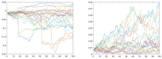
Figure 1. CGMYSV sample paths (left) and CIR sample paths (right).

Table 1. KS test for distributions of simulated sample paths.

	KS Statistic	p-Value
10 days	0.0070	0.7029
25 days	0.0122	0.1026
50 days	0.0069	0.7296
100 days	0.0110	0.1748

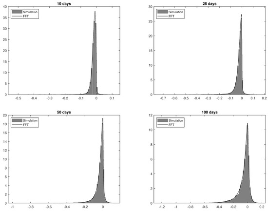
Figure 2. CGMYSV pdfs based on the simulated sample path (gray bar-plots) vs pdf using FFT method (solid curves). Distributions of $X_t$ are for $t=10\Delta t$ (top-left), $t=25\Delta t$(top-right), $t=50\Delta t$ (bottom-left), and $t=100\Delta t$ (bottom-right), where $\Delta t=1/252$ is one day of year fraction.

4. The CGMYSV Option Pricing Model

In this section, we discuss the option pricing model using the CGMYSV model. We define the model and calibrate its parameters using the European style, S&P 500 index option (SPX option) data, and the American style S&P 100 index option (OEX option) data.

Let r and q be the risk-free rate of return and the continuous dividend rate of a given underlying asset, respectively. The risk-neutral price process ${\left\{S_t\right\}}_{t\ge 0}$ of the underlying asset is assumed to be

$$S_t=\frac{S_{0}exp((r-q)t+L_t)}{E\left[exp\left(L_t\right)\right]},$$

(10)

where ${\left\{L_t\right\}}_{t\ge 0}$ is the CGMYSV process with parameters $(\alpha$, ${\lambda }_{+}$, ${\lambda }_{-}$, $\kappa$, $\eta$, $\zeta$, $\rho$, $v_0)$. By (6), we also have

$$S_t=\frac{S_{0}exp((r-q)t+L_t)}{{\Phi }_t(-ilog{\varphi }_{stdCTS}(-i;\alpha ,{\lambda }_{+},{\lambda }_{-}),-\rho i,v_0)}.$$

4.1. Calibration to European Options

For the risk-neutral price process ${\left\{S_t\right\}}_{t\ge 0}$ defined by (10), the European call and put prices, with strike price K and time to maturity T, are given by $C(K,T)=e^{-rT}E\left[{(S_t-K)}^{+}\right]$ and $C(K,T)=e^{-rT}E\left[{(K-S_t)}^{+}\right]$, respectively. Using the fast Fourier transform (FFT) method of Carr and Madan (1999), we can calculate European call/put prices numerically. We calibrate the CGMYSV parameters $(\alpha$, ${\lambda }_{+}$, ${\lambda }_{-}$, $\kappa$, $\eta$, $\zeta$, $\rho$, $v_0)$ using the SPX option prices for 11 September 2017. We observed 247 call prices and 289 put prices on that day. The S&P 500 price, $S_0$, risk-free rate of return, r, and continuous dividend rate, q, on that day were $S_0=2488.11$, $r=1.213\%$, and $q=1.884\%$. The calibration results for SPX calls and puts are provided in Table 2. Figure 3 shows observed SPX call and put prices, and calibrated CGMYSV prices using the FFT.

Table 2. Calibrated Parameters for the SPX option on 11 September 2017.

Parameter	Call	Put
$\alpha$	$0.5184$	$0.0089$
${\lambda }_{+}$	$25.4592$	$2.0852$
${\lambda }_{-}$	$4.6040$	$6.2380$
$\kappa$	$1.0029$	$1.4333$
$\eta$	$0.0711$	$0.1961$
$\zeta$	$0.3443$	$1.1931$
$\rho$	$-2.0283$	$-0.1695$
$v_0$	$0.006381$	$0.0619$

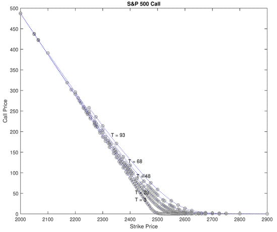
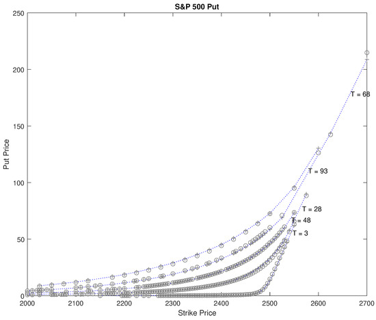
Figure 3. Observed SPX option price and model prices calibrated to the market prices for Call (top) and put (bottom) on September 11, 2017. ‘∘’ stands for the market price and ‘+’ stands for the FFT price.

We recalculate the European call and put prices using the MCS method with the calibrated parameters from Table 2. The sample paths of the MCS method are generated by Algorithm 1. We used 10,000 sample paths. To compare the MCS method with the FFT method, we use the four error estimators: the average absolute error (AAE), the average absolute error as a percentage of the mean price (APE), the average relative percentage error (ARPE), and the root mean square error (RMSE) (see Schoutens (2003)).3 The measured values for these error estimators, for the FFT method and the MCS method, are in Table 3. In all cases but one, for both the call and put cases, the MCS method has larger error values than the FFT method. This is not surprising because we calibrated the parameters using the FFT method. However, while larger, the error values for the MCS method are similar to those of the FFT method. That means the sample path generation with Algorithm 1 performs well, and prices by the MCS perform similarly to those for the FFT method.

Table 3. Error estimators for the parameter calibration to the call and put option market price on 11 September 2017.

	Call			Put
Error	FFT	MCS		FFT	MCS
AAE	$0.4442$	$0.6220$		$0.4047$	$0.5512$
APE	$0.0053$	$0.0074$		$0.0226$	$0.0308$
ARPE	$0.0711$	$0.0813$		$0.2094$	$0.1672$
RMSE	$0.6016$	$0.8019$		$0.7006$	$0.8608$

For the option prices computed with the MCS method, we obtain standard error estimates for each 247 call and 289 put option. (Not presented due to page limitations.) Instead, in Figure 4, we plot MCS prices and the 95% confidence intervals for case $2400<K<2600$, and time to maturity $T=48days$.

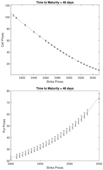
Figure 4. Confidence Intervals for the MCS option prices. Dots are observed market prices, dot-coves are MCS prices, and ‘I’ shape bars are 95% confidence intervals of MCS prices. The first (top) plate is for call option pricing and the second (bottom) plate is for put option pricing.

Finally, we perform the bootstrapping. We select an at-the-money call, and an at-the-money put of $K=2500$ and $T=28days$ as examples, and calculate call and put prices with the MCS parameters in Table 2. Table 4 shows that the MCS prices and their standard errors for 100, 1000, 5000, and 10,000 sample paths. We repeat this process 100 times. Boxplot summaries of the statistics for the resulting call and put prices for each number of sample paths are presented in Figure 5. We also show (by the symbol ’*’) the call/put prices computed using the FFT method. We observe that, as the number of sample paths increases, the interquartile distance of MCS prices narrows to that of the FFT price and dispersions are reduced.

Table 4. MCS prices and standard errors for SPX call and put with the strike price $K=2500$ and time to maturity $T=28days$ using calibrated parameters on 11 September 2017.

	Call			Put
Number of Simulation	Price	Standard Error		Price	Standard Error
100	15.9651	2.1001		34.3371	7.9356
1000	17.8790	0.7511		32.5601	2.2353
5000	19.6536	0.3634		32.7791	1.0458
10,000	19.6840	0.2551		32.6914	0.7617
FFT Price	19.6590			32.9541
Market Price	19.05			31.50

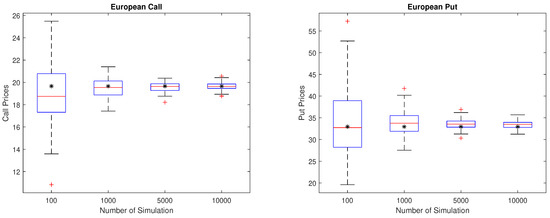
Figure 5. Bootstrapping for call (left) and put (right).

4.2. Calibration to American Options

In Section 4.1, we have seen that the sample path generation method using the series representation works for the MCS method for European option pricing. In this section, we discuss the American option pricing with the same sample path generation method. We use the least squares regression method (LSM) of Longstaff and Schwartz (2001) for American option pricing with the MCS method. When we perform the regression for the expected value of an option, we consider $S_t$, $S_t^2$, ${\sigma }_t$, ${\sigma }_t^2$, and ${\sigma }_t{S}_t$ as independent variables, following the idea in Chapter 15 of Rachev et al. (2011).

For empirical illustration, we use market prices of the American style OEX option. We calibrate the parameters of the CGMYSV model with fixed seed numbers for each random number generation. That is, we fix the seed value for the chi-square random number generator in the CIR process, and generate uniform and exponential random numbers $U_j$, $U_j^{\prime }$, $E_j$, $E_j^{\prime }$, and ${\tau }_j$ with the predefined seed values. Then we set the model parameters, generate $\widehat{CGMYSV}$ sample paths using Algorithm 1 with the fixed seed number and the fixed random number sets, and then calculate American option price using LSM. We find the optimal model parameters to minimize RMSE. As a benchmark, we calibrate the parameters of the CGMY option pricing model (See Carr et al. (2002)) with the OEX option price data using LSM, with sample paths generated by the series representation explained in Section 2.3.

The calibration results are presented in Table 5. We calibrate the CGMY and the CGMYSV model parameters for 12 Wednesdays in 2015 and 2016. Values for the four error estimators, AAE, APE, ARPE, and RMSE, are provided in Table 6. As smaller error values imply better calibration performance, smaller errors are written in bold letters. Table 6 shows that the CGMYSV calibration performs better than the CGMY calibration, except for 10 February 2016, and 10 June 2015. On 9 March 2016, AAE and APE values for the CGMY model are less than those of CGMYSV, but ARPE and RMSE values for CGMY are larger than those for CGMYSV. The ARPE value for CGMY is smaller than that of CGMYSV on 10 November 2015, but the other three error values for CGMY are larger than that for CGMYSV. Therefore, we can conclude that, in this investigation, the CGMYSV option pricing model typically performs better than the CGMY option pricing model, except in a few cases. Hence, the LSM with Algorithm 1 works well for the American option calibration.

Table 5. Parameter Calibration Results for the OEX Option market.

Date	Model	$\mathit{\alpha }$	C	${\mathit{\lambda }}_{+}$	${\mathit{\lambda }}_{-}$	$\mathit{\kappa }$	$\mathit{\eta }$	$\mathit{\zeta }$	${\mathit{v}}_0$	$\mathit{\rho }$
Apr. 6, 2016	CGMY	$0.5459$	$0.3495$	$6.3595$	$7.7563$
	CGMYSV	$1.1356$		$35.2115$	$7.7883$	$1.9322$	$0.3550$	$1.2211$	$0.0100$	$1.2237$
Mar. 9, 2016	CGMY	$1.6885$	$0.0246$	$21.2919$	$2.8805$
	CGMYSV	$0.0353$		$20.3911$	$9.9256$	$2.1262$	$0.4570$	$1.2665$	$0.0236$	$1.3434$
Feb. 10, 2016	CGMY	$0.9287$	$3.5284$	$72.5855$	$46.4594$
	CGMYSV	$0.0257$		$1.3491$	$0.7503$	$2.4301$	$0.4185$	$1.8126$	$0.2711$	$0.3567$
Jan. 6, 20166	CGMY	$1.2290$	$0.4104$	$64.6344$	$21.3096$
	CGMYSV	$1.3081$		$33.2233$	$32.5605$	$2.0656$	$0.4237$	$1.8947$	$0.0810$	$0.1172$
Dec. 9, 2015	CGMY	$1.3241$	$0.2984$	$57.6574$	$30.2749$
	CGMYSV	$0.6308$		$40.5190$	$24.3874$	$5.0247$	$0.3299$	$3.5989$	$0.0593$	$0.2334$
Nov. 10, 2015	CGMY	$1.5907$	$0.0184$	$26.4398$	$2.7714$
	CGMYSV	$0.0266$		$1.6365$	$0.7506$	$1.0354$	$0.5658$	$0.3936$	$0.1111$	$1.2914$
Oct. 7, 2015	CGMY	$0.9792$	$0.2955$	$53.8624$	$8.4758$
	CGMYSV	$0.8763$		$65.0630$	$67.4571$	$1.8555$	$0.2794$	$2.1050$	$0.0422$	$0.0080$
Sep. 9, 2015	CGMY	$1.2572$	$0.5862$	$54.0807$	$15.3905$
	CGMYSV	$0.5836$		$30.2731$	$17.2115$	$5.1193$	$0.3569$	$4.8231$	$0.1189$	$0.1158$
Aug. 12, 2015	CGMY	$0.7574$	$0.5926$	$61.7876$	$14.2761$
	CGMYSV	$0.4848$		$42.9235$	$31.7027$	$2.1644$	$0.1964$	$2.1032$	$0.0283$	$0.1639$
Jul. 8, 2015	CGMY	$1.1742$	$0.2429$	$78.6224$	$11.4198$
	CGMYSV	$0.9127$		$46.3671$	$46.3013$	$2.2125$	$0.2173$	$2.0394$	$0.0547$	$-0.0637$
Jun. 10, 2015	CGMY	$1.3849$	$0.0407$	$64.9276$	$7.8355$
	CGMYSV	$0.0391$		$1.0381$	$0.7820$	$1.1451$	$0.6167$	$0.6062$	$0.0518$	$1.2736$
May. 6, 2015	CGMY	$1.2247$	$0.1125$	$87.0744$	$8.6069$
	CGMYSV	$0.8628$		$53.8182$	$54.3726$	$2.0949$	$0.2023$	$2.0731$	$0.0352$	$0.0647$

Table 6. Error Estimates for the calibration of the OEX option.

Date	Model	AAE	APE	ARPE	RMSE
Apr. 6, 2016	CGMY	0.6623	0.1726	0.4587	0.8833
	CGMYSV	0.1881	0.0490	0.1242	0.2497
Mar. 9, 2016	CGMY	0.6780	0.1106	0.2871	0.8323
	CGMYSV	0.6833	0.1115	0.2492	0.8086
Feb. 10, 2016	CGMY	0.7755	0.0513	0.1282	1.1076
	CGMYSV	0.9267	0.0613	0.2075	1.2042
Jan. 6, 2016	CGMY	0.6945	0.0644	0.1617	0.9379
	CGMYSV	0.4140	0.0384	0.0784	0.6574
Dec. 9, 2015	CGMY	0.7986	0.0931	0.1855	1.1230
	CGMYSV	0.5903	0.0688	0.0957	0.7885
Nov. 10, 2015	CGMY	0.3137	0.0576	0.2169	0.4159
	CGMYSV	0.2337	0.0429	0.2560	0.3815
Oct. 7, 2015	CGMY	0.5268	0.1018	0.3741	0.6891
	CGMYSV	0.2186	0.0423	0.1520	0.3221
Sep. 9, 2015	CGMY	0.8948	0.0880	0.1681	1.2499
	CGMYSV	0.5874	0.0577	0.1002	0.9153
Aug. 12, 2015	CGMY	0.6464	0.0941	0.1894	0.9097
	CGMYSV	0.4137	0.0602	0.1401	0.5652
Jul. 8, 2015	CGMY	0.7636	0.0800	0.1456	1.0079
	CGMYSV	0.2518	0.0264	0.1023	0.3238
Jun. 10, 2015	CGMY	0.2535	0.0671	0.2576	0.3483
	CGMYSV	0.3180	0.0841	0.3676	0.4120
May. 6, 2015	CGMY	0.7361	0.0765	0.1479	0.9776
	CGMYSV	0.3880	0.0403	0.1097	0.5137

Finally, we perform bootstrapping. We selected the at-the-money, 6 April 2016 put option with strike price $K=910$ and $T=31$ days to maturity. Put prices were obtained by LSM using the parameters calibrated for that day in Table 5. On that day, the underlying S&P 100 index price was 918.21, and the market put price was 13.95. Table 7 shows the LSM prices and their standard errors for simulation using 100, 1000, 5000, and 10,000 sample paths. The LSM prices approach the market price, and the standard error decreases as the number of sample paths increases. We repeated these simulations 100 times, and present numerical summaries for the statistics for those 100 prices in Table 8. As the number of sample paths increases, means and medians approach the market put price, while the standard deviations and ranges are decreased. We present boxplot summaries in Figure 6 for those 100 prices. Market put prices are also represented (’*’ symbols) with the boxplots. We observe that the interquartile distance of LSM prices narrows to that of the market price, and dispersions are reduced as the number of sample paths increase.

Table 7. MCS prices and standard errors for the OEX put with time to maturity of $T=31days$ and strike price $K=910$ using parameters calibrated on 6 April 2016.

	Put
Number of Simulation	Price	Standard Error
100	15.4565	2.7280
1000	15.0373	1.0173
5000	13.9616	0.3990
10,000	13.8768	0.2856
Market Price	13.950

Table 8. Numerical Summary of the bootstrapping. We repeat the MCS pricing 100 times for various number of simulation, and calculate basic statistics for the 100 MCS put prices.

Number of
Simulation	Mean	Std	Q1	Median (Q2)	Q3	IQR	Range
100	16.6119	3.2399	14.3966	16.5589	18.6850	4.2885	21.9747
1000	14.4190	0.7568	13.9394	14.4343	14.8609	0.9215	3.9857
5000	14.0073	0.3258	13.8295	14.0252	14.1876	0.3581	1.8799
10,000	13.8599	0.2524	13.6766	13.8640	14.0410	0.3644	1.1730
Market Price	13.950

Std: Standard Deviation, Q1: the 1st quartile, Q2: the 2nd quartile, Q3: the 3rd quartile, IQR: inter quartile range.

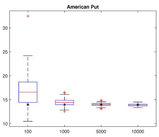
Figure 6. Bootstrapping for OEX put option with time to maturity of $T=31days$ and strike price $K=910$.

Figure 7 provides a graphical illustration of the calibration for 6 April 2016. Calibrated CGMYSV prices are drawn by "×", the market observed prices are drawn by "∘", and the 95% confidence intervals are marked by a "I" shape. The days to maturities T are written on the plate.

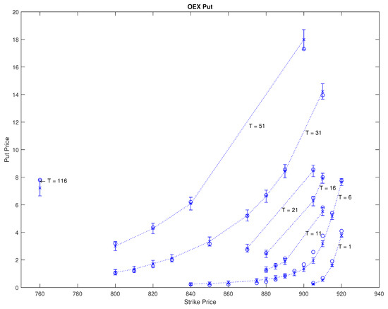
Figure 7. OEX put prices on April 6, 2016 and LSM prices with their confidence intervals. Circles (‘∘’) are observed OEX put prices, ‘×’ points are LMS prices, and ‘I’ shape bars are 95% confidence intervals of LMS prices.

4.3. Asian and Barrier Options

The sample path generation method for the CGMYSV model can also be used for Asian and Barrier option pricing. In this section, we briefly show examples of Asian and Barrier option pricing using the MCS, with sample paths generated by Algorithm 1. We generated 10,000 sample paths of the CGMYSV model with parameters $\alpha =0.52$, ${\lambda }_{+}=25.46$, ${\lambda }_{-}=4.604$, $\kappa =1.003$, $\eta =0.0711$, $\zeta =0.3443$, $v_0=0.0064$, and $\rho =-2.0280$. Then, we generated the underlying price process ${\left\{S_t\right\}}_{t\ge 0}$ using (10), where $S_0=2,488$, $r=0.0121$, and $d=0.0188$.

For the Asian option, we consider the arithmetic average call and put prices for strike price $K=2500$ and a time to maturity of $T=25days$. Table 9 shows the MCS prices for Asian call & put prices and their standard errors for simulations with 100, 1000, 5000, and 10,000 sample paths. The standard error of the MCS prices decreased as the number of sample paths increased. We repeated this process 100 times, and present boxplots for those 100 prices in Figure 8. We observe that the MCS prices converge, and dispersions are reduced as the number of sample paths increase.

Table 9. MCS prices and standard errors for Asian call & put.

	Call			Put
Number of Simulation	Price	Standard Error		Price	Standard Error
100	22.0834	1.7485		11.7400	3.4463
1000	21.0078	0.5866		9.7009	1.0759
5000	21.4664	0.2785		10.5634	0.5443
10,000	21.6513	0.1937		9.9964	0.3679

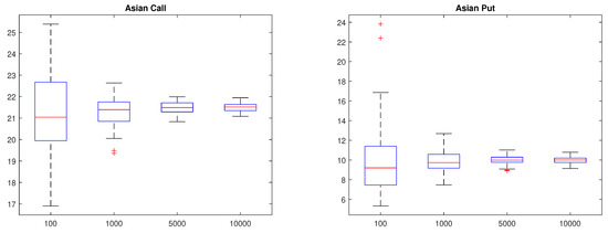
Figure 8. Bootstrapping for Asian call (left) & put (right).

Similarly, we found the MCS price for Barrier options. We considered the down-and-out call and the up-and-out put Barrier options having a strike price of $K=2500$ and time to maturity of $T=25days$. Barriers of the down-and-out call and the up-and-out put are 2400, and 2750, respectively. Table 10 shows the MCS prices and their standard errors for simulations with 100, 1000, 5000, and 10,000 sample paths. The standard error of the MCS prices decreased as the number of sample paths increased. We repeated this process 100 times, and present boxplots for those 100 prices in Figure 9. We also observe that the MCS prices converged, and dispersions are reduced as the sample paths increase.

Table 10. MCS prices and standard errors for the down-and-out call and the up-and-out put.

	Down & Out Call			Up & Out Put
Number of Simulation	Price	Standard Error		Price	Standard Error
100	12.9019	1.4535		36.2543	3.6254
1000	15.3738	0.5165		30.0687	0.9509
5000	16.6097	0.2460		31.8030	0.4498
10,000	16.5518	0.1749		30.2590	0.3026

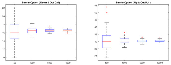
Figure 9. Bootstrapping for Barrier options: the down-and-out call (left) and the up-and-out put (right).

5. Conclusions

In this paper, we developed the CGMYSV sample path generation algorithm using the discrete-time approximation method with series representation. Performance of the discrete-time approximation of the CGMYSV process was tested by comparing the simulated distribution to the pdf calculated by the inverse Fourier transform method. We applied the sample path generation algorithm to European and American option pricing with MCS and LSM. We compared the MCS method to the FFT method in European option pricing with the SPX option market data. We calibrated the parameters of the CGMYSV model to the American style OEX option using LSM. We measured the performance of the calibration using four error estimators and the boot-strapping method. We conclude that the sample path generation method of the CGMYSV model performs well, and can successfully be applied to American option pricing with LSM. Finally, we also presented Asian and Barrier option pricing examples with the MCS method using the sample path generation algorithm.

References

- Bianchi, Michele Leonardo, Svetlozar T. Rachev, Young Shin Kim, and Frank J. Fabozzi. 2010. Tempered infinitely divisible distributions and processes. Theory of Probability and Its Applications (TVP), Society for Industrial and Applied Mathematics (SIAM) 55: 58–86. [Google Scholar] [CrossRef]
- Black, Fischer, and Myron Scholes. 1973. The pricing of options and corporate liabilities. The Journal of Political Economy 81: 637–54. [Google Scholar] [CrossRef]
- Boyarchenko, Svetlana I., and Sergei Z. Levendorskiĭ. 2000. Option pricing for truncated Lévy processes. International Journal of Theoretical and Applied Finance 3: 549–52. [Google Scholar] [CrossRef]
- Carr, Peter, Hélyette Geman, Dilip B. Madan, and Marc Yor. 2002. The fine structure of asset returns: An empirical investigation. Journal of Business 75: 305–32. [Google Scholar] [CrossRef]
- Carr, Peter, Hélyette Geman, Dilip B. Madan, and Marc Yor. 2003. Stochastic volatility for Lévy processes. Mathematical Finance 13: 345–82. [Google Scholar] [CrossRef]
- Carr, Peter, and Dilip Madan. 1999. Option valuation using the fast fourier transform. Journal of Computational Finance 2: 61–73. [Google Scholar] [CrossRef]
- Cox, John C., Jonathan E. Ingersoll, Jr., and Stephen A. Ross. 1985. A theory of the term structure of interest rates. Econometrica 53: 385–407. [Google Scholar] [CrossRef]
- Heston, Steven L. 1993. A closed-form solution for options with stochastic volatility with applications to bond and currency options. Review of Financial Studies 6: 327–43. [Google Scholar] [CrossRef]
- Hurst, Simon R., Eckhard Platen, and Svetlozar Todorov Rachev. 1999. Option pricing for a logstable asset price model. Mathematical and Computer Modeling 29: 105–19. [Google Scholar] [CrossRef]
- Kim, Young Shin, Svetlozar T. Rachev, Michele Leonardo Bianchi, Ivan Mitov, and Frank J. Fabozzi. 2011. Time series analysis for financial market meltdowns. Journal of Banking and Finance 35: 1879–91. [Google Scholar]
- Kim, Young Shin, Svetlozar T. Rachev, Michele Leonardo Bianchi, and Frank J. Fabozzi. 2010. Tempered stable and tempered infinitely divisible GARCH models. Journal of Banking and Finance 34: 2096–109. [Google Scholar] [CrossRef]
- Koponen, Ismo. 1995. Analytic approach to the problem of convergence of truncated Lévy flights towards the gaussian stochastic process. Physical Review E 52: 1197–99. [Google Scholar] [CrossRef] [PubMed]
- Lamberton, D., and B. Lapeyre. 1996. Introduction to Stochastic Calculus Applied Finaice. London: Chapman & Hall/CRC. [Google Scholar]
- Longstaff, Francis A., and Eduardo S. Schwartz. 2001. Valuing American options by simulation: A simple least-squares approach. Review of Financial Studies 14: 113–48. [Google Scholar] [CrossRef]
- Rachev, Svetlozar T., Young Shin Kim, Michele Leonardo Bianchi, and Frank J. Fabozzi. 2011. Financial Models with Lévy Processes and Volatility Clustering. New York: John Wiley & Sons. [Google Scholar]
- Mittnik, Stefan, Svetlozar T. Rachev, and Marc S. Paolella. 2000. Stable Paretian Models in Finance. New York: John Wiley & Sons. [Google Scholar]
- Rosiński, Jan. 2007. Tempering stable processes. Stochastic Processes and Their Applications 117: 677–707. [Google Scholar] [CrossRef]
- Schoutens, Wim. 2003. Lévy Processes in Finance: Pricing Financial Derivatives. Chichester: John Wiley and Sons. [Google Scholar]