Article

Subjective Return Expectations, Perceptions, and Portfolio Choice †

1
Economics and CPC, Highfield Campus, University of Southampton, Bld 58, R3113, ESPS, FSS, Southampton SO171BJ, UK
2
ILB, 75002 Paris, France
3
CFS, University of Wisconsin-Madison, Madison, WI 53706, USA
4
Applied Economics, Universitat de les Illes Balears, 07122 Palma de Mallorca, Spain
5
PSE-CNRS, 75014 Paris, France
*
Author to whom correspondence should be addressed.
The authors thank Toke Aidt, Alberto Bisin, Charles Bellemare, Antonio Cabrales, Chris Carroll, Tiago Cavalcanti, Giancarlo Corsetti, Adeline Delavande, Richard Disney, George Evans, Pam Giustinelli, Michael Haliassos, Mike Hurd, Gabor Kézdi, John Knowles, Christos Koulovatianos, Hamish Low, Chuck Manski, Andre Masson, Nicola Pavoni, Victor Rios-Rull, Mark Salmon, Kjetil Storesletten, Jian Tong, Giorgio Topa, Bob Willis, and Basir Zafat for their various comments and suggestions, and seminar audiences at the NBER 2012 Summer Institute Economic Fluctuations and Growth working group on “Aggregate Implications of Microeconomic Consumption Behaviour”, at the 2012 CIRPEE workshop on “Formation and revision of subjective expectations” in Quebec City, at the 2013 NHH-UiO workshop on economic dynamics, the 2014 Barcelona GSE Learning in Macroeconomics and Finance workshop, Goethe University Frankfurt, Nottingham University, Universite de Paris-Dauphine, Universitat de les Illes Balears, Univeristy of Salerno and at the University of Cambridge. The last author gratefully acknowledges financial support from the “Agence Nationale pour la Recherche” (ANR), and the first from the ESRC (RES-061-25-0327), as well as hospitality by the University of Cambridge and the Universitat de les Illes Balears.
J. Risk Financial Manag. 2022, 15(1), 6; https://doi.org/10.3390/jrfm15010006
Submission received: 2 November 2021 / Revised: 5 December 2021 / Accepted: 7 December 2021 / Published: 30 December 2021
(This article belongs to the Special Issue Household Finance)

Abstract

:
Exploiting a representative sample of the French population by age, wealth, and asset classes, we document novel facts about their expectations and perceptions of stock market returns. Both expectations and perceptions of returns are very dispersed, significantly lower than their data counterparts, and a substantial portion of the variation in the former is explained by dispersion in the latter. Consistent with portfolio choice models under incomplete information, a conditional risk-return trade-off explains the intensive margin, while at the extensive margin, only expected returns matter. Despite accounting for survey measurement error in subjective return expectations, ’muted sensitivities’ at both portfolio choice margins obtain, getting consistently (i) bigger when excluding informed non-participants, and (ii) smaller, for inertial and professionally delegated portfolios.
JEL Classification:
D12; D83; D84; G11; C42

1. Introduction

Since the advent of the 2008 financial crisis, household finances have been under the spotlight, both in the media and in academia—and rightly so: households are the end owners of property, financial, and business assets in the economy, holding about three times more assets than firms and about the same liabilities in the aggregate, see Tufano (2009).1 Although institutions collectively manage 68% of those assets in the US, 32% are directly managed by households, with the former explaining about 45% of the cross-sectional variance of stock returns and the latter 47% (see Koijen and Yogo 2019). The key issue is therefore whether households manage those assets ’rationally’, i.e., according to the principles of economic theory (e.g., Campbell 2006, 2016).
The field of household/consumer finance has identified systematic deviations of observed financial behaviour from the positive predictions of workhorse models in finance (see Guiso and Sodini 2013 or Gomes et al. 2021 for comprehensive recent surveys). Central to any portfolio allocation model is that, to invest in stocks, a person needs to make a trade-off between the returns and risks expected in the stock market: Haliassos and Bertaut (1995) find that a majority of households do not invest in stocks despite of the historically positive equity premium (see Dimson et al. 2012), or ’stock market non-participation puzzle’. Conditional on participating, Ameriks et al. (2020) provide evidence of a substantial ’attenuation puzzle’ at the intensive margin, i.e., they find a ’muted response’ of stockholders’ portfolios to expectations and preferences, even after accounting for survey measurement error.2 Although the literature disagrees on the exact shape of the utility function or other factors involved in the decision-making to date (e.g., labour income, business risk or the relevant investment horizon), information and transaction costs remain the most important frictions quantitatively (e.g., Vissing-Jorgensen 2002; Haliassos and Michaelides 2003 or Fagereng et al. 2017).
In this paper, we examine how much of the basic risk-return trade-off the average person understands, and how does it relate to the person’s investment decisions given what she knows. We report empirical results from a representative survey of households in France by wealth, age, and asset classes, containing detailed information on their beliefs about both expected and realised stock market returns, to examine their role in household portfolios at both margins. How aware households are about recently realised stock market returns at the time of the survey allows us to characterize the extent to which households are cognizant of the recent stock market index performance, the extent to which it affects households’ expectations about future returns, and thereby, their portfolios.
Just as we do here, some recent empirical contributions rely on novel survey question formats that enable researchers to elicit quantitatively individual beliefs and the uncertainty surrounding them, Manski (2004), both about the future (forecasts) and the recent past (now/backcasts). Given that information about realised stock market index returns over different horizons is public and readily available, household beliefs about them are informative of how ignorant households are and the extent to which expectations about returns rely on them. Evidence in support of misperceptions about facts driving beliefs about the future has been found for professional forecasters’, Andrade and Le Bihan (2013), firms’, Coibion et al. (2018), and consumers’ (Jonung and Laidler 1988; Armantier et al. 2016; Armona et al. 2019) beliefs about inflation, as postulated by models of imperfect information (e.g., Woodford 2013) or of rational inattention (Sims 2003; Reis 2006; Alvarez et al. 2012; Abel et al. 2007 or Abel et al. 2013). Recent empirical evidence on ’stock return ignorance’ driving US household decisions to invest in stocks has been advanced by Merkoulova and Veld (2021). The crucial role of heterogeneous subjective beliefs for disciplining heterogeneous agent models and understanding the macroeconomy has been advocated, among others, by Carroll (2017) or Manski (2018).
After assessing the high quality of our data, we document a number of new stylised facts about the stock market beliefs that households hold. Households’ average forecasts about returns are significantly lower and less volatile than their counterparts computed from long-run historical data (e.g., Le Bris and Hautcoeur 2010 or Dimson et al. 2012). Similarly, household perceptions about realised returns are on average 41% lower than the actual returns, and are reported with considerable noise, denoting ignorance/unawareness. Importantly, and in line with what happens with inflation (e.g., Coibion et al. 2018), there is substantial cross-sectional disagreement in beliefs, being larger about facts (realised returns) than about future events (future or expected returns). Furthermore, expectations and perceptions are strongly correlated, suggesting that ignorance about recent stock market performance is an important novel factor in accounting for heterogeneity in expected returns: around 15% of the puzzling heterogeneity in respondents’ stock market return expectations previously identified in the literature by Dominitz and Manski (2007) (see also Kézdi and Willis 2009, or Hurd et al. 2011) is explained by differences in subjective perceptions of returns. Turning to what are the sources of variation in ignorance across households, we find evidence that the affluent, males, and those who bank online, or have parents who own stocks, are more aware, and display more confidence about facts than females, those less well-off, earning less, with no access to online banking or stockholding parents.
Relative to the aforementioned works, we estimate a sample selection model that allows to separately identify the effect of conditional subjective expectations at both the extensive and intensive margins on households’ demand for risky assets. To account for survey measurement error (as in Ameriks et al. 2020) and for the incomplete information upon which respondents estimate future returns (e.g., Klein and Bawa 1976 or Gennotte 1986), we deploy a control function approach that controls for errors in estimating expected returns on household portfolios. Conditioning on perceptions of returns as a measure of how knowledgeable households are, we find that (i) mean subjective stock market return expectations determine both margins, but that (ii) the subjective standard deviation of returns only determines conditional asset shares, in line with canonical models of portfolio choice. (iii) The estimated effects are quantitatively important: conditional on demographics, endowments, constraints, measures of time and risk preferences, trust, as well as on various measures of inertia and delegation in portfolio management, a one percentage point (pp) increase in the average expectation of returns (from its sample 5-year average of 5.9% to 6.9%) increases the probability of stock ownership by 0.7 percentage points (corresponding to a 2.59% increase relative to the unconditional likelihood of 27%), and the share of wealth invested in risky financial assets by 3.2 percentage points (corresponding to a 7.1% increase, relative to the unconditional mean share of 45%). A one percentage point increase in the subjective standard deviation reduces the conditional asset shares by 2.8 percentage points, representing a 5.7% relative drop. The findings appear robust in population subgroups by gender, age, and total wealth, with portfolio shares of those below median wealth mostly determined by stock market risk while those of the relatively better-off mostly driven by expected returns at both margins. Performing several counterfactual placebo tests, we consistently find that inertial respondents (who have not traded in the stock market over the previous year) and respondents who have fully or partially delegated their portfolio choices to a professional manager, make stockholding decisions that are insensitive to their beliefs about future returns, and hence, to how much do they know. Finally, excluding those who, albeit informed, do not hold stocks for liquidity reasons, magnifies the effect of conditional expectations on households’ portfolios. Hence, household portfolio choices appear consistent with prescriptions of workhorse models of portfolio choice, albeit quantitatively, they fall short of their theoretical benchmarks, in line with Ameriks et al. (2020) ’attenuation puzzle’.3
Related Literature
The recent literature on financial literacy has documented the prevalence in the population of puzzling gaps in elementary financial notions (e.g., Lusardi and Mitchell 2014), or in financial competence (e.g., Ambuehl et al. 2021), in the presence of which optimal financial decisions appear beyond reach, and resulting in substantial differences in wealth accumulation patterns when compounded through the individual life cycle (e.g., Lusardi et al. 2017). Lusardi and Mitchell (2014) define financial literacy by ‘…peoples’ ability to process economic information and make informed decisions about financial planning, wealth accumulation, debt, and pensions’.4 Instead, how aware households are about the most recent realisation of cumulative stock market index returns, measured by their subjective elicited beliefs or perceptions, refers to the ’stock of knowledge’ rather than to the ’ability to exploit that knowledge’. As such, it also differs from ’cognitive ability’.5
Incipient research in survey expectations, building upon Manski (2004) and reviewed in Hurd (2009), uncovers that household expectations regarding the future evolution of the stock market are: (a) for the majority, no better than a 50–50 chance that the stock market index will go up in the year ahead, and extremely heterogeneous (see Dominitz and Manski 2007 and Dominitz and Manski 2011); (b) able to explain differences in financial choices both at a point in time and through the life cycle (e.g., Dominitz and Manski 2007, Miniaci and Pastorello 2010 or Hurd et al. 2011); and (c) able to identify households’ implicit risk preferences, when combined with data on financial choices (e.g., Kézdi and Willis 2009)6. An important assumption in that literature is that, since the stock market is a public non-manipulable event, perfect/common information across respondents is implicitly assumed, at odds with the findings reported here (and elsewhere, e.g., Jonung and Laidler 1988).
Do households’ form return expectations on the basis of what they know? Much of the aforementioned literature implicitly or explicitly assumes so. Here, we examine whether households form expectations about future returns on the basis of what they report to know, as implied by models of imperfect/incomplete information (e.g., Klein and Bawa 1976; Gennotte 1986; Duffie and Sun 1990; Sims 2003; Abel et al. 2007; Abel et al. 2013 or Alvarez et al. 2012). And in line with recent findings reported by Armantier et al. (2016) or by Coibion et al. (2018) for consumer and firm CE/FO perceptions about inflation, respectively,7 We find that the average household’s beliefs about future returns are mostly determined by their perception about realized returns.
To gain further insight into how do agents make financial decisions, renewed research effort has been undertaken theoretically (e.g., Pástor and Veronesi 2009, or Van Nieuwerburgh and Veldkamp 2010; reviewed in Brandt 2010), empirically (e.g., Fagereng et al. 2017) and more recently, experimentally (e.g., Kuhnen 2015), both within and across countries (e.g., Badarinza et al. 2016). Empirically, survey data have been exploited for (i) professional forecasters (e.g., Malmendier and Nagel 2011, Malmendier and Nagel 2016; Amromin and Sharpe 2013; Bordalo et al. 2018); (ii) stock market investors (e.g., Vissing-Jorgensen 2004), for (iii) specific population subgroups, including non-stockholders (by age, Dominitz and Manski 2007, Dominitz and Manski 2011; Kézdi and Willis 2009); for (iv) brokerage account holders (e.g., Ameriks et al. 2020; Giglio et al. 2021); or for (v) a representative sample of the population by age and wealth (e.g., Hurd et al. 2011, Miniaci and Pastorello 2010 or Merkoulova and Veld 2021). Here, we exploit unique data from a new wave of the Taylor Nelson Sofres French survey (TNS 2007), which contains information on attitudes, preferences, subjective expectations, perceptions, and socioeconomic and demographic characteristics for a representative sample of 3826 households, by age, wealth, and asset classes (Campbell 2006).
The rest of the paper is organized as follows: in Section 2, we describe the methodology used to elicit perceptions and expectations of returns, and describe sample measures from in the TNS 2007 survey wave as well as the data set. Section 3 presents the econometric specification and reports the main estimation results of the risky asset demands of households. Finally, in Section 4, we conclude.

2. Measuring Expectations and Perceptions

2.1. Survey Design

In surveys, respondents were asked to state their perceptions of a future event in order to understand if it determined their current behaviour. The recent literature on measuring expectations privileges the use of probability questions rather than eliciting point expectations or the traditional qualitative approach of attitudinal research (see Manski 2004 and Manski 2018). Answers to such questions are used to understand if expectations and outcomes are related, and to evaluate if individual behaviour changes in response to changes in expectations. Dominitz and Manski (2007) elicited the individuals’ expectations of stock market returns inquiring about how ‘well’ the respondents thought a broad-based stock market index, such as the US Standard & Poor’s 500, would do in the year ahead. They exploited data for a representative sample of the elderly from the 2004 wave of the U.S. Health and Retirement Study (HRS).
We build upon their work, and extend their methodology along different dimensions. First, by extending the forecasting horizon to five years, we intend to untie expectational answers from the business cycle conditions prevailing at the time of the survey (March 2007) to better capture (i) the historic average upward trend of the stock market index, and (ii) inertia in portfolio management (e.g., Bilias et al. 2010). The latter is important since it remains an open question with which horizon households invest in the stock market. Second, following the methodology of Guiso et al. (1996) in the Survey on Household Income and Wealth (SHIW) conducted by the Bank of Italy, probability densities are elicited on seven points of the outcome space, instead of just two points of the cumulative distribution functions (cdfs.), to obtain more precise individual estimates of the relevant moments. Third, we exploit data from a sample representative of the population by age, wealth, and asset classes, to examine the relationship between the demand for stocks and subjective expectations at both the intensive and extensive margins (see Campbell 2006 and Campbell 2016). Finally, and most relevant, probabilistic elicitation of the realised cumulative stock market return over the five years immediately prior to fielding the survey, provides a quantitative measure of households’ stock of knowledge, which is domain-specific, retrospective (i.e., publicly available) and relevant in informing subjective expectations of returns (e.g., Gennotte 1986, Coibion et al. 2018 or Armona et al. 2019). Without it, households that do not invest because they expect the stock market to burst over the given forecasting horizon are indistinguishable from those that do not invest because they are unaware of the investment opportunities offered by the stock market.

The Data

The 2007 wave of the Taylor Nelson Sofres French survey (TNS 2007) was designed by researchers at the Paris School of Economics (PSE), and administered by Taylor Nelson Sofres, a professional agency paid with research funds from the Agence Nationale de la Recherche (ANR). The first wave, carried in 2002, had no questions related to stock market expectations. The 2007 wave contained very detailed information on attitudes, preferences, and expectations, in addition to wealth, income, and socioeconomic and demographic characteristics for a representative sample of French households. A questionnaire was sent to a representative sample of 4000 individuals, corresponding to an equivalent number of households. Respondents had to fill out the questionnaire, and return it by the post in exchange of around EUR 25 in coupon tickets (bons-d’achat).8 3826 respondents sent their questionnaires back, representing a 97% response rate. Within these 3826 respondents, we identified 2039 in which the respondent gave complete answers to questions on beliefs about returns and stock holdings, representing a 53% response rate.
The overall and estimation sample descriptive statistics for the main variables and covariates are reported in Table 1. Only 27% of respondents hold stocks directly or indirectly, investing around 45% of their financial wealth in stocks in our estimation sample. Although stockholding status is in line with results reported for other European countries (e.g., Badarinza et al. 2016), the conditional shares are slightly above the 30% average reported for France in Guiso et al. (2002) (better corresponding to the overall sample mean). In addition, households in the estimation sample are more risk averse (as measured by their coefficient of constant absolute risk aversion, CARA), slightly less impatient (Temporal preference), are more likely to live in Paris, younger, are less often females, and are better educated than in the overall sample. They are also more likely to be high income earners and to be wealthier, and display more optimistic beliefs about future returns (ER), albeit perceiving a higher associated risk, as measured by the standard deviation of expected returns (Sd ER). Finally, households in our estimation sample appear more aware about realized returns (PR) albeit less confident (Sd PR): the last two columns of Table 1 compare estimation sample statistics for respondents (’NR(PR) = 0’) versus non-respondents (’NR(PR) = 1’) to the perception questions about realised cumulative returns: the latter appear less likely to be stockholders and invest lower shares of their financial wealth in stocks conditional on participating, in line with results reported by Merkoulova and Veld (2021) for US households.
The survey was conducted in March 2007. Figure 1 shows that, after a drop of nearly 60% in the French stock market Index (CAC-40)9, caused by the ’dot-com crash’ of 2001, by the time the survey was conducted (vertical green bar), the stock market index had been steadily recovering since the mid 2002. In March 2007, the index was still below its ’dot-com’ peak. Because the CAC-40 is regularly covered by both specialised and general news media, it is likely that respondents were particularly aware of the recent stock market evolution, and provide very heterogeneous and uncertain answers regarding the stock market prospects for the five years to come, given the recent experience of a bust and a boom.
Since the survey was conducted in March 2007, exploiting available public information from historical monthly data between July 1987 and July 2011 produces relevant sample first and second moments ( μ = 0.023 ) μ ( 5 ) = 0.108 and ( σ = 0.10 ) σ ( 5 ) = 0.19 of nominal (yearly, and) 5-year cumulative log returns on the CAC-40. Besides being broadly consistent with moments computed from long historical series—reported in Dimson et al. (2012) and, corrected for survivorship bias, in Le Bris and Hautcoeur (2010), for France 1900–2005, and 1854–2007, respectively—those sample moments characterise the subjective beliefs of those respondents who would base them on the history of observed stock market index closing values at a monthly frequency.10

2.2. Expectations

To measure expectations, we elicited households’ subjective beliefs regarding the likely evolution of the stock market index five years ahead in time, I t + 5 , relative to March 2007, I t , from the following questions (translated wording):
c6. ’Five years from now, do you think that the stock market…For each category write down the likelihood of occurrence assigning a value between 0 and 100. The sum of all your answers must be equal to 100:
  • …will have increased by more than 25%;
  • …will have increased by 10 to 25%;
  • …will have increased by less than 10%;
  • …will be the same;
  • …will have decreased by less than 10%;
  • …will have decreased by 10 to 25%;
  • …will have decreased by more than 25%.
c7b. ’In your opinion, if you expect the stock market to increase within the next 5 years, which would be the highest possible increase (as a percentage)?’
c8b. ’In your opinion, if you expect the stock market to decrease within the next 5 years, which would be the lowest possible decrease (as a percentage)?’
Question c6 (qc6) inquires household i about the subjective relative likelihood of occurrence, p t + 1 , k i , of each of the seven alternative scenarios, k = 1 , , 7 . Each scenario represents a possible outcome range for the percentage change in the index between t and t + 5 , R t + 1 ( 5 ) I t + 5 I t 1 .11 Questions c7b and c8b provide subjective upper and lower bounds for the percentage change, R max i and R min i , respectively12, e.g., R min i captures the ’maximum drawdown (MDD)’, a risk-metric statistic commonly used by professional investors to gauge the likelihood of worst case cumulative return scenarios over a given time window. The corresponding outcome ranges are:
R t + 1 [ R min i , 0.25 ) k = 1 , [ 0.25 , 0.10 ] , k = 2 ( 0.10 , 0 ) , k = 3 { 0 } , k = 4 ( 0 , 0.10 ) , k = 5 [ 0.10 , 0.25 ] k = 6 , ( 0.25 , R max i ] k = 7
and households’ subjective likelihoods are accordingly:
p t + 1 , k i Pr i R t + 1 k = Pr i I t + 5 I t 1 k , i
and zero elsewhere, i.e., R t + 1 ( , R min i ) ( R max i , + ) .
Table 2 reports the distribution of survey responses to expectations (and perceptions) of cumulative stock market returns questions, imposing a uniform distribution within the different outcome ranges. Out of the 3826 overall sample respondents, around 63% (2406) meaningfully answered the expectations question. Moreover, 328 cases were excluded as the sum of their answers did not round up to 100.13 Figure 2 below depicts the histogram, which averages the individual probability density functions of those who answered, with almost 40% of respondents expecting a stock market cumulative return of zero between March 2007 and March 2012 (modal response). Table 2 (upper panel) reports the quartiles of the distribution. The reported survey mean and standard deviation of returns are about one half and one third, respectively, of the first and second moments computed by Dimson et al. (2012), or Le Bris and Hautcoeur (2010) exploiting the long-run history of realisations.14
This finding is confirmed in our estimation sample, where all 2039 respondents provided a valid response to the expectations question (Table 2, lower panel). By March 2007, household beliefs about cumulative stock market returns underestimated, by at least one half, the mean (ER, μ i t + 1 ) and the risk (Sd ER, σ i t + 1 ) relative to moments based on the historical record.15

2.3. Measuring Perceptions

How aware were households about the historical record when forming those beliefs about future returns? The literature on portfolio choice problems (e.g., Brandt 2010 or Biais et al. 2010) has long acknowledged that ’when selecting optimal portfolios, investors have to take into account the fact that ”true” portfolio returns’ can only be estimated with error using the observable instantaneous realized returns on investment’ (Gennotte 1986, p. 733). We therefore inquired respondents about the most recent cumulative stock market return, deploying a similar probabilistic elicitation format to capture: (i) how confident respondents are when conveying their answers about facts16, in addition to (ii) how knowledgeable (or ignorant) they are as well as (iii) the relationship between expectations and perceptions about returns.17
The TNS 2007 survey wave inquires respondents about the likely evolution of the stock market index over the past five years, I t 5 , relative to the time of the interview (March 2007), I t , as follows (translated wording):
c9. ’Over the past five years, do you think that the stock market…For each category write down the likelihood of occurrence assigning a value between 0 and 100. The sum of all your answers must be equal to 100:
  • …has increased by more than 25%;
  • …has increased by 10 to 25%;
  • …has increased by less than 10%;
  • …has remained the same;
  • …has decreased by less than 10%;
  • …has decreased by 10 to 25%;
  • …has decreased by more than 25%.
Question c9 (qc9) inquires household i about the subjective relative likelihood of occurrence, p t , k i , of each of the seven alternative scenarios, k = 1 , , 7 . Each scenario represents a possible outcome range for the percentage change in the index between t 5 and t, R t ( 5 ) I t I t 5 1 . Since ranges k = 1 and k = 7 are unbounded, we set ( R max , R min ) to match observed values.The outcome ranges for R t are therefore identical to those of question c6 described above. Accordingly, households’ subjective likelihoods are given by:
p t , k i Pr i R t k = Pr i I t I t 5 1 k , i
Five years prior to the time when the survey was conducted (March 2002), the stock market index was around half-way down the ’dot-com’ bust as depicted in Figure 1. However, from the beginning of March 2002 (CAC-40 = 4688.02 , first vertical red line) until the beginning of March 2007 (CAC-40 = 5634.16 , vertical green line), the index had increased an overall 20.2%. The panels (a)–(d) in Figure 3, illustrate how does a small subset of individuals respond to question c9. Information regarding the most recent five-year cumulative stock market realisation is elicited as a probability density function. According to Figure 1, a perfectly informed individual should attribute all 100 points to the outcome range “… has increased by 10 to 25%” ( k = 2 ) , highlighted in red Figure 3.
Table 2 reports that out of the 3826 overall sample respondents, around 58% (2231) provided a meaningful answer to the perceptions question. Moreover, 322 cases are excluded, as the sum of their answers do not round up to 100. Figure 4 depicts the histogram of the average of the individual probability density functions. A striking finding is that even if the modal response coincides with the truth, which is public information (also highlighted in red in Figure 4), households underestimate by around 41% how well the stock market has performed over the last five years: between March 2002 and March 2007, the mean perceived cumulative stock market return (PR, μ i t ) is 11.9%, while the CAC-40 increased by 20.2% as reported in Figure 1. In addition, households display considerable lack of confidence in their responses, as conveyed by the 75% probability mass spread around the outcome range containing the truth in Figure 4. Table 2 reports a standard deviation of the mean perceived return (Sd PR, σ i t ) of 6.5 percent, strikingly similar to the reported 0.068 standard deviation of expected returns (Sd ER, σ i t + 1 ). In addition, σ i t appears very far away from the theoretical ’0’ implicitly or explicitly assumed in much of the literature, capturing that households know facts with complete certainty. Although this might be due to imperfect recall given the unusually long time horizon, it might also be related to the ’dot-com’ bust being “overweighted” in respondents’ memories (e.g., Hurd et al. 2011 or Malmendier and Nagel 2011), even if only half of the bust is inside the time window spanned by the question.
Table 2 broadly confirms these findings for the estimation sample, albeit somewhat smaller in magnitude than for the overall sample. Notice also that the mean expected ( μ i t + 1 ) and mean perceived ( μ i t ) returns cross-sectional dispersion is about twice the size of their respective spreads, indicating that not only expectational heterogeneity (’disagreement’) is very important, but also that ’disagreement about facts’ (10.9 percent) is more prevalent than ’disagreement about future events’ (14 percent).18
Conditioning on respondents’ information is important for both theoretical and empirical reasons. Theoretically, households form their expectations conditioning upon their individual information sets, Ω i . Although here we proxy it by the individual degree of knowledge of only the most recent stock market return realization over the relevant horizon, Ω i = { R t ( 5 ) } , in the rational expectations tradition Ω i would be much larger and include knowledge of the data generating process of stock market return realizations, as well as of the underlying economic model compatible with such data generating process: see Guesnerie (1992) for a thorough theoretical treatment of the necessary knowledge to form rational expectations. Empirically, Dominitz and Manski (2011) conjecture that differences in the way people update their information sets with publicly available information may explain much of the observed heterogeneity in subjective expectations, μ i t + 1 . They find that “A plurality, but not a majority, of persons revise their expectations in the direction predicted by the persistence model of behavioural finance.” The persistence model maintains that recent stock market performance will persist into the near future. Our information measures μ i t and σ i t quantitatively measure how aware and how confident respondents are about the most recent realised cumulative stock market return.

3. Subjective Expectations, Perceptions and Portfolio Choice

Given the evidence reported in the previous section, we consider now the portfolio allocation problem of a buy-and-hold investor who can place her/his savings in two assets, a risk free like Treasury bills, and a broad based stock market index, such as the CAC-40, which is risky. Instead of considering the classical Merton (1969) model of consumption and portfolio choice, where subjective expectations of true returns act as the true expected returns when selecting the optimal portfolio, we start from the literature on optimal portfolio choices under incomplete/imperfect information, which studies conditions under which that assumption is valid (e.g., Klein and Bawa 1976; Gennotte 1986; Pástor and Veronesi 2009). More specifically, we depart from Gennotte (1986) separation theorem, which establishes that ’Agents solve the investment decision problem in two stages: derivation of the vector of (conditional) expected returns, and choice of an optimal portfolio of assets using estimated expected returns,’ corresponding to the following two-step econometric specification:
μ i t + 1 = β μ x i + δ μ z i + u i μ σ i t + 1 = β σ x i + δ σ z i + u i σ ( EXP . ) s i = 1 { β p μ μ i t + 1 + β p σ σ i t + 1 + β p x i + β p u u ^ i + u i p > 0 } s i = β s μ μ i t + 1 + β s σ σ i t + 1 + β m m i + β s x 1 i + β u u ^ s i + u i s ( PORT . )
where μ i t + 1 and σ i t + 1 denote respondent i’s observed sample first and second moments of expectations of returns (1st step, EXP.), while in the 2nd step (PORT.), we estimate her/his demand for stocks, s i , at the extensive (or households’ probability of holding stocks directly or indirectly, Pr ( s i t > 0 μ i t + 1 ; σ i t + 1 ; x i ) ), and intensive margins (or conditional asset shares, s i t S t o c k s i F i ). To separately identify both margins, we posit a two-step Heckman selection model. Right-hand side variables with ’hats’ denote first-step ’generated regressors’, requiring bootstrapped standard errors (with 10,000 replications). s i is directly reported by respondent i in question qc14, ’Approximately which is the proportion of your financial wealth invested in stock market shares of companies (either directly or indirectly, through mutual or index funds or managed investment accounts). Report clearly as a ___%’. Direct stock holdings are defined as the sum of stocks of privatised public companies, listed stocks of private companies, and stocks of foreign firms held.19 As reported in Table 1, in our estimation sample, the proportion of households that hold stocks directly or indirectly is 27%, and conditional on participating, the mean share of financial wealth invested is 45%. Although low, the participation rates and conditional portfolio shares are broadly similar to those reported by Haliassos (2008) for other countries at that time.
For identification, we need two exclusion restrictions in (1): (a) to separately identify conditional returns in (EXP.) from the choice of the optimal portfolio in (PORT.), we assume that respondent i first and second sample moments of perceptions of cumulative realised returns, μ i t and σ i t , do not directly affect stock holdings, and instead enter vector z i , also containing whether the respondent ’enjoys managing finances’ (qc3) as an additional instrument. (b) To separately identify the extensive from the intensive margin in (PORT.), we exclude from the latter observable proxies of inertia in stock holdings (e.g., Bilias et al. 2010): ’having children’ (living at home), ’Paris region’ (of residence), ’parents own risky assets’, ’firm shares in remuneration’, and having received inter vivo or mortis causa ’intergenerational transfers’, i.e., we assume that inertia is more prevalent at the extensive than at the intensive margin, including the inverse Mills’ ratio in the latter equation, m i ( s i t ) ϕ ( s ¯ t σ s ) 1 Φ ( s ¯ t σ s ) when u i s N ( s ¯ t , σ s 2 ) . Because measurement error in μ i t + 1 and σ i t + 1 can cause potential endogeneity concerns, we deploy a control function approach to consistently estimate the effect of expectations on stock holdings, and include the vector of first-step conditional expected return errors u ^ i u ^ i μ , u ^ i σ into the second-step portfolio demand equations, denoted with a ’hat’ for consistency. x 1 i contains respondent i covariates entering both the intensive and extensive margin demand equations: measures of risk (’risk aversion’) and time (’temporal pref.’) preferences, ’trust’ (in online payment systems), endowments (survey brackets for household ’income’ and ’total wealth’), constraints (’liquidity constrained’, access to ’online banking’ and receiving ’irregular income’), demographics (’age’ and ’age squared’, ’female’), and common proxies of information (level of educational attainment). Finally we assume that (i) the vector of error terms, u = { u p , u s , u μ , u σ } , is jointly normally distributed, and that (ii) extensive margin errors are linearly related to errors at the intensive one, E ( u i s u i p ) = η u i p (Linearity).
Table 3 reports the marginal effects (and estimated coefficients) of estimating the above econometric specification under column(s) 5(–6), and benchmarks it against (i) the one corresponding to Merton’s (1969) ’plug-in’ complete information version, where because investors are myopic, they derive no utility from hedging against changes in their perceived investment opportunity set (cols. 3–4); as well as against its (ii) ’rational expectations’ counterpart (cols. 1–2). In the ’rational expectations’ benchmark, the constant term absorbs the effect of beliefs, since investors are constrained to agree on expectations of returns. The results of the first-stage estimation of (conditional) expected first and second moments of returns are reported in Table 4, cols. 1 and 2, respectively. Overall, the empirical results lend support to the predictions of models of optimal portfolio choice under incomplete information, as reported under cols. 5–6 of Table 3. First, results reported in Table 4 under cols. 1–2 show that conditional on observables, respondents’ sample first and second moments of perceptions of realised cumulative returns explain around 16% and 30% of the cross-sectional variation in respondents’ first and second sample moments of return expectations, with joint F-test statistics (p-values) of 47.96 ( 0.0000 ) and 159.81 ( 0.0000 ) . Since we have an additional instrument (’enjoys managing finances’), the robust Wald test statistic (p-value) for over-identifying restrictions yields N R 2 = 1.23 ( 0.261 ) χ 1 2 . Together, both test statistics confirm the strength and validity of the instruments. Second, and turning to the second step, the χ 2 2 ( 2.039 ) -test statistic (p-value) on the joint significance of the first-stage conditional expectation and standard deviation errors yields a value of 4.45 ! ( 0.1079 ) and 5.71 ( 0.0576 ) for the participation and conditional demand equations, respectively, confirming the validity of the first exclusion restriction (control function approach), despite first-stage conditional expectation errors being statistically significant at the five percent level in the conditional demand equation. Third, and since the inverse Mills ratio appears negative and statistically significant at the 10 percent level for the specification reported in Table 3, cols. 1–2, the second exclusion restriction only appears valid in the ’rational expectations’ benchmark. However since most inertial variables are statistically significant and have sizeable coefficients in line with theoretical predictions, we keep the Heckman two-step econometric specification.
The results reported under Table 3, cols. 5–6, lend support to the importance for household stockholding decisions (at both margins) of conditioning on how much households know when forming expectations about future returns: conditional on demographics, endowments, constraints, measures of time and risk preferences, trust, as well as on various proxies of inertia in portfolio holdings, a 1 percentage point (pp) increase in the average expectation of returns (from its sample 5-year average of 5.9% to 6.9%) increases the probability of stock ownership by 0.7 percentage points (corresponding to a 2.59% increase relative to the unconditional likelihood of 27%, under col. 5). Under col. 6, the share of wealth invested in risky financial assets increases by 3.2% percentage points (corresponding to a 7.1% increase, relative to the unconditional mean share of 45%) with every percentage point increase in the conditional expected return. A one percentage point increase in the subjective standard deviation reduces instead the conditional asset shares by 2.8 percentage points, representing a 5.7% relative drop. These results are broadly consistent with Ameriks et al. (2020) findings on the importance to account for measurement error (results under cols. 3–4 in Table 3 report the effect of directly including unconditional first and second moments of elicited respondents’ return expectations). Quantitatively, they also confirm the existence of an ’attenuation puzzle’, since the estimated coefficients are around two thirds (for the mean expected return) and five sixths (for the standard deviation of returns) of their theoretically implied values of 1 and −2.20
Although risk aversion has the correct sign, it is imprecisely estimated.21 However, how strongly respondents discount the future (time preference) appears as a novel determinant at both margins, empirically: although those who care more about the future are more likely to invest in stocks (e.g., Donkers and van Soest 1999), conditional on participating, they invest a lower fraction of their financial wealth in the stock market.22 Demographic variables also appear consistent with previous findings, with females, the young and the elderly investing less in stocks along both margins than males and the middle aged, even if the coefficients appear imprecisely estimated. If capital markets are imperfect (transaction or informational costs), the income and wealth of households influence their stockholding demands23: high income earners do not appear to invest more in risky assets than those earning less, but the wealthier do, and at both margins. Previous empirical studies find that education increases the probability of participation, interpreting its effect as an information ’proxy’. Since we have a direct measure of how informed respondents are that is domain-specific, holding a professional/technical or college degree (and further) does not significantly increase the probability of participation, relative to those who hold only a high school diploma.
In terms of constraints, those who manage their accounts online (online banking) and receive irregular income hold shares of financial wealth invested in stocks that are around 1.8 and 0.9 percent higher than those who do not, but they do not appear more likely to invest in stocks. Similarly, those who are liquidity constrained are less likely to hold stocks at both margins, although the coefficients appear imprecisely estimated. Finally, inertial variables appear very important quantitatively (at the extensive margin): if respondents’ parents are stock owners themselves, or have received either intergenerational transfers or firm shares in their remunerations, they are 3, 2.8, and 1 percent more likely to own stocks, respectively.
Part of the reason as to why previous findings in the empirical household finance literature fail to emerge in the stockholding demand equations might be related to some of those determinants having an indirect effect on financial behaviour through the conditional expectation of returns equations reported in Table 4, cols. 1–2. For example, conditional on the respondent’s perceptions of returns, as well as on socioeconomic and demographic characteristics, those who are more risk averse have significantly lower expectations of returns, as do those who earn less and those who are liquidity constrained. And similarly for inertial variables, which, with the exception of being a resident in the Paris area, do not explain expectations of returns, and appear jointly insignificant in explaining perceptions of returns (Table 4, cols. 3–4). However the most salient fact reported in Table 4 is that a one percentage point increase in the mean perceived return increases by 0.3 percent the conditional expectation of a future return (col. 1) whilst it does not affect respondents’ risk perception (col. 2). Similarly, respondents who display less confidence in what they know also tend to report higher risk in their expectation of a future return, indicating that ignorance about facts fuels uncertainty about the future: a one percentage point increase in the standard deviation of perceived returns, σ i t , increases the standard deviation of future returns, σ i t + 1 , by 0.6 percentage points.
To further examine the role of conditional expectations of returns on respondents’ stock holdings, Table 5 compares the baseline results (under cols. 1–2) to the same specification (under cols. 3–4) that excludes from our estimation sample the subgroup of respondents who do not hold stocks because they ’do not have enough liquidity’, ’entry costs are too high’ or ’managements costs are too high’ (see Table A1 in Appendix A), as well as to the specification that directly ’plugs-in’ unconditional first and second moments of future return expectations imposing the same exclusion (under cols. 5–6). The rationale for so doing is that our results might be biased downwards by the presence of informed non-stockholders. Indeed, estimated coefficients under cols. 3–4 appear around 20% higher for conditional expected mean returns at both margins, reducing but not fully closing the gap with theoretically predicted values. The coefficient for the conditional standard deviation of future returns appears virtually unaffected, but is imprecisely estimated. When instead unconditional (sample) first and second moments of future returns are directly included, similar effects as those reported under cols. 3–4 of Table 3 obtain.

Robustness

Two important open questions in the literature on households’ portfolios are the gender and the age gaps in stock holdings. Results reported under cols. 3–4 of Table 4 report that females are less knowledgeable about realised mean returns but are also more aware of not knowing, directly conveying less confidence in what they report. If they are more aware of not knowing, this might explain why they have lower stock holdings once we condition on how much do they know when they form expectations about returns. In Table 6, we compare the baseline specification (under cols. 1–2) to the same specification that only includes males (under cols. 3–4) versus females (under cols. 5–6). Although the signs of first and second moments at both margins remain the same, the coefficients are very imprecisely estimated and their sizes substantially different, fully closing the ’attenuation puzzle’ gap for the male mean return expectation at the extensive margin, while increasing it three-fold for females. However conditional on participating, the female estimated coefficient for the mean return expectation closes the ’attenuation puzzle’ gap by 37%. Both results are consistent with respondents aligning their stock holdings with their knowledge limitations, resulting in a lower ’gender gap’ in household portfolios.
Turning now to the ’age gap’ in stock holdings, by which we mean the tendency of age-portfolio profiles to be hump-shaped in age as opposed to decreasing in age (as commonly advised by professionals). Under columns 7–10 of Table 6, we perform a similar decomposition, comparing instead the ’young’ (less than 50 years old, cols. 7–8) to the elderly (50 or more years-old, cols. 9–10). The results are surprisingly similar to those obtained for the ’gender gap’: the young appear to invest in stocks ’as males do’ (under cols. 3–4), while the elderly ’as females do’ (under cols. 5–6), closing the ’attenuation puzzle’ gap for conditional mean expected returns at the intensive margin by 50%.
Since the results reported under cols 3–4 of Table 4 indicate that wealth is an important determinant of how informed households are about facts, Table 7 reports the results of comparing respondents’ sensitivity of stock holdings to conditional expectations by wealth subgroups: results under cols. 1–2 consider only respondents with total wealth below the median, while those under cols. 3–4 correspond to respondents with total wealth above the median. Although the coefficients are imprecisely estimated, they all keep their signs, and respondents below median wealth close the ’attenuation puzzle’ gap by 50% for the standard deviation of expected returns at the intensive margin, while respondents above median wealth significantly reduce it for conditional mean expected returns at both the extensive (almost completely) and intensive (by 30%) margins. Very similar albeit stronger results obtain under cols. 7–8 of Table 7, where we estimate the same baseline econometric specification for the 1407 respondents that declare to take financial decisions without access to a financial advisor. Although relative to above median wealth respondents, and conditional on participating, those who have no access to a financial advisor weight risk five times more in their stockholding decisions than the former do.
Finally, Table 7 reports results of two counterfactual exercises, examining the sensitivity of stock holdings to conditional expectations of returns for (i) 1394 respondents that have not closed any stock trading operation over the 12 months prior to March 2007 (under cols. 5–6), and for (ii) 632 respondents who have signed a legal mandate, delegating the management of their stock portfolio to a professional (under cols. 9–10). In both cases, conditional expectations of returns fail to significantly determine their stock holdings at both margins, with the ’attenuation puzzle’ gap between estimated and theoretical coefficients substantially increasing at both margins, albeit for different reasons. The former are inertial traders, and as a result, are less likely to be informed, in line with results from the literature on experiential learning (e.g., Malmendier and Nagel 2011). The latter, because the relevant expectations would be instead those of the professional legally mandated to make decisions on respondents’ behalf.

4. Conclusions

Elementary static Arrow (1965) and dynamic (e.g., Merton 1969 or Samuelson 1969) models of portfolio choice put emphasis on the importance of the expectations of individuals to explain stock market participation and conditional portfolio shares. Despite the pervasiveness of the rational expectations assumption in the early empirical literature on household portfolios, recent contributions have emphasized the importance of subjective return expectations as a potential source of heterogeneity that, in addition to heterogeneity in preferences, endowments, and constraints, helps reconciling economic theory predictions with empirically observed low participation rates and vast unexplained heterogeneity in conditional portfolio shares (e.g., Dominitz and Manski 2007; Hurd et al. 2011; Kézdi and Willis 2009; Ameriks et al. 2020 or Giglio et al. 2021).
In line with recent efforts in the literature, here we collected data on household expectations and perceptions of returns, for a representative sample of the population by age, wealth, and asset classes (TNS 2007). We find that (i) the average forecasts of households on returns are significantly lower and less volatile than their counterparts, computed from long-run historical data (e.g., Le Bris and Hautcoeur 2010 or Dimson et al. 2012). Similarly, (ii) household perceptions about realised returns are on average 41% lower than the actual returns, and are reported with considerable noise, denoting ignorance/unawareness. (iii) There is substantial cross-sectional disagreement in reported mean beliefs, being larger about facts (realised returns) than about the future (future returns). Furthermore, (iv) expectations and perceptions are strongly correlated, suggesting that ignorance about recent stock market performance is an important novel factor in accounting for heterogeneity in expected returns. Building upon portfolio choice models under incomplete information (e.g., Gennotte 1986, Zhang 2006 or Brandt 2010), we find that (iv) households optimally trade-off expected risk and return when investing in stocks, as long as we condition on how much they know. Yet, we also found evidence of a ’muted response’ of conditional expectations to stock holdings at both margins, even if we control for survey measurement error. This ’attenuation puzzle’ first advanced by Ameriks et al. (2020) gets differently reduced at different margins of investment for different population subgroups (e.g., for the young and males at the extensive margin; for the elderly and females at the intensive one; only for mean returns; the wealthy seem to care only about mean returns at both margins, while the less well off care only about risk at the intensive one). It becomes smaller across all margins once we exclude non-stockholders that are nevertheless informed, and increases among inertial traders, and when attempting to explain the portfolios of those who have signed a legal mandate, delegating financial decision-taking to a professional. However, and despite the progress made, too much observed heterogeneity remains unexplained at both the extensive and intensive margins, which certainly calls for further data collection efforts along the lines of those recently exploited by Giglio et al. (2021) or Coibion et al. (2018).

Author Contributions

Conceptualization, H.C.-P.; methodology, H.C.-P. and X.O.; software, H.C.-P. and X.O.; validation, H.C.-P. and X.O.; formal analysis, H.C.-P. and X.O.; investigation, H.C.-P.; resources, L.A.; data curation, H.C.-P., X.O. and L.A.; writing—original draft preparation, H.C.-P.; writing—review and editing, H.C.-P.; visualization, H.C.-P.; project administration, H.C-P.; funding acquisition, H.C.-P. and L.A. All authors have read and agreed to the published version of the manuscript.

Funding

This research was funded by the ESRC grant number RES-061-25-0327. The APC was funded by H.C.-P.

Institutional Review Board Statement

The study was conducted according to the guidelines of the Declaration of Helsinki, and approved by the Institutional Review Board (or Ethics Committee) of the Paris School of Economics, France (date of approval: 6 December 2006).

Informed Consent Statement

Informed consent was obtained from all subjects involved in the study.

Data Availability Statement

The data presented in this study are available on request from author L.A.. The data are not publicly available due to [privacy].

Conflicts of Interest

The authors declare no conflict of interest. The funders had no role in the design of the study; in the collection, analyses, or interpretation of data; in the writing of the manuscript, or in the decision to publish the results.

Appendix A. Variable Definitions

Endowments
  • Total wealth: in the survey (question c21), the respondent is asked which of the ten predefined available brackets corresponds to the household’s non-human wealth, including housing, estates, and professional assets (without excluding debt):24 ‘Less than 8000’, ‘between 8000 and 14,999’, ‘between 15,000 and 39,999’, ‘between 40,000 and 74,999’, ‘between 75,000 and 149,999’, ‘between 150,000 and 224,999’, ‘between 225,000 and 299,999’, ‘between 300,000 and 449,999’, ‘between 450,000 and 749,999’, and ‘750,000 or more’. Total wealth is given in euro. Moreover, 17% and 11% of the overall and estimation samples, respectively, are coded as non-respondents, i.e., NR(Wealth) = 1.
  • Income: for the income of the household, the survey (question A18) asks the respondent which of the nine predefined available brackets better corresponds to her situation: ‘Less than 8000’, ‘between 8000 and 11,999’, ‘between 12,000 and 15,999’, ‘between 16,000 and 19,999’, ‘between 20,000 and 29,999’, ‘between 30,000 and 39,999’, ‘between 40,000 and 59,999’, ‘60,000 or more’. 8.7% and 4.3% of the overall and estimation samples, respectively, are coded as non-respondents, i.e., NR(Income) = 1. Income refers to the respondent’s annual income (earnings, pensions, bonuses, etc.) in euro, net of social contributions, but before personal income taxes.25
Preferences
  • Risk aversion is measured by:
    • Coefficient of absolute risk aversion (CARA): The following question is asked to the respondent: ‘If someone suggests that you make an investment, S ˜ i , whereby you have one chance out of two win 5000 euros and one chance out of two of losing the capital invested, how much (as a maximum) will you invest?’ The question aims at eliciting the taste for risk from each respondent i , with preferences u i ( . ) , from the following equality:
      u i ( w i ) = 1 2 u i ( w i + 5000 ) + 1 2 u i ( w i Z i ) E u i ( w i + S ˜ i )
      The coefficient of absolute risk aversion (CARA) can then be obtained from a second order Taylor expansion, as
      A i ( w i ) = 2 ( 5000 Z i ) / ( 5000 2 + Z i 2 )
      where Z i is the amount that the respondent declares to be willing to invest. Those who declare Z i < 5000 are risk-averse Z i = 5000 , are risk-neutral and Z i > 5000 are risk-lovers. The outcome range for the coefficient of absolute risk aversion A i ( w i ) is [ 0 , 40 ] . Moreover, 3343 respondents answered the question, with a mean response of 39.11. In the TNS 2007, the histogram of responses is very skewed to the left. Further details regarding the measure of absolute risk aversion (CARA) can be found in Guiso and Paiella (2008). The categorical variable NR(CARA) takes value 1 for a non-response to the risk aversion question, and 0 otherwise.
    • Coefficient of relative risk aversion (CRRA): to obtain a measure of risk aversion, we asked individuals about their willingness to gamble on lifetime income according to the methodology of Barsky et al. (1997). The ”game” resides in determining sequentially whether the interviewee would accept to give up his present income and to accept other contracts, in the form of lotteries: he has one chance in two to double his income, and one chance in two for it to be reduced by one third (contract A), by one half (contract B), and by one fifth (contract C). More precisely, the question in the survey was:
      Suppose that you have a job that guarantees for life your household’s current income R. Other companies offer you various contracts that have one chance out of two (50%) to provide you with a higher income and one chance out of two (50%) to provide you with a lower income.
      Are you prepared to accept Contract A which has 50% chances to double your income R and 50% chances that your income will be reduced by one third?
      For those who answer YES: the Contract A is no longer available. You are offered Contract B instead, which has 50% chances to double your income R and 50% chances that it will be reduced by one half. Are you prepared to accept?
      For those who answer NO: you have refused Contract A. You are offered Contract C. which has 50% chances to double your income R and 50% chances that it will be reduced by 20%. Are you prepared to accept?’
      This allows us to obtain a range measure of relative risk aversion under the assumption that preferences are strictly risk averse and utility is of the CRRA type. The degree of relative risk aversion is less than 1 if the individual successively accepts contracts A and B; between 1 and 2 if he accepts A but refuses B; between 2 and 3.76 if he refuses A but accepts C; and finally more than 3.76 if he refuses both A and C.
  • Temporal preference: it is a numerical scale from 0 to 10. The survey asks the respondent about her attitude regarding life: 0 represents living the present (impatience) and 10 only caring about the future (extreme patience).
Demographics
  • Female: is a dummy variable equal to 1 if the household head is a female, and is equal to 0, if a male.
  • Having children: is a dummy variable equal to 1 if the household has children living at home, and is equal to 0 otherwise.
Constraints
  • Liquidity constrained: respondents are asked if they ever had to struggle to balance their household budget. It is a dummy variable that takes value 1 if the respondent answers the question in the categories ‘very often’ or ‘often’, and value 0 otherwise.
  • Online banking: it is a dummy variable that takes value 1 if the respondent uses the internet for managing her financial accounts, and 0 otherwise.
  • Enjoys managing finances: question qc3 in the survey asks respondents about their views regarding managing their own finances, providing four categories: ’a duty’, ’a pain’, ’a necessity’ and ’a pleasure’. Enjoys managing finances is defined as a dummy variable that takes value 1 if the respondent answers ’a pleasure’, and 0 otherwise.
  • Irregular income: question qa16 in the survey asks respondents about the regularity of household’s income (wages, retirement income, etc.), providing three categories: ’regular, certain’; ’irregular, random’ and ’partly certain, partly random’. Irregular income is defined as a dummy variable that takes value 1 if the respondent answers ’irregular, random’, and zero otherwise.
Delegation/Inertia/Trust
  • Firm shares in remuneration: it is a dummy variable that takes value 1 if the respondent receives shares of the firm he works in as part of her compensation package/remuneration, and 0 otherwise.
  • Trust: respondents are inquired ’whether they trust online payment systems’. It is a discrete variable that takes value 1 if they answer either ’yes’ or ’rather yes’, and 0 if they either answer ’rather no’ or ’absolutely not’.
  • Parents own stocks: respondents are inquired ’whether their parents invest/ed in the stock market either directly or indirectly’. It is a discrete variable that takes value 1 if they answer either ’yes’, and 0 if they either answer ’no’.
Information
  • Education: is a categorical variable, grouped into four broad categories: ’High school or less’ (primary and secondary), ’technical/professional’ (professional and vocational degrees), ’some/college’ (technical degrees beyond high school but below college, BAs, BScs), and ’more than college’ (MScs, MBAs, professional certifications, PhDs, and postdoctoral students).
Population subgroups, variable definitions:
  • No financial advisor: The survey asks the respondent who takes household’s financial decisions (stocks, SICAV/FCP bonds, life insurance contracts, saving accounts). Respondents who answer ’themselves’ or ’themselves with their partners’ are coded as 1, and 0 otherwise (which includes sharing some decisions with a financial advisor, or the financial advisor taking all decisions on households’ behalf, having signed a legal mandate which empowers them to make households’ financial decisions).
  • Financial advisor or fully delegated management: is a dummy variable taking value 1 if ’no financial advisor’ takes value 0.
  • Number of stock trading orders in t − 1: respondents are asked about the number of stock market operations conducted over the year prior to the date in which the survey was administered (March 2006–March 2007). The answers are categorical: 0 operations, 1–2 operations, 3–5 operations, 6 or more operations.
  • Liquidity constrained non-stockholders: is a dummy variable that takes value equal to 1 if the respondent answers ’yes’ to question qc18 options (1), (5), or (6), and equals 0 otherwise. Table A1 reports the overall and estimation sample frequencies of respondents to question qc18, which inquires non-stockholders about the reasons for not holding stocks (directly or indirectly), and the following options were given: (1) I do not have liquidity, (2) It is too risky, (3) I am poorly informed, (4) I do not trust the stock market, (5) fixed entry costs are too high, (6) management costs are too high, (7) I have other priorities.
Table A1. Reasons for not holding stocks (%).
Overall SampleEstimation Sample
I do not have enough money29.827.6
It is too risky19.519.9
I am uninformed11.311.4
I don’t trust stock market14.314.9
Entry costs are too high2.632.99
Management costs are too high3.173.31
I have other priorities19.319.9
Notes: the table reports the proportion of respondents in the overall and estimation samples, by motive for not holding stocks directly or indirectly (qc18). Source: TNS2007 wave, France.

Notes

1
Reporting the total amount of assets held in the US, as of Federal Reserve Flow of Funds 2009Q1 data, Tufano (2009) notes that households (including non-profit organisations) held USD 64.5 trillion, whilst corporations held USD 27.3 trillion, or about a third. When it comes to liabilities, the household sector held USD 14.1 trillion (mostly mortgages and consumer debt, accounting for USD 10.5 trillion and USD 2.5 trillion, respectively) whilst the corporate sector held USD 13.3 trillion.
2
Exploiting the longitudinal dimension of the same Vanguard Initiative data set, covering US investors with a brokerage account in Vanguard, Giglio et al. (2021) confirm the existence of such an ’attenuation puzzle’ at the intensive margin.
3
Here, we abstract from non-expected utility models (e.g., Dow and da Costa Werlang 1992), and focus only on the consistency of household choices within an expected utility framework.
4
Alternatively, the OECD defines ’financial literacy’ as ’knowledge and understanding of financial concepts, and the skills, motivation and confidence to apply such knowledge and understanding to make effective decisions across range of financial contexts, to improve the well-being of individuals and society, and to enable participation in economic life’.
5
Christelis et al. (2010); van Rooij et al. (2011) or Grinblatt et al. (2011) find that more cognitively able households, measured by performance in standardised numeracy/mathematical reasoning tests taken early in adulthood, are more likely to hold stocks, and conditional on participating, invest a larger share of their wealth in stocks.
6
Christelis et al. (2020) uncover relative prudence (around 2) and risk aversion (around 1) from estimating the consumption Euler equation on household survey data on expected consumption growth and expected consumption risk for a representative (internet CentER) sample of Dutch households.
7
Armantier et al. (2016) show that consumers in the RAND’s American Life Panel (ALP) do form subjective expectations of inflation on the basis of what they know about the most recent rates of realized inflation, but only revise them rationally with predictions of professional forecasters. Similarly, Coibion et al. (2018) report that CE/FOs of New Zealand firms form subjective expectations abut inflation for the year ahead on the basis of their perceptions about the most recently realized yearly rate of inflation.
8
Within it, the survey contains a small sample of 798 households has a panel dimension, linking to the previous TNS-2002 survey (4000 35–55 year-old households) and of 2234 households linking to the new TNS 2009 wave (4000 households). Moreover, a complementary experimental module that could voluntarily be filled online (400 individuals corresponding to 400 households) in exchange of a variable remuneration (EUR 5000 overall, shared in prizes in the form of lotteries) was introduced. Neither is exploited here.
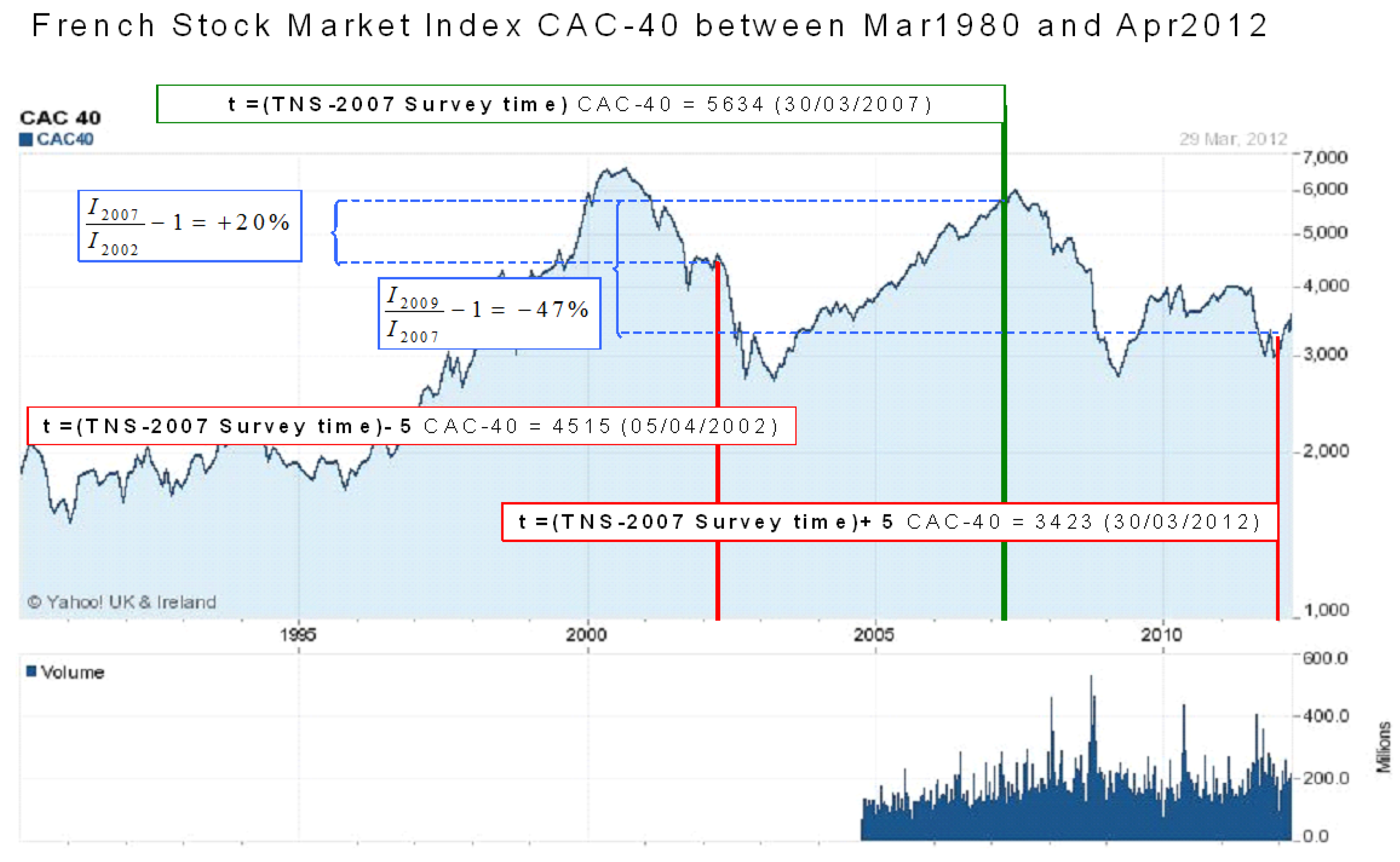
9
The CAC-40 takes its name from the Paris Bourse’s (today called Euronext Paris) early automation system “Cotation Assistée en Continu” (Continuous Assisted Quotation). Its base value of 1000 was set on the 31 December 1987, equivalent to a market capitalisation of 370,437,433,957.70 FF.
10
Those respondents are also more likely to form a rational expectation from an adaptive learning viewpoint (see Evans and Honkapohja 2001).
11
We follow the standard convention in finance for long-horizon returns (e.g., Campbell et al. 1997), and let 1 + R t + 1 ( s ) denote the stock market index gross return over s periods ahead; (hence, the subindex t + 1 ), which is equal to the product of the s single-period (or yearly) returns:
1 + R t + 1 ( s ) = f = 0 s 1 ( 1 + R t + 1 + f ) = f = 0 s 1 I t + 1 + f I t + f
Similarly, we let 1 + R t ( s ) denote the stock market index gross return over the most recent s periods from date t s to date t (hence the subindex t):
1 + R t ( s ) = b = 0 s 1 ( 1 + R t b ) = b = 0 s 1 I t b I t 1 b
12
Because these bounds are commonly missing from surveys collecting respondents’ subjective expectations, researchers opt for ’winsorising’ the support of the outcome variable to guard against outliers. Results from experimenting with ± 50 and ± 100 percent bounds are very similar to those reported below, and are therefore omitted for brevity but available upon request.
13
When missing and erroneous answers are regressed against stockholding status, and a set of covariates (gender, education, risk preferences), they appear strongly related to stock holdings, just as Kézdi and Willis (2009) find for the HRS 2002 wave. Results are available from the authors upon request.
14
According to Glaser et al. (2019) if instead we had exploited a ’price elicitation format’ for the CAC-40 index (rather than its percentage change, or return), we would have obtained even lower mean expected cumulative stock market returns.
15
Ex-post, Figure 1 reveals that by March 2012 the CAC-40 index was down by 47% relative to March 2007. However, by March 2007, the French market did not anticipate the 2007–2009 US stock market crash, during which the S&P500 lost more than 50% of its value, triggering the Great Recession.
16
Most of the recent empirical literature focusing on perceptions only elicits point answers from respondents (e.g., Armona et al. 2019; Kumar et al. 2015 or Coibion et al. 2018).
17
Arrondel et al. (2014) show that conditioning on perceived realised returns also reduces the ’heaping’ around focal point responses conveying absolute certainty.
18
Similar findings are reported in Armantier et al. (2016) and Coibion et al. (2018) for households’ and firms’ perceptions about inflation, respectively.
19
We exclude both government bonds and home ownership from the risky asset category, even if the latter are highly illiquid and indivisible (and therefore risky), because French households mostly buy houses for the flow of services they provide rather than as a financial investment. Still, in the estimation, we control for the level of total wealth (real plus financial), and include a dummy variable that takes value one when home-ownership status is observed.
20
The results of the econometric specifications in logarithmic form are unreported, but available from the authors upon request.
21
The results are robust to an alternative measure of risk aversion: the coefficient of relative risk aversion for preferences in the constant relative risk aversion class (CRRA), advanced by Barsky et al. (1997) and available in the TNS 2007 survey wave. In addition, Kimball et al. (2008) show that the CRRA measure is robust to survey measurement error. The results are available from the authors upon request.
22
Our measure of temporal preference is inversely proportional to “impatience”, or how far-sighted the respondent is, rather than a preference for an early resolution of uncertainty, as in Van Nieuwerburgh and Veldkamp (2010).
23
See King and Leape (1998) and simulated results by Haliassos and Michaelides (2003).
24
If we were interested in a continuous measure, we would implement the method of simulated residuals by Gourieroux et al. (1987). We would then regress an ordered probit of the respondents’ total wealth (bracket) on demographic and socioeconomic household characteristics. Once we would have the estimated total wealth, a normally distributed error would be added. We would then check if the value falls inside the bracket originally chosen by the individual. If not, another normal error would be added and so on until we the true interval is correctly predicted. Doing so would allow us to overcome the non-response problem for some households. Would there be a missing value, the predicted value plus a normal error would be directly used.
25
In France, income is not taxed at the source.

References

  1. Abel, Andrew B., Janice C. Eberly, and Stavros Panageas. 2007. Optimal Inattention to the Stock Market. American Economic Review 97: 244–49. [Google Scholar] [CrossRef] [Green Version]
  2. Abel, Andrew, Janice Eberly, and Stavros Panageas. 2013. Optimal Inattention to the Stock Market With Information Costs and Transactions Costs. Econometrica 81: 1455–81. [Google Scholar]
  3. Alvarez, Fernando, Luigi Guiso, and Francesco Lippi. 2012. Durable Consumption and Asset Management With Transaction and Observation Costs. American Economic Review 102: 2272–300. [Google Scholar] [CrossRef] [Green Version]
  4. Ambuehl, Sandro, B. Douglas Bernheim, and Annamaria Lusardi. 2021. Evaluating Deliberative Competence: A Simple Method with an Application to Financial Choice. Available online: https://drive.google.com/file/d/133oh2OC-EeBtOsXusPsMLQ9YFB-gyZJP/view?usp=sharing (accessed on 27 November 2021).
  5. Ameriks, John, Gábor Kézdi, Minjoon Lee, and Matthew D. Shapiro. 2020. Heterogeneity in Expectations, Risk Tolerance, and Household Stock Shares: The Attenuation Puzzle. Journal of Business and Economic Statistics 38: 633–46. [Google Scholar] [CrossRef]
  6. Amromin, Gene, and Steven A. Sharpe. 2013. From the Horse’s Mouth: Economic Conditions and Investor Expectations of Risk and Return. Management Science 60: 845–66. [Google Scholar] [CrossRef]
  7. Andrade, Phillipe, and Herve Le Bihan. 2013. Inattentive Professional Forecasters. Journal of Monetary Economics 11: 967–82. [Google Scholar] [CrossRef] [Green Version]
  8. Armantier, Olivier, Scott Nelson, Giorgio Topa, Wilbert Van der Klaauw, and Basit Zafar. 2016. The Price is Right: Updating Inflation Expectations in a Randomized Price Information Experiment. Review of Economics and Statistics 98: 503–23. [Google Scholar] [CrossRef]
  9. Armona, Luis, Andreas Fuster, and Basit Zafar. 2019. Home Price Expectations and Behaviour: Evidence from a Randomized Information Experiment. Review of Economic Studies 86: 1371–410. [Google Scholar] [CrossRef]
  10. Arrondel, Lucarrdo, Hector F. Calvo Pardo, and Derya Tas. 2014. Subjective Return Expectations, Information and Stock Market Participation: Evidence from France. Southampton: University of Southampton Economics. [Google Scholar]
  11. Arrow, Kenneth Joseph. 1965. Aspects of the Theory of Risk Bearing. Yrjo Jahnsson Lectures. Helsinki: The Academic Book Store. [Google Scholar]
  12. Badarinza, Cristian, John Y. Campbell, and Tarun Ramadorai. 2016. International Comparative Household Finance. Annual Review of Economics 8: 111–44. [Google Scholar] [CrossRef] [Green Version]
  13. Barsky, Robert B., F. Thomas Juster, Miles S. Kimball, and Matthew D. Shapiro. 1997. Preference Parameters and Behavioral Heterogeneity: An Experimental Approach in the Health and Retirement Study. Quarterly Journal of Economics CXII: 537–80. [Google Scholar]
  14. Bilias, Yannis, Dimitris Georgarakos, and Mithael Haliassos. 2010. Portfolio Inertia and Stock Market Fluctuations. Journal of Money, Credit and Banking 42: 715–42. [Google Scholar] [CrossRef] [Green Version]
  15. Biais, Bruno, Peter Bossaerts, and Chester Spatt. 2010. Equilibrium Asset Pricing and Portfolio Choice Under Asymmetric Information. Review of Financial Studies 23: 1503–43. [Google Scholar] [CrossRef]
  16. Bordalo, Pedro, Nicola Gennaioli, and Andei Shleifer. 2018. Diagnostic Expectations and Credit Cycles. Journal of Finance 73: 199–227. [Google Scholar] [CrossRef]
  17. Brandt, Michael W. 2010. Portfolio Choice Problems. In Handbook of Financial Econometrics, Volume 1: Tools and Techniques. Edited by Yacine Aït-Sahalia and Lars Peter Hansen. Amsterdam: Elsevier North-Holland. [Google Scholar]
  18. Campbell, John Y. 2006. Household Finance. The Journal of Finance 61: 1553–604. [Google Scholar] [CrossRef] [Green Version]
  19. Campbell, John Y. 2016. Restoring Rational Choice: The Challenge of Consumer Financial Regulation. American Economic Review: Papers & Proceedings 106: 1–30. [Google Scholar]
  20. Campbell, John Y., Andrew W. Lo, and A. Craig MacKinlay. 1997. The Econometrics of Financial Markets. Princeton: Princeton University Press. [Google Scholar]
  21. Carroll, Cristopher D. 2017. Heterogeneity, Macroeconomics, and Reality. Paper presented at the Keynote Lecture, Sloan-Bank of England-Office of Financial Research Conference on Heterogeneous Agent Macroeconomics, Washington, DC, USA, September 22. [Google Scholar]
  22. Christelis, Dimitris, Tullio Jappelli, and Mario Padula. 2010. Cognitive Abilities and Portfolio Choice. European Economic Review 54: 18–38. [Google Scholar] [CrossRef] [Green Version]
  23. Christelis, Dimitris, Dimitris Georgarakos, Tullio Jappelli, and Maarten van Rooij. 2020. Consumption Uncertainty and Precautionary Savings. The Review of Economics and Statistics 10: 148–61. [Google Scholar] [CrossRef] [Green Version]
  24. Coibion, Olivier, Yuriy Gorodnichenko, and Saten Kumar. 2018. How Do Firms Form Their Expectations? New Survey Evidence. American Economic Review 108: 2671–713. [Google Scholar] [CrossRef] [Green Version]
  25. Dimson, Elroy, Paul Marsh, and Mike Staunton. 2012. Equity premiums around the world. In Rethinking the Equity Premium. Edited by Brett Hammond, Martin Leibowitz and Laurence Siegel. Charlottesville: Research Foundation of the CFA Institute, chp. 4. pp. 32–52. [Google Scholar]
  26. Dominitz, Jeff, and Charles F. Manski. 2007. Expected Equity Returns and Portfolio Choice: Evidence from the Health and Retirement Study. Journal of the European Economic Association 5: 369–79. [Google Scholar] [CrossRef]
  27. Dominitz, Jeff, and Charles Manski. 2011. Measuring and Interpreting Expectations of Equity Returns. Journal of Applied Econometrics 26: 352–70. [Google Scholar] [CrossRef] [Green Version]
  28. Donkers, Bas, and Arthur van Soest. 1999. Subjective measures of household preferences and financial decisions. Journal of Economic Psychology 20: 613–42. [Google Scholar] [CrossRef]
  29. Dow, James, and Sergio Ribeiro da Costa Werlang. 1992. Uncertainty Aversion, Risk Aversion, and the Optimal Choice of Portfolio. Econometrica 60: 197–204. [Google Scholar] [CrossRef]
  30. Duffie, Darrell, and Tong-Sheng Sun. 1990. Transactions Costs and Portfolio Choice in a Discrete-Continuous Time Setting. Journal of Economic Dynamics & Control 14: 35–51. [Google Scholar]
  31. Evans, George W., and Seppo Honkapohja. 2001. Learning and Expectations in Macroeconomics. Princeton: Princeton U. Press. [Google Scholar]
  32. Fagereng, Andreas, Charles Gottlieb, and Luigi Guiso. 2017. Asset Market Participation and Portfolio Choice over the Life-Cycle. Journal of Finance 72: 705–50. [Google Scholar] [CrossRef] [Green Version]
  33. Gennotte, Gerard. 1986. Optimal Portfolio Choice Under Incomplete Information. Journal of Finance 61: 733–46. [Google Scholar] [CrossRef]
  34. Giglio, Stefano, Matteo Maggiori, Johannes Stroebel, and Stephen Utkus. 2021. Five Facts about Beliefs and Portfolios. American Economic Review 111: 1481–522. [Google Scholar] [CrossRef]
  35. Glaser, Markus, Zwetelina Iliewa, and Martin Weber. 2019. Thinking about Prices versus Thinking about Returns in Financial Markets. Journal of Finance 74: 2997–3039. [Google Scholar] [CrossRef]
  36. Gourieroux, Christian, Alain Monfort, Eric Renault, and Alain Trognon. 1987. Simulated Residuals. Journal of Econometrics 34: 201–52. [Google Scholar] [CrossRef]
  37. Gomes, Francisco, Michael Haliassos, and Tarun Ramadorai. 2021. Household Finance. Journal of Economic Literature 59: 91–1000. [Google Scholar] [CrossRef]
  38. Grinblatt, Mark, Matti Keloharju, and Juhani Linnainmaa. 2011. IQ and Stock Market Participation. The Journal of Finance 66: 2121–64. [Google Scholar] [CrossRef]
  39. Guesnerie, Roger. 1992. An Exploration of the Eductive Justifications of the Rational Expectations Hypothesis. American Economic Review 82: 1254–78. [Google Scholar]
  40. Guiso, Luigi, and Monica Paiella. 2008. Risk Aversion, Wealth and Background Risk. Journal of the European Economic Association 6: 1109–150. [Google Scholar] [CrossRef]
  41. Guiso, Luigi, and Paolo Sodini. 2013. Household Finance: An Emerging Field. In Handbook of the Economics of Finance. Edited by George Constandinides, Milton Harris and Rene Stulz. Amsterdam: Elsevier Science, vol. 2B, pp. 1397–531. [Google Scholar]
  42. Guiso, Luigi, Tullio Jappelli, and Daniele Terlizzese. 1996. Income risk, borrowing constraints and portfolio choice. American Economic Review 86: 158–72. [Google Scholar]
  43. Guiso, Luigi, Michael Haliassos, and Tullio Jappelli. 2002. Household Portfolios. Cambridge: MIT Press. [Google Scholar]
  44. Haliassos, Michael. 2008. Household Portfolios. In The New Palgrave Dictionary of Economics. Edited by Steven N. Durlauf and Lawrence E. Blume. The New Palgrave Dictionary of Economics Online. London: Palgrave Macmillan. [Google Scholar]
  45. Haliassos, Michael, and Caro C. Bertaut. 1995. Why Do So Few Hold Stocks? Economic Journal 105: 1110–29. [Google Scholar] [CrossRef]
  46. Haliassos, Michael, and Alexander Michaelides. 2003. Portfolio Choice and Liquidity Constraints. International Economic Review 44: 143–78. [Google Scholar] [CrossRef]
  47. Hurd, Michael D. 2009. Subjective Probabilities in Household Surveys. Annual Review of Economics 1: 543–62. [Google Scholar] [CrossRef] [Green Version]
  48. Hurd, Michael D., Maarten van Rooij, and Joachim Winter. 2011. Stock Market Expectations of Dutch Households. Journal of Applied Econometrics 26: 416–36. [Google Scholar] [CrossRef] [Green Version]
  49. Jonung, Lars, and David Laidler. 1988. Are Perceptions of Inflation Rational? Some Evidence for Sweden. American Economic Review 78: 1080–87. [Google Scholar]
  50. Kézdi, Gabor, and Robert J. Willis. 2009. Stock Market Expectations and Portfolio Choice of American Households. Available online: https://www.researchgate.net/publication/228820548_Stock_market_expectations_and_portfolio_choice_of_American_Households (accessed on 10 December 2021).
  51. Kimball, Miles S., Claudia R. Sham, and Matthew D. Shapiro. 2008. Imputing Risk Tolerance from Survey Responses. Journal of the American Statistical Association 103: 1028–38. [Google Scholar] [CrossRef] [PubMed] [Green Version]
  52. King, Mervyn A., and Jonathan I. Leape. 1998. Wealth and portfolio composition: Theory and Evidence. Journal of Public Economics 69: 155–93. [Google Scholar] [CrossRef] [Green Version]
  53. Klein, Roger W., and Vijay S. Bawa. 1976. The Effect of Estimation Risk on Optimal Portfolio Choice. Journal of Financial Economics 3: 215–32. [Google Scholar] [CrossRef]
  54. Koijen, Ralph S. J., and Motohiro Yogo. 2019. A Demand System Approach to Asset Pricing. Journal of Political Economy 127: 1475–515. [Google Scholar] [CrossRef] [Green Version]
  55. Kuhnen, Camelia M. 2015. Asymmetric Learning from Financial Information. Journal of Finance 70: 2029–62. [Google Scholar] [CrossRef] [Green Version]
  56. Kumar, Saten, Hassan Afrouzi, Olivier Coibion, and Yuriy Gorodnichenko. 2015. Inflation Targeting Does Not Anchor Inflation Expectations: Evidence From Firms in New Zealand. Brookings Papers on Economic Activity 2015: 151–208. [Google Scholar]
  57. Le Bris, David, and Pierre-Cyrille Hautcoeur. 2010. A challenge to triumphant optimists? A blue chips index for the Paris stock exchange, 1854–2007. Financial History Review 17: 141–183. [Google Scholar] [CrossRef] [Green Version]
  58. Lusardi, Annamaria, Pierre-Cyrrile Michaud, and Olivia S. Mitchell. 2017. Optimal Financial Knowledge and Wealth Inequality. Journal of Political Economy 125: 431–77. [Google Scholar] [CrossRef] [Green Version]
  59. Lusardi, Annamaria, and Olivia S. Mitchell. 2014. The Economic Importance of Financial Literacy: Theory and Evidence. Journal of Economic Literature 52: 5–44. [Google Scholar] [CrossRef] [Green Version]
  60. Malmendier, Ulrike, and Stefan Nagel. 2011. Depression Babies: Do Macroeconomic Experiences Affect Risk Taking? The Quarterly Journal of Economics 126: 373–416. [Google Scholar] [CrossRef] [Green Version]
  61. Malmendier, Ulrike, and Stefan Nagel. 2016. Learning from inflation Experiences. The Quarterly Journal of Economics 131: 53–87. [Google Scholar] [CrossRef]
  62. Manski, Charles. 2004. Measuring Expectations. Econometrica 72: 1329–76. [Google Scholar] [CrossRef]
  63. Manski, Charles. 2018. Survey Measurement of Probabilistic Macroeconomic Expectations: Progress and Promise. NBER Macroeconomics Annual 32: 411–71. [Google Scholar] [CrossRef] [Green Version]
  64. Merkoulova, Yulia, and Chris Veld. 2021. Stock Return Ignorance. Journal of Financial Economics. [Google Scholar] [CrossRef]
  65. Merton, Robert C. 1969. Lifetime Portfolio Selection under Uncertainty: The Continuous Time Case. Review of Economics and Statistics 51: 247–57. [Google Scholar] [CrossRef] [Green Version]
  66. Miniaci, Raffaele, and Sergio Pastorello. 2010. Mean–Variance Econometric Analysis of Household Portfolios. Journal of Applied Econometrics 25: 481–504. [Google Scholar] [CrossRef]
  67. Pástor, Lubos, and Pietro Veronesi. 2009. Learning in Financial markets. Annual Review of Financial Economics 1: 361–81. [Google Scholar] [CrossRef] [Green Version]
  68. Reis, Ricardo. 2006. Inattentive Consumers. Journal of Monetary Economics 53: 1761–800. [Google Scholar] [CrossRef]
  69. Samuelson, Paul A. 1969. Lifetime Portfolio Selection by Dynamic Stochastic Programming. Review of Economics and Statistics 51: 239–46. [Google Scholar] [CrossRef]
  70. Sims, Christopher. 2003. Implications of Rational Inattention. Journal of Monetary Economics 50: 665–90. [Google Scholar] [CrossRef] [Green Version]
  71. Tufano, Peter. 2009. Consumer Finance. Annual Review of Financial Economics 1: 227–47. [Google Scholar] [CrossRef]
  72. Van Nieuwerburgh, Stijn, and Laura Veldkamp. 2010. Information Acquisition and Under-Diversification. Review of Economic Studies 77: 779–805. [Google Scholar] [CrossRef] [Green Version]
  73. van Rooij, Maarten, Annamaria Lusardi, and Rob Alessie. 2011. Financial Literacy and Stock Market Participation. Journal of Financial Economics 101: 449–72. [Google Scholar] [CrossRef] [Green Version]
  74. Vissing-Jorgensen, Annette. 2002. Towards and Explanation of Household Portfolio Choice Heterogeneity: Nonfinancial Income and Participation Cost Structures. Cambridge: NBER WP. [Google Scholar]
  75. Vissing-Jorgensen, Annette. 2004. Perspectives on Behavioural Finance: Does Irrationality Disappear with Wealth? Evidence from Expectations and Actions. In The NBER Macroeconomics Annual 2003. Edited by Mark Gertler and Kenneth Rogoff. Cambridge: MIT Press. [Google Scholar]
  76. Woodford, Michael. 2013. Macroeconomic Analysis without the Rational Expectations Hypothesis. Annual Review of Economics 5: 303–46. [Google Scholar] [CrossRef] [Green Version]
  77. Zhang, X. Frank. 2006. Information Uncertainty and Stock Market Returns. The Journal of Finance 61: 105–37. [Google Scholar] [CrossRef]
Figure 1. The French Stock Market Index CAC-40 between March 1980 and April 2012. Between March 2002 (first vertical red bar, 5 years prior to the time of the survey) and March 2007 (vertical green bar, survey administration time) the index had increased by around 20%, while between March 2007 and March 2012 (5 years after the time of the survey, second vertical red bar) the index had dropped by around 47%. Source: author’s calculations from Yahoo Finance monthly data, available online.
Jrfm 15 00006 g001
Figure 2. Histogram of average individual answers to the likelihood of the different scenarios regarding 5-year ahead cumulative stock market returns. Source: TNS 2007 survey.
Jrfm 15 00006 g002
Figure 3. Individual histograms of responses to the most recent five-year cumulative stock market return realisation, survey question (qc9). Source: TNS2007.
Jrfm 15 00006 g003
Figure 4. Histogram of average individual answers to the relative likelihood of the different scenarios regarding the most recent five-year cumulative stock market return realisation, survey question (qc9). Source: TNS2007.
Jrfm 15 00006 g004
Table 1. 2007 TNS Descriptive Statistics.
Overall SampleEstimation SampleNR(PR) = 0NR(PR) = 1
VariablesMeanSdMeanSdMeanSdMeanSd
Share of fin. wealth in stocks0.2890.4530.450.4980.4660.4990.3360.473
Direct or indirect stockholdings26.625.12725.427.125.425.925.6
Share of fin. wealth in stocks?11.120.912.121.712.6228.7119.2
Exp. Ret. (ER)0.03560.09410.05890.1090.06240.1080.03460.11
Sd. Exp. Ret. (Sd ER)0.04370.06730.06970.07280.07110.07240.060.0745
Mean Perc. cum. Ret. (PR)0.06960.1220.110.1370.1250.1400
Sd. Perc. cum. Ret. (Sd PR)0.03830.0620.05750.06730.06570.068100
Risk aversion (CARA)34.213.437.97.42387.0737.29.49
NR(CARA) = 00.8740.3320.9730.1630.9770.150.9410.235
Temporal pref.6.612.516.792.256.772.236.922.41
Age48.31.6846.71.5646.61.5447.21.65
Male0.540.4980.490.50.490.50.550.498
Having children0.7470.4350.7360.4410.7420.4370.6880.464
Paris region (residence)0.1690.3750.1910.3930.1930.3950.1760.381
Trust0.4570.4980.5530.4970.5720.4950.4220.495
Educational attainment:
High school0.0805 0.0425 0.0369 0.082
Technical/Professional0.0672 0.0474 0.0447 0.0664
Some/college0.6223 0.6158 0.6134 0.6328
More than college0.23 0.2942 0.305 0.2188
Income (survey brackets):
NR(Income) = 10.0876 0.0435 0.0402 0.0664
Income < 80000.1673 0.1305 0.1251 0.168
8000 < Income < 11,9990.126 0.1031 0.0994 0.1289
12,000 < Income < 15,9990.1673 0.154 0.1497 0.1836
16,000 < Income < 19,9990.1545 0.1745 0.1765 0.1602
20,000 < Income < 39,9990.1955 0.2434 0.252 0.1836
40,000 < Income < 59,9990.0677 0.0958 0.1011 0.0586
Income > 60,0000.0342 0.0552 0.0559 0.0508
Wealth (survey brackets):
NR(Wealth) = 10.1691 0.0523 0.0447 0.1055
Wealth < 80000.1328 0.1139 0.1056 0.1719
8000 < Wealth < 14,9990.0442 0.042 0.0408 0.0508
15,000 < Wealth < 39,9990.0591 0.0689 0.0704 0.0586
40,000 < Wealth < 74,9990.0502 0.0557 0.0553 0.0586
75,000 < Wealth < 149,9990.1325 0.1364 0.1385 0.1211
150,000 < Wealth < 224,9990.1553 0.1779 0.1788 0.1719
225,000 < Wealth < 299,9990.0978 0.129 0.1307 0.1172
300,000 < Wealth < 449,9990.0917 0.1246 0.1313 0.0781
450,000 < Wealth < 749,9990.051 0.0743 0.0782 0.0469
Wealth > 750,0000.0165 0.0249 0.0257 0.0195
Liquidity constrained0.02250.1480.01420.1180.01280.1130.02340.152
Irregular income0.2060.4040.1970.3980.1970.3980.1990.4
Online banking0.4110.4920.4980.50.5080.50.4260.495
Intergenerational transf.0.4720.5990.5030.610.5180.6170.4020.551
Parents own risky assets0.260.4390.3270.4690.3410.4740.2340.424
Firm shares in remuneration0.04730.2120.05910.2360.06030.2380.05080.22
Enjoys managing finances0.07110.2570.0890.2850.09270.290.06250.243
N382620461790256
Notes: This table reports descriptive statistics for the overall sample of 3826 respondents to the 2007 TNS survey wave (cols. 1–2) and for the estimation sample (cols. 3–4) of 2046 respondents to the (direct and indirect) stockholdings (qc14) and return expectations (qc6, qc9) questions, separating respondents (cols. 5–6) from nonrespondents (cols. 7–8) to the return perceptions questions (qc9). Questions about returns enable quantitative elicitation of households’ beliefs over a five-year horizon (Manski 2004). Risk aversion is elicited following the methodology of Guiso and Paiella (2008). Temporal preference is a qualitative 11-point Likert scale measuring how much the respondent cares about the future (qi18) with ‘0’ denoting ‘impatience’ and ‘10’ ‘patient’. Wealth and annual Income brackets expressed in EUR. The rest of the variables are detailed in the Appendix A.
Table 2. Survey Responses to Expectations and Perceptions of Cumulative Stock Market Returns Questions.
VariablesMeanStandard Deviation (Sd)25th PercentileMedian75th PercentileN
Overall sample:
Exp. cum. Ret. (ER)0.05530.11300.02110.12460
Sd. Exp. cum. Ret. (Sd ER)0.0680.073500.050.122460
Mean Perc. cum. Ret. (PR)0.1190.140.010.09250.1832231
Sd. Perc. cum. Ret. (Sd PR)0.06560.069200.050.1152231
Estimation sample:
Exp. cum. Ret. (ER)0.05890.10900.0250.1052046
Sd. Exp. cum. Ret. (Sd ER)0.06970.072800.05260.1232046
Mean Perc. cum. Ret. (PR)0.1250.140.01880.1020.191790
Sd. Perc. cum. Ret. (Sd PR)0.06570.068100.05250.1151790
Notes: ER is expected five-year ahead cumulative returns of the stock market index CAC40, and Sd ER is its standard deviation; PR is the perception of realised cumulative returns of the stock market index CAC40 over the five years immediately preceding the 2007 TNS survey administration date (March 2007), and Sd PR is its standard deviation; N denotes the number of valid survey responses out of the overall (3826) and estimation (2039) samples
Table 3. Subjective Stock Market Return Expectations and Stockholdings.
No ExpectationsWith ExpectationsExpectations (Two-Step) 
Variables [1] [2] [3] [4] [5] [6]
Exp. Ret. (ER) 0.355 ***7.2830.722 **54.084 **
(0.093)(9.202)(0.266)(25.895)
Sd. Exp. Ret. (Sd ER) 0.478 ***−36.377 **0.152−36.640 *
(0.139)(12.278)(0.260)(21.600)
Risk aversion (CARA)−0.003−0.262−0.002−0.296−0.001−0.191
(0.003)(0.203)(0.003)(0.198)(0.003)(0.205)
Temporal pref.0.013 **−0.990 **0.012 **−0.962 **0.012 **−1.006 **
(0.005)(0.482)(0.005)(0.470)(0.005)(0.466)
Trust0.049 **−3.656 *0.047 *−3.734 *0.041 *−4.043 *
(0.024)(2.190)(0.024)(2.173)(0.024)(2.159)
Income < 8000−0.094−0.884−0.09−0.2−0.0820.088
(0.058)(5.897)(0.058)(5.721)(0.057)(5.785)
8000 < Income < 11,9990.016−3.4890.025−2.5510.036−1.367
(0.059)(5.696)(0.059)(5.574)(0.059)(5.670)
12,000 < Income < 19,9990.011−3.2460.019−2.5250.026−1.787
(0.056)(5.356)(0.056)(5.227)(0.056)(5.277)
20,000 < Income < 29,9990.017−7.460.023−6.6970.033−5.537
(0.056)(5.275)(0.056)(5.122)(0.056)(5.240)
30,000 < Income < 39,9990.049−6.4140.048−5.6830.048−5.582
(0.055)(5.199)(0.055)(5.058)(0.055)(5.108)
40,000 < Income < 59,9990.052−3.8340.06−3.1860.065−2.692
(0.062)(5.740)(0.062)(5.580)(0.062)(5.639)
Income > 60,0000.056−2.8670.054−2.050.059−1.642
(0.072)(6.008)(0.071)(5.864)(0.071)(5.908)
Wealth < 8000−0.0769.398−0.0797.368−0.0886.017
(0.056)(6.418)(0.056)(6.309)(0.056)(6.391)
8000 < Wealth < 14,999016.235 **0.00915.392 **0.00715.769 **
(0.069)(7.419)(0.069)(7.374)(0.070)(7.267)
15,000 < Wealth < 39,9990.0555.20.0564.6360.0534.142
(0.062)(5.696)(0.062)(5.562)(0.062)(5.471)
40,000 < Wealth < 74,9990.111 *4.890.115 *4.1170.1033.82
(0.065)(5.654)(0.065)(5.648)(0.065)(5.604)
75,000 < Wealth < 149,9990.077−2.1890.079−2.6770.069−3.203
(0.055)(4.407)(0.055)(4.362)(0.055)(4.332)
150,000 < Wealth < 224,9990.105 **1.8210.108 **1.0870.102 *1.008
(0.054)(4.339)(0.053)(4.310)(0.053)(4.288)
225,000 < Wealth < 299,9990.103 *6.150.108 *5.3450.102 *5.673
(0.056)(4.735)(0.056)(4.712)(0.056)(4.706)
300,000 < Wealth < 449,9990.290 ***−0.2580.287 ***−0.6790.276 ***−0.83
(0.057)(5.031)(0.057)(5.019)(0.057)(4.996)
450,000 < Wealth < 749,9990.221 ***0.80.217 ***0.4880.208 **0.05
(0.064)(5.299)(0.064)(5.224)(0.064)(5.191)
Wealth > 750,0000.498 ***−1.7180.496 ***−1.5890.485 ***−2.19
(0.077)(7.013)(0.078)(7.049)(0.079)(6.955)
Female−0.011−2.267−0.005−2.1810.001−1.163
(0.022)(1.826)(0.022)(1.799)(0.022)(1.910)
Age0.0345.2980.0295.3790.0325.681
(0.043)(3.694)(0.043)(3.612)(0.043)(3.622)
Age squared−0.001−0.470−0.498−0.001−0.527
(0.004)(0.355)(0.004)(0.347)(0.004)(0.349)
High school0.184 **3.7850.192 **4.3870.191 **5.031
(0.067)(6.220)(0.066)(6.233)(0.066)(6.201)
Technical/Professional0.0712.5790.082.6680.0772.77
(0.053)(4.720)(0.052)(4.662)(0.052)(4.637)
Some/college0.0722.2760.082.660.0792.909
(0.056)(5.021)(0.056)(4.963)(0.056)(4.947)
Having children−0.029 −0.022 −0.021
(0.027) (0.026) (0.027)
Paris region (residence)0.026 0.016 0.013
(0.027) (0.027) (0.027)
Parents own risky assets0.134 *** 0.130 *** 0.126 ***
(0.022) (0.022) (0.022)
Firm shares in remuneration0.193 *** 0.192 *** 0.192 ***
(0.044) (0.044) (0.044)
Intergenerational transf.0.059 ** 0.059 ** 0.060 ***
(0.018) (0.018) (0.018)
Liquidity constrained                   −0.203 *−3.748−0.186 *−4.562−0.169−1.88
(0.107)(12.225)(0.106)(12.456)(0.106)(12.121)
Irregular income0.0294.639 *0.0284.584 *0.0284.668 *
(0.028)(2.660)(0.028)(2.636)(0.028)(2.633)
Online banking0.0225.036 **0.0185.102 **0.0164.613 **
(0.024)(2.092)(0.024)(2.060)(0.024)(2.033)
NR(CARA)0.07213.3210.01814.7620.00110.227
(0.125)(9.180)(0.126)(9.081)(0.128)(9.359)
Residuals (ER) −0.427−52.115 **
(0.285)(25.924)
Residuals (Sd ER) 0.4672.051
(0.307)(25.549)
Mills ratio −9.419 * −7.728 −6.041
(5.441) (5.593) (5.678)
N203920392039
1 Notes: Marginal effects from Heckman regressions of probits for stock market participation (odd-numbered cols.) and estimated coefficients of regression on the share of financial wealth invested in the stock market (direct or indirect), conditional on investing (even-numbered cols.), without (cols. 1–2), and with empirical (cols. 3–6) first and second moments of subjective expectations of returns, including covariates for: (a) Preferences for risk and time (patience); (b) Demographics: age, gender and children at home; (c) Information proxies: trust, education, region of residence; (d) Endowments: total wealth and income survey brackets; (e) Constraints: access to online banking, irregular income and borrowing/liquidity constrained status; (f) Inertial factors: inter vivos/mortis causa transfers received, parental stockownership and firm shares in remuneration status, separately identifying the extensive from the intensive margin (first exclusion restriction); and (g) Residuals from the first-stage first and second moment regressions (reported in Table 4, cols. 1–2), enabling the control function approach (second exclusion restriction). Non-responses (NR) to the risk aversion question category included, NR(CARA). Reference categories are: Male, less than high school education, non-respondents to income and wealth questions, not living in Paris, parents not owning stocks, no firm shares in remuneration, no intergenerational transfers received, regular or partly regular income, borrowing and liquidity unconstrained, no access to online banking. Wealth and annual Income brackets expressed in EUR. A constant term is included but not reported. Bootstrapped standard errors are reported in parentheses (10,000 replications). ***, ** and * denote significance at 1%, 5% and 10%, respectively. Source: TNS2007 wave, France.
Table 4. Subjective Expectations and Perceptions of Cumulative Stock Market Returns.
Exp. Ret. (ER)Sd. Exp. Ret. (Sd ER)Mean Perc. Ret. (PR)Sd. Perc. Ret. (Sd PR)
Variables [1] [2] [3] [4]
Mean Perc. cum. Ret. (PR)0.292 ***0.008
(0.022)(0.012)
Sd. Perc. cum. Ret. (Sd PR)0.0270.608 ***
(0.034)(0.024)
NR(PR) = 1−0.015 *−0.031 ***
(0.008)(0.005)
Enjoys managing finances0.024 **0.001
(0.009)(0.005)
Risk aversion (CARA)−0.002 *−0.001 ***−0.0010
(0.001)(0.000)(0.001)(0.000)
Temporal pref.000.0010
(0.001)(0.001)(0.001)(0.001)
Trust0.007−0.0030.018 **0.001
(0.006)(0.003)(0.007)(0.004)
Income < 8000−0.020.0010.0110.01
(0.018)(0.008)(0.016)(0.009)
8000 < Income < 11,999−0.031 *0.0010.0160.013
(0.018)(0.008)(0.016)(0.009)
12,000 < Income < 19,999−0.023−0.0060.0130.015 *
(0.017)(0.008)(0.016)(0.008)
20,000 < Income < 29,999−0.02300.0060.013
(0.018)(0.008)(0.016)(0.008)
30,000 < Income < 39,999−0.009−0.0020.033 **0.013
(0.017)(0.008)(0.016)(0.008)
40,000 < Income < 59,999−0.022−0.0030.0220.005
(0.018)(0.009)(0.018)(0.009)
Income > 60,000−0.0220.0050.056 **0.004
(0.020)(0.010)(0.020)(0.010)
Wealth < 80000.009−0.0140.035 **0.007
(0.013)(0.009)(0.014)(0.008)
8000 < Wealth < 14,999−0.017−0.0150.0270.001
(0.015)(0.010)(0.017)(0.010)
15,000 < Wealth < 39,999−0.008−0.0090.038 **0.01
(0.013)(0.009)(0.017)(0.009)
40,000 < Wealth < 74,9990.001−0.020 **0.039 **0.003
(0.015)(0.009)(0.018)(0.010)
75,000 < Wealth < 149,9990.005−0.015 *0.034 **0.008
(0.013)(0.008)(0.014)(0.008)
150,000 < Wealth < 224,999−0.003−0.0110.037 **0.003
(0.011)(0.008)(0.014)(0.008)
225,000 < Wealth < 299,999−0.001−0.014 *0.0150.007
(0.012)(0.008)(0.015)(0.008)
300,000 < Wealth < 449,9990.006−0.0080.050 **0.002
(0.012)(0.008)(0.015)(0.008)
450,000 < Wealth < 749,9990.007−0.0070.036 **0.009
(0.015)(0.009)(0.018)(0.009)
Wealth > 750,0000.015−0.0130.064 **0.013
(0.020)(0.013)(0.024)(0.012)
Female−0.006−0.007 **−0.041 ***0.007 **
(0.005)(0.003)(0.006)(0.003)
Age−0.0020.0080.0160.005
(0.010)(0.006)(0.012)(0.006)
Age squared0−0.001 *0−0.001
(0.001)(0.001)(0.001)(0.001)
High school−0.0140.0020.025−0.012
(0.017)(0.010)(0.021)(0.011)
Technical/Professional−0.011−0.010.012−0.003
(0.014)(0.008)(0.017)(0.009)
Some/college−0.013−0.0060.019−0.004
(0.015)(0.008)(0.018)(0.010)
Having children−0.006−0.008 **−0.0030
(0.006)(0.004)(0.007)(0.004)
Paris region (residence)0.013 **0.008 **0.013 *0.001
(0.006)(0.004)(0.008)(0.004)
Parents own risky assets0.0080.005 *0.011 *−0.007 **
(0.005)(0.003)(0.007)(0.003)
Firm shares in remuneration−0.001−0.0010.0110.001
(0.009)(0.005)(0.013)(0.006)
Intergenerational transf.−0.0020.0010.011 *0.002
(0.004)(0.002)(0.006)(0.003)
Liquidity constrained−0.032 **0.013−0.018−0.018
(0.011)(0.013)(0.023)(0.012)
Irregular income0.0030.001−0.0030.004
(0.006)(0.004)(0.008)(0.004)
Online banking0.0020.0030.012 *−0.006 *
(0.005)(0.003)(0.007)(0.004)
NR(CARA)=10.071 *0.047 **0.074 *0.009
(0.038)(0.017)(0.038)(0.016)
Constant0.0590.077 ***−0.0620.029
(0.036)(0.020)(0.040)(0.021)
Adj.-R20.1560.290.0850.007
N2039203920392039
Notes: The table reports results of robust regressions of the first (odd-numbered cols.) and second (even-numbered cols.) moments of subjective cumulative stock market return expectations (cols. 1–2) and perceptions (cols. 3–4) on covariates for: (a) Preferences for risk and time (patience); (b) Demographics: age, gender and children at home; (c) Information proxies: trust, education, region of residence; (d) Endowments: total wealth and income survey brackets; (e) Constraints: access to online banking, irregular income and borrowing/liquidity constrained status; and (f) Inertial factors: inter vivos/mortis causa transfers received, parental stockownership and firm shares in remuneration status. Non-responses (NR) to the risk aversion question category and questions on perceptions included, NR(CARA) and NR(PR) respectively. Reference categories are: Male, less than high school, non-respondents to income, wealth, risk aversion and perceptions of returns questions, not living in Paris, parents not stockowners, no firm shares in remuneration, no intergenerational transfers received, regular or partly regular income, borrowing and liquidity unconstrained, no access to online banking. Wealth and annual Income brackets expressed in EUR. Huber-White robust standard errors are reported in parentheses. ***, ** and * denote significance at 1%, 5% and 10%, respectively. Source: TNS2007 wave, France.
Table 5. Subjective Stock Market Return Expectations and Stockholdings, excluding Liquidity Constrained Non-stockowners.
Expectations (Two-Step)Expectations (Two-Step), Excl. Liquidity Constrained Non-StockholdersWith Expectations, Excl. Liquidity Constrained Non-Stockholders
Variables [1] [2] [3] [4] [5] [6]
Exp. Ret. (ER)0.722 **54.084 **0.923 **73.581 **0.494 ***16.966
(0.266)(25.895)(0.342)(27.885)(0.128)(10.819)
Sd. Exp. Ret. (Sd ER)0.152−36.640 *0.368−36.0420.762 ***−39.192 **
(0.260)(21.600)(0.336)(24.884)(0.172)(13.890)
Risk aversion (CARA)−0.001−0.1910.002−0.2250.002−0.350 *
(0.003)(0.205)(0.003)(0.205)(0.003)(0.195)
Temporal pref.0.012 **−1.006 **0.008−1.145 **0.008−1.118 **
(0.005)(0.466)(0.006)(0.498)(0.006)(0.498)
Trust0.041 *−4.043 *0.042−4.953 **0.049 *−4.667 **
(0.024)(2.159)(0.030)(2.236)(0.030)(2.245)
(b) Socio-economic and demographic, information and constraints controls includedYesYesYesYesYesYes
Having children−0.021 0.004 0.002
(0.027) (0.032) (0.032)
Paris region (residence)0.013 −0.006 −0.007
(0.027) (0.033) (0.032)
Parents own risky assets0.126 *** 0.168 *** 0.175 ***
(0.022) (0.027) (0.027)
Firm shares in remuneration0.192 *** 0.216 *** 0.217 ***
(0.044) (0.054) (0.054)
Intergenerational transf.0.060 *** 0.044 ** 0.045 **
(0.018) (0.021) (0.021)
Residuals (ER)−0.427−52.115 **−0.515−63.176 **
(0.285)(25.924)(0.369)(28.011)
Residuals (Sd ER)0.4672.0510.5630.798
(0.307)(25.549)(0.393)(29.297)
Mills ratio −6.041 −2.048 −4.487
(5.678) (5.972) (5.780)
N203913831383
Notes: Marginal effects from Heckman regressions of probits for stock market participation (odd-numbered cols.) and estimated coefficients of regressions for the share of financial wealth invested in the stock market (direct or indirect), conditional on investing (even-numbered cols.), with subjective expectations of returns first and second moments (cols. 1–2, estimation sample; cols. 3–4, excluding respondents that are non-stockholders because of insufficient liquidity, survey question qc18; and cols. 5–6, excluding respondents that are non-stockholders because of insufficient liquidity), including covariates for: (a) Preferences for risk and time (patience) and Trust; (b) Socio-economic and demographic characteristics, information proxies and constraints are included as in Table 3, but not reported to save on space; (c) Inertial controls, separately identifying the extensive from the intensive margin (first exclusion restriction); and (d) Residuals from the first-stage first and second moment regressions, enabling the control function approach (second exclusion restriction). Reference categories are: Male, less than high school, non-respondents to income and wealth questions, not living in Paris, parents not stockowners, no firm shares in remuneration, no intergenerational transfers received, regular or partly regular income, borrowing and liquidity unconstrained, no access to online banking. Wealth and annual Income brackets expressed in EUR. A constant term is included but not reported. Bootstrapped standard errors are reported in parentheses (10,000 replications). ***, ** and * denote significance at 1%, 5% and 10%, respectively. Source: TNS2007 wave, France.
Table 6. Subjective Stock Market Return Conditional Expectations and Stockholdings, by Gender and Age.
BaselineMalesFemalesYoung 50–Elderly 50+
Variables [1] [2] [3] [4] [5] [6] [7] [8] [9] [10]
Exp. Ret. (ER)0.722 **54.084 **1.035 **40.8750.23974.362 **1.034 **37.6990.36381.222 **
(0.266)(25.895)(0.359)(35.539)(0.395)(35.651)(0.381)(41.317)(0.373)(33.010)
Sd. Exp. Ret. (Sd ER)0.152−36.640 *−0.125−17.8980.495−33.1930.075−13.8230.221−42.441
(0.260)(21.600)(0.408)(34.340)(0.339)(30.056)(0.364)(36.514)(0.373)(28.881)
Risk aversion (CARA)−0.001−0.191−0.003−0.110.001−0.247−0.004−0.230.002−0.092
(0.003)(0.205)(0.004)(0.276)(0.005)(0.302)(0.005)(0.360)(0.004)(0.269)
Temporal pref.0.012 **−1.006 **0.011 *−1.275 *0.014 **−10.009−0.9570.012 *−0.795
(0.005)(0.466)(0.006)(0.657)(0.007)(0.711)(0.006)(0.698)(0.007)(0.651)
Trust0.041 *−4.043 *−0.002−1.8230.072 **−6.265 *0.073 **−1.9830.029−5.696 **
(0.024)(2.159)(0.035)(2.844)(0.034)(3.494)(0.035)(3.701)(0.035)(2.861)
(b) Socio-economic and demographic, information and constraints controls includedYesYesYesYesYesYesYesYesYesYes
Having children−0.021 −0.071 * 0.032 −0.019 −0.026
(0.027) (0.040) (0.037) (0.036) (0.042)
Paris region (residence)0.013 0.052 −0.029 −0.016 0.029
(0.027) (0.042) (0.037) (0.039) (0.039)
Parents own risky assets0.126 *** 0.121 *** 0.138 *** 0.140 *** 0.108 **
(0.022) (0.032) (0.032) (0.029) (0.035)
Firm shares in remuneration0.192 *** 0.190 *** 0.220 ** 0.222 *** 0.141 *
(0.044) (0.056) (0.069) (0.053) (0.075)
Intergenerational transf.0.060 *** 0.085 *** 0.031 0.019 0.085 ***
(0.018) (0.025) (0.026) (0.028) (0.023)
Residuals (ER)−0.427−52.115 **−0.748 *−39.220.041−76.503 **−0.692 *−33.457−0.095−81.249 **
(0.285)(25.924)(0.387)(36.430)(0.423)(35.398)(0.413)(40.457)(0.397)(33.650)
Residuals (Sd ER)0.4672.0510.942 **−12.268−0.154−10.2850.596−41.020.38931.168
(0.307)(25.549)(0.469)(40.139)(0.413)(38.562)(0.427)(43.063)(0.446)(33.180)
Mills ratio −6.041 −8.129 −4.46 −9.392 5.417
(5.678) (6.522) (9.334) (7.500) (8.781)
N2039103410059851054
Notes: Marginal effects from Heckman regressions of probits for stock market participation (odd-numbered cols.) and estimated coefficients of regressions for the share of financial wealth invested in the stock market (direct or indirect), conditional on investing (even-numbered cols.), with subjective expectations of returns first and second moments for all (baseline, cols. 1–2) and by demographic subgroups (gender: males, cols. 3–4; females cols. 5–6. Age: young, cols. 7–8; elderly, cols. 9–10), including covariates for: (a) Preferences for risk and time (patience) and Trust; (b) Socio-economic and demographic characteristics, information proxies and constraints are included as in Table 3, but not reported to save on space; (c) Inertial controls, separately identifying the extensive from the intensive margin (first exclusion restriction); and (d) Residuals from the first-stage first and second moment regressions, enabling the control function approach (second exclusion restriction). Reference categories are: Male, less than high school, non-respondents to income and wealth questions, not living in Paris, parents not stockowners, no firm shares in remuneration, no intergenerational transfers received, regular or partly regular income, borrowing and liquidity unconstrained, no access to online banking. Wealth and annual Income brackets expressed in EUR. A constant term is included but not reported. Bootstrapped standard errors are reported in parentheses (10,000 replications). ***, ** and * denote significance at 1%, 5% and 10%, respectively. Source: TNS2007 wave, France.
Table 7. Subjective Stock Market Return Conditional Expectations and Stockholdings, by Wealth, Frequency of Trades and Financial Advisor.
Below Median WealthAbove Median WealthNo. Stock Trading Orders in t – 1No Financial AdvisorLegally Delegated Mananagement
Variables [1] [2] [3] [4] [5] [6] [7] [8] [9] [10]
Exp. Ret. (ER)0.41212.0550.957 **68.966 **−0.39139.1750.819 **81.501 **0.47118.498
(0.394)(47.335)(0.369)(31.082)(0.303)(41.078)(0.267)(31.376)(0.694)(50.385)
Sd. Exp. Ret. (Sd ER)0.089−96.235 **0.282−4.7360.095−40.8370.083−26.370.186−41.87
(0.361)(38.205)(0.373)(28.211)(0.273)(30.985)(0.302)(32.670)(0.474)(31.136)
Risk aversion (CARA)0.001−0.972−0.002−0.103−0.0020.271−0.004−0.0650.002−0.414
(0.005)(0.899)(0.004)(0.227)(0.003)(0.303)(0.003)(0.290)(0.005)(0.390)
Temporal pref.0.007−2.020 **0.018 **−0.0550.008−0.2870.009 *−1.356 **0.007−0.272
(0.006)(0.732)(0.007)(0.640)(0.005)(0.695)(0.005)(0.636)(0.008)(0.638)
Trust0.060 *0.5720.045−5.631 **0.049 *−4.9130.047 *−0.58−0.008−7.571 **
(0.035)(4.121)(0.034)(2.622)(0.027)(3.669)(0.028)(3.048)(0.045)(3.012)
(b) Socio-economic and demographic characteristics, information and constraints controls includedYesYesYesYesYesYesYesYesYesYes
Having children0.03 −0.064 0.026 −0.03 0.018
(0.034) (0.042) (0.030) (0.031) (0.047)
Paris region (residence)0.057 −0.019 0.015 −0.006 0.033
(0.039) (0.039) (0.031) (0.032) (0.049)
Parents own risky assets0.161 *** 0.099 ** 0.054 ** 0.112 *** 0.123 **
(0.032) (0.032) (0.026) (0.026) (0.040)
Firm shares in remuneration0.172 ** 0.224 *** 0.190 *** 0.198 *** 0.168 *
(0.063) (0.061) (0.049) (0.048) (0.090)
Intergenerational transf.0.041 0.075 ** 0.061 ** 0.026 0.098 **
(0.027) (0.024) (0.020) (0.022) (0.030)
Residuals (ER)−0.199−26.727−0.561−56.078 *0.604 *−54.097−0.607 **−83.564 **0.065−17.321
(0.417)(47.157)(0.401)(31.130)(0.326)(44.021)(0.290)(32.086)(0.726)(51.139)
Residuals (Sd ER)0.895 **35.679−0.055−17.4680.3113.9370.605 *−14.4610.19131.604
(0.423)(46.227)(0.445)(34.250)(0.334)(39.188)(0.356)(37.584)(0.558)(37.862)
Mills ratio −13.342 1.861 −9.297 0.898 −13.41
(9.220) (6.948) (8.083) (7.105) (9.224)
N955108413941407632
Notes: Marginal effects from Heckman regressions of probits for stock market participation (odd-numbered cols.) and estimated coefficients from regressions of the share of financial wealth invested in the stock market (direct or indirect), conditional on investing (even-numbered cols.), with subjective expectations of returns first and second moments by total wealth (below median: cols. 1–2; above median: cols. 3–4), previous year stock trading activity (zero stock trading operations: cols. 5–6), being professionally advised (no financial advice: cols. 7–8) or having legally delegated financial decisions (yes: cols. 9–10) subgroups, including covariates for: (a) Preferences for risk and time (patience) and Trust; (b) Socio-economic and demographic characteristics, information proxies and constraints are included as in Table 3, but not reported to save on space; (c) Inertial controls, separately identifying the extensive from the intensive margin (first exclusion restriction); and (d) Residuals from the first-stage first and second moment regressions, enabling the control function approach (second exclusion restriction). Reference categories are: Male, less than high school, non-respondents to income and wealth questions, not living in Paris, parents not stockowners, no firm shares in remuneration, no intergenerational transfers received, regular or partly regular income, borrowing and liquidity unconstrained, no access to online banking. Wealth and annual Income brackets expressed in EUR. A constant term is included but not reported. Bootstrapped standard errors are reported in parentheses (10,000 replications). ***, ** and * denote significance at 1%, 5% and 10%, respectively. Source: TNS2007 wave, France.
Publisher’s Note: MDPI stays neutral with regard to jurisdictional claims in published maps and institutional affiliations.

