Abstract
Considering the inferior volatility tracking capability of the point-data-based models, we propose using the more informative price interval data and building interval regression models for volatility forecasting. To characterize the heterogeneity of the market and the nonlinearity of volatility, we incorporated the heterogeneous autoregressive structure and the Markov regime switching structure in the benchmark interval regression model, respectively, and thus propose three extended models. Our empirical examination on S&P 500 index shows that: (1) the proposed interval regression models significantly improve the volatility prediction accuracy compared to the point-data-based GARCH model. (2) Incorporating the heterogeneous structure significantly improves the volatility prediction accuracy, and the corresponding models significantly outperform the range-based ECARR model. (3) Incorporating the Markov regime switching structure improves the prediction performance, and the improvement is significant when the heterogeneous structure is characterized. The above results are robust under different market conditions, including the extremely volatile periods.
Keywords:
interval data; interval regression model; Markov regime switching; heterogeneous autoregressive; volatility prediction JEL Classification:
G17; C58; C52
1. Introduction
A common core issue in financial research such as portfolio management, derivative pricing, and risk management is the modeling and forecasting of financial asset volatility. Using inappropriate volatility forecasting models can lead to investors’ suboptimal portfolio design, miscalculation of prices, and over-exposure to market risk. The GARCH (Bollerslev 1986) class models and the heterogeneous autoregressive (HAR) (Corsi 2009) class models are widely employed to forecast volatility. However, the former cannot catch up with rapid volatility level changes and the latter has high sampling cost. For the sake of low sampling cost and better track of daily price variation, we propose in this study to use the more informative price interval data and build interval regression models for volatility forecasting. To characterize the heterogeneity and the nonlinearity of volatility, we further incorporate the heterogeneous autoregressive structure and the Markov regime switching structure in the benchmark interval regression model. The models’ volatility prediction performance is evaluated under different market conditions so as to provide valuable guidance for volatility prediction practice.
2. Literature Review
To deal with the empirically observable “volatility clustering” effect in financial returns, the GARCH (Bollerslev 1986) class models and the SV model (Taylor 1982) are widely used in the modeling of volatility. They treat volatility as latent, utilizing daily (squared) returns to extract information about the current level of volatility and to form expectations about future volatility. These models can well characterize the fluctuation characteristics of volatility. However, since the squared returns calculated from closing prices neglect important information about intraday price movements, they cannot catch up with rapid volatility level changes. Over the past decade, volatility measurements derived from intraday high-frequency returns have been proposed as more accurate variance proxies (Andersen and Bollerslev 1998; Barndorff-Nielsen et al. 2008), which, for the first time, makes volatility observable. The heterogeneous autoregressive (HAR) model (Corsi 2009) and its extensions are widely used to predict these high-frequency data-based volatility measures and gain volatility forecast accuracy improvements over the low-frequency data-based GARCH/SV models. However, due to the high sampling cost of the high-frequency data, and since the high-frequency prices are contaminated with market microstructure noises which generate estimation bias, the high-frequency data-based volatility models have limited application in practice.
For the sake of low sampling cost and better tracking of daily price variation, we propose in this study to use daily price intervals besides the closing prices and interval regression models for volatility forecasting. The price interval data include the highest prices and the lowest prices, thus better reflecting the price fluctuations within a trading day than the daily squared returns calculated from the closing prices, while circumventing both the availability and the microstructure noise problem of the high-frequency volatility measure approaches. A closely related approach is the use of ranges calculated from the highest and the lowest prices, e.g., the daily squared range (Parkinson 1980), which has the advantage of being five times more efficient at estimating the scale of Brownian motion than its return-based comparatives.1 However, since the range only represents the width of the daily price interval, the range-based studies ignore the level information contained in the interval boundaries. As people’s reaction to news can be quite different under different market conditions, it might prove beneficial to account for the price level when setting up volatility models. As a remedy, we employed daily price interval data and interval regression models, which further exploit the effect of the interval boundaries on the range and have the potential to achieve superior volatility forecasting performance.
At present, the research on interval data modeling mainly focuses on the construction and solution of linear regression models. Billard and Diday (2000) propose the Center Method (CM), which constructs linear regression model with the interval centers, and then uses the regression coefficients for the two boundaries. As an extension, Billard and Diday (2002) propose the MinMax method (MinMax), which constructs separate linear regression models for the lower interval boundary and the higher interval boundary, respectively. On the other hand, Lima Neto and De Carvalho (2008) introduced the Center and Range Method (CRM), which constructs separate linear regression models for the midpoint and the interval range, respectively, and has higher predictive power than the MinMax method. The CRM modeling framework has been widely adopted and extended. Considering that the mathematical coherence of the prediction interval boundaries is not guaranteed by CRM, Lima Neto and De Carvalho (2010) proposed the Constrained Center and Range Method (CCRM), which uses non-negative constraints on the regression coefficients for the interval range equation to ensure mathematical coherence of the interval boundaries. On the other hand, Sun et al. (2018) proposed a new class of threshold autoregressive interval (TARI) models based on the CRM framework to capture the nonlinear features of interval data.
However, CRM and its extensions only utilize the range information in its range equation, ignoring the possible effects of price level on the range. Several articles provide more effective ways to utilize the information contained in the interval data. Fischer et al. (2016) took into account the possible interactions by adding midpoint information in the CRM range equation. González-Rivera and Lin (2013) and Souza et al. (2017) incorporated both the range and the price level information in one equation by including the upper and the lower boundaries as regressors. Souza et al. (2017) also show that their parametrized method (PM) degenerates into CM, MinMax, and CRM, while assuming different restrictions for the values of the coefficients. Considering that the PM model has less complex estimation procedure and is more flexible to extend, we used a PM model as the benchmark interval regression model to make full use of the information contained in the interval data for range modeling in this paper.
In addition, inspired by the HAR model of Corsi (2009), we proposed the PM-H model, which incorporates a heterogeneous autoregressive structure in the interval range equation to capture the possible long memory property. Furthermore, since empirical studies disclose that financial asset volatility has the characteristics of regime switching and many volatility models have achieved forecasting performance improvements through incorporating the Markov regime switching (Hamilton 1989) structure (Klaassen 2002; Raggi and Bordignon 2012; Shi and Ho 2015), we further propose incorporating the Markov regime switching structure in the interval range equation. The corresponding models are referred to as the PM-MRS and the PM-H-MRS models, respectively. The volatility forecasting performance of these models is compared with that of the daily return-based GARCH model, the range-based ECARR model (Chou 2005), and the CRM model to disclose the gains from applying the PM framework-based interval regression models. The forecasting performance gains of incorporating the HAR structure and the Markov regime switching structure are further investigated, respectively, to disclose the value of characterizing the long memory and nonlinearity of volatility in the interval regression model.2
Our contributions are as follows.
First, we used daily price interval data and interval regression models to predict volatility. We not only considered the benchmark CRM and PM model, but also their heterogeneous extensions. Empirical evidence shows that the interval regression models significantly improve the volatility prediction accuracy compared to the point-data-based GARCH model, and incorporating the heterogeneous structure further improves volatility forecasts, at the same time, significantly improves the volatility prediction accuracy compared to the range-based ECARR model.
Second, we were the first to incorporate the Markov regime switching structure in the interval regression models. Specifically, we incorporated a two-regime Markov switching structure in the interval range equation and confirmed that our proposed Markov regime switching PM models each has superior volatility prediction performance over their linear comparatives. In particular, this superiority is significant for the heterogeneous PM model. In addition, this Markov regime switching heterogeneous PM (PM-H-MRS) model significantly outperforms the CRM model and all its extensions.
Last but not least, we examined the robustness of our results to different market conditions in the out-of-sample forecast period. Using the nonparametric change point model (Ross et al. 2011), we detect different volatility regimes of the underlying S&P 500 index and show that the above observations are robust across different volatility regimes. Therefore, switching to interval regression models is beneficial regardless of market conditions and is thus a promising choice for volatility forecasting in practice.
The rest of the paper is organized as follows. Section 3 introduces the interval regression models. Section 4 provides the data and some preliminary analysis. Section 5 presents the in-sample fit and volatility prediction comparisons. Section 6 provides the out-of-sample volatility prediction comparisons and discussions. Section 7 provides the discussion, and Section 8 concludes.
3. Model Specification
Denote the close, high, and low prices of the asset at day t as , , and , respectively, then define the day t logarithmic return interval Rt as:
Accordingly, the midpoint of the return interval is:
The range of the return interval is:
Here depicts the central tendency of the return, while reflects the volatility of the return.
3.1. Interval Regression Models
3.1.1. Center and Range Method (CRM)
The basic CRM (Lima Neto and De Carvalho 2008) has two separate regression equations, one for the interval midpoint and the other for the interval range. We only present the range equation here since the midpoint equation does not matter for our volatility forecasting purpose:
where is the disturbance error following normal distribution.
To characterize the possible long memory property, we propose introducing a heterogeneous autoregressive structure in the range equation and naming the corresponding method as CRM-H. The revised interval range equation is:
where and are the weekly and the monthly interval ranges, respectively.
For both the CRM model and the CRM-H model, the range equation is solved by the ordinary least squares (OLS) method. However, the non-negativity of the predicted interval range is not guaranteed.3
3.1.2. Parametrized Method
Souza et al. (2017) proposed constructing interval regression models using non-fixed points (Parameterized Method). Let the upper bound of the logarithmic return interval Rt be , and the lower bound be .
Based on the above definition, PM models the interval range as:
To characterize the possible long memory property, we introduced a heterogeneous autoregressive structure in the range equation and named the corresponding model as PM-H. The revised interval range equation is:
where
The above equations are solved by the traditional OLS method.4
3.1.3. Interval Regression Models with Markov Regime Switching
To incorporate nonlinearity in the interval regression models, we considered the Markov regime switching structure. Let St be the unobservable state variable that follows a two-regime5 Markov process with a transition probability matrix given by , where , , 0 ≤ P00, P11 ≤ 1. It can be supposed that the hidden state St corresponds to different market conditions. Accordingly, the models are referred to as the CRM-MRS model, the CRM-H-MRS model, the PM-MRS model, and the PM-H-MRS model, respectively, and are defined as:
where . The models incorporating the Markov regime switching structure can be estimated by maximizing the likelihood function. Taking the CRM-MRS model, for example, the log likelihood function is:
In order to estimate the log likelihood function with unobservable state St, following Perlin (2015)6, we considered as the likelihood function for state j conditional on a set of parameters (), where contains the regression coefficients in Markov regime switching models, and the transition probabilities P00 and P11. Then the full log likelihood function of the model is given by:
which is just a weighted average of the likelihood function in each state, with the weights given by the state’s probabilities. Perlin (2015) estimates and using Hamilton’s filter and iterative algorithm.
3.2. ECARR Model
Chou (2005) proposed the CARR model for range modeling. The basic form of the CARR(p, q) model is as follows:
where λt is the conditional mean of the range based on all information up to time t, the disturbance term εt is assumed to have a density function with a unit mean. represents the initial level of the range; αi represents the short-term effects of conditional mean, ; βj represents the long-term effects of conditional mean, . We adopted the commonly used ECARR model, i.e., εt follows an exponential distribution with unit mean. Thus, the log likelihood function can be written as:
In this paper, we adopted the commonly used EACRR (1, 1) specification.
4. Data Description
We employed the daily price interval data of the S&P500 index for the empirical experiments.7 The full sample period is from 3 January 2006 to 30 December 2020 (fifteen years). The data for 6 May 2010 were removed due to the unusual daily range caused by mistyped orders.8 The data for 9 March 2020, 12 March 2020, 16 March 2020, and 18 March 2020 were removed due to the circuit breakers of the S&P 500 index on those days. Therefore, the entire effective sample period contains 3747 trading days. The data source is Yahoo.
Table 1 gives the summary statistics of the logarithmic interval return, including the interval upper bound , interval lower bound , interval midpoint , and interval range . The Kurtosis is greater than 3 for all series, indicating that all series have the characteristic of heavy tail. From the Ljung–Box test p-values, we can see that these four series all significantly reject the null hypothesis of no autocorrelation at lags 1, 5, and 10. At the same time, the Augmented Dickey–Fuller test p-values indicate that these series are all stationary. Therefore, they can be used for building the regression models introduced in Section 3.

Table 1.
Summary statistics of the logarithmic interval return.
5. In-Sample Results
5.1. In-Sample Fit
We used the full sample data to fit the above-mentioned models. Table 2 reports the parameter estimates of the linear interval regression models and the range-based ECARR model, as well as their R-squared values () obtained from the MZ regression (Mincer and Zarnowitz 1969):
where is the fitted value of , is the disturbance term.
Table 2.
In-sample fit results of the linear interval regression models and the ECARR model.
It can be seen from Table 2 that the coefficients of the PM model are all significant, which indicates that it is effective to model the range with the boundaries of the interval. For the long-memory PM-H model, most of the coefficients are significant except for the lower monthly boundary. Besides, the coefficients that measure the impact of the two weekly boundaries on future daily range are much larger than the corresponding coefficients of the two daily boundaries. These observations indicate that the PM-H structure is effective, and the past interval information does have heterogeneous impacts on future range. Furthermore, it is clear from Table 2 that the PM-H model and the CRM-H model have much higher than the PM model and the CRM model, respectively, which indicates that characterizing the long memory property by incorporating the HAR structure increases in-sample fit. As a result, these two models have superior fit over the range-based ECARR model, although the short memory benchmark models are inferior to the ECARR model. Moreover, the of the PM model and the PM-H model are higher than that of the CRM model and the CRM-H model, respectively, indicating that the PM framework makes better use of the range-related information.
The in-sample fit results of the interval regression models with Markov regime switching structure are reported in Table 3. In all the four models, the conditional variance for regime 0 () is very small and the conditional variance for regime 1 () is much higher, indicating that regime 0 is the low volatility regime during which the market is stable, meanwhile regime 1 is the high volatility regime during which the market is highly fluctuating. For all the four nonlinear models, the coefficients in these two regimes are of great difference, indicating that the range has different time series characteristics under different market conditions and incorporating the Markov regime switching structure is reasonable. In all the four models, the estimated transition probabilities P00 and P11 are close to one, which is consistent with the results of Raggi and Bordignon (2012) and Shi and Ho (2015), indicating that both regimes are quite persistent, at the same time disclosing the value of incorporating the long memory structure.
Table 3.
In-sample fit results of the interval regression models with Markov regime switching.
From the in Table 3 we can see that the CRM-H-MRS model and the PM-H-MRS model has a much higher fit than the CRM-MRS model and the PM-MRS model, respectively. This shows that incorporating the HAR structure significantly improves the in-sample fit, which is consistent with the result in Table 2. Comparing Table 2 and Table 3, we can see that the fit of the models incorporating the MRS structure is higher than their linear comparatives, and the improvement is more significant when the long memory structure is also incorporated, which confirms the importance of characterizing this nonlinear property of the range. In general, the PM-H-MRS model is the best model in terms of in-sample fit.
Figure 1, Figure 2, Figure 3 and Figure 4 present the smoothed regime probabilities of the CRM-MRS model, the CRM-H-MRS model, the PM-MRS model, and the PM-H-MRS model, respectively, where the blue line indicates the smoothed probabilities of regime 0 and the red line indicates the smoothed probabilities of regime 1. The patterns of these four figures are very similar. The disparity between the two regimes’ probabilities in different periods is relatively large, indicating that there have been many sudden fluctuations in the S&P500 index. It can be seen that the smoothed regime probabilities of regime 1 are large around 2009, 2012, and 2020, which correspond to the financial crisis in 2008, the European debt crisis in 2011, and the stock market shocks caused by COVID-19 in 2020. This shows that the fitted Markov regime switching structure measures the fluctuations of the S&P 500 index accurately.
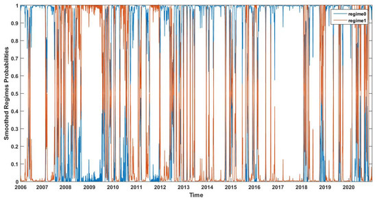
Figure 1.
Smoothed regime probabilities of the CRM-MRS model.
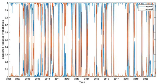
Figure 2.
Smoothed regime probabilities of the CRM-H-MRS model.
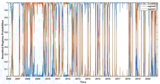
Figure 3.
Smoothed regime probabilities of the PM-MRS model.
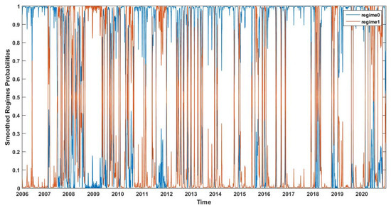
Figure 4.
Smoothed regime probabilities of the PM-H-MRS model.
5.2. In-Sample Volatility Prediction
In order to evaluate the volatility prediction performance of the interval regression models, we used the Parkinson variance estimator (Parkinson 1980) to transform the range prediction () into variance prediction:
The factor 1/(4ln(2)) derived by Parkinson (1980) is equal to the reciprocal of the second moment of the range of a standard Brownian motion when prices are observed continuously. This estimator is claimed to be five times more efficient than the traditional variance estimator based on daily returns. Then, we employed the following four common loss functions to evaluate the volatility forecasts:
where is the proxy for actual volatility at day t.9 It is clear that smaller loss function values correspond to better volatility forecasting performance.
Table 4 reports the average losses of the eight interval regression models, as well as the average losses of the point-data-based GARCH model10 and the range-based ECARR model. To assess the value of applying interval regression models for volatility forecasting, two-sided Diebold–Mariano (DM) tests (Diebold and Mariano 1995) were performed to compare each interval regression model with the point-data-based GARCH model. The numerical number marked with a “***” indicates that the corresponding DM test statistic is significant at the 1% level, with the interval regression model performing better. Besides, two-sided DM tests were also performed to compare each interval regression model with the commonly adopted ECARR model, which also utilizes daily range information. The numerical number marked with a “###” (“##”/“#”) indicates that the corresponding DM test statistic is significant at the 1% (5%/10%) level, with the interval regression model performing better. Furthermore, to evaluate the contribution of introducing the long memory HAR structure in the interval regression models, we performed a two-sided DM test to compare each long memory interval regression model with its corresponding short memory comparative. The number marked with a “†††” indicates that the corresponding DM test statistic is significant at the 1% level with the long memory model performing better. Last, to evaluate the contribution of introducing the nonlinear Markov regime switching structure in the interval regression models, we performed a two-sided DM test to compare each nonlinear interval regression model with its corresponding linear comparative. The number marked with a “‡‡‡” indicates that the corresponding DM test statistic is significant at the 1% level, with the nonlinear model performing better.
Table 4.
In-sample volatility prediction performance.
From Table 4 we can see that,
- (1)
- No matter which loss function is considered, all the eight interval regression models are marked with a “***”, which shows that these interval data-based models each provide significantly better in-sample volatility forecasts than the traditional point-data-based GARCH model.
- (2)
- No matter which loss function is considered, CRM-H, CRM-MRS, CRM-H-MRS, PM-H, PM-MRS, and PM-H-MRS are always marked with at least a “#”, which shows that these six models provide significantly better in-sample volatility forecasts than the range-based ECARR model. Considering the fact that the CRM class models and the ECARR model utilize similar range information and the basic CRM model is inferior to the ECARR model, we conclude that incorporating the HAR structure, the Markov regime switching structure, or both, can more effectively use the range information in terms of volatility forecasting.
- (3)
- No matter which loss function is considered, CRM-H, CRM-H-MRS, PM-H, and PM-H-MRS are always marked with a “†††”, which shows that these four models provide significantly better in-sample volatility forecasts than their short memory comparatives, thus further confirms the importance of characterizing the long memory property. This result validates the conclusion of Corsi (2009) and Andersen et al. (2007)—that the HAR framework is effective.
- (4)
- No matter which loss function is considered, CRM-MRS, CRM-H-MRS, PM-MRS, and PM-H-MRS are always marked with a “‡‡‡”, which shows that these models provide significantly better in-sample volatility forecasts than their linear comparatives, which further confirms the value of incorporating the Markov regime switching structure. This result is consistent with the results of Ma et al. (2017), Raggi and Bordignon (2012), and Shi and Ho (2015)—that incorporating Markov regime switching leads to fitting accuracy gains.
- (5)
- No matter which loss function is considered, the average losses of the PM class models are all smaller than those of the corresponding CRM class models. Besides, the best model is always the PM-H-MRS model, which indicates that the PM structure makes better use of interval information relative to the CRM structure. This result is reasonable, as Souza et al. (2017) points out that CRM is a particular case of PM.
To further pick out the best model, Table 5 reports p-values of the model confidence set (MCS) test (Hansen et al. 2011). The test can compare multiple models simultaneously without specifying the benchmark model and generate a confidence set containing one or more models which perform significantly better than the remaining models. At the significant level of 20%, the p-value being higher than 0.2 indicates the model is in the model confidence set . Table 5 shows that the PM-H-MRS model is the only model that survives in the confidence set in terms of all the four loss functions. This shows that incorporating both the HAR structure and the Markov regime switching structure in the PM model provides significantly superior in-sample volatility prediction.
Table 5.
In-sample MCS test p-values.
6. Out-of-Sample Results
In this section, we compared the prediction performance of the eight interval regression models, as well as the point-data-based GARCH model and the range-based ECARR model, in the out-of-sample forecast period from 4 January 2010 to 30 December 2020. The one-step-ahead rolling window forecast method was employed. Since the first 22 observations were used to calculate the monthly range on 6 February 2006, the first estimation window was from 6 February 2006 to 31 December 2009, altogether 984 days. This forecast period includes the European debt crisis from 2010 to 2011, China’s abnormal market fluctuations in 2015, the trade disputes between China and the United States in 2018, and the COVID-19 pandemic in 2020. To test the stability of the models under different market conditions, we used the nonparametric change point model (NPCPM) (Ross et al. 2011) to detect the volatility regimes of the S&P500 index during the out-of-sample forecast period and evaluate the models’ volatility prediction performance in different volatility regimes.
Figure 5 shows the volatility regimes detected by the NPCPM in the out-of-sample period from 4 January 2010 to 30 December 2020. There are seven volatility regimes. The first regime is from 4 January 2010 to 30 November 2011, altogether 482 trading days. We refer to it as the high volatility regime (H1 sub-period), since the S&P 500 index is volatile during this period. This regime corresponds to the European debt crisis from 2010 to 2011. The second regime is from 1 December 2011 to 20 August 2015, altogether 935 trading days. We refer to it as the low volatility regime (L sub-period), since the S&P 500 index is tranquil during this period. The third regime is from 21 August 2015 to 28 July 2016 (236 trading days). We refer to it as the high volatility regime (H2 sub-period) since the S&P500 index is also volatile during this period. This regime corresponds to China’s abnormal market fluctuations in 2015. Although both are high volatility regimes, the third regime is milder than the first regime. The fourth regime is from 29 July 2016 to 2 February 2018 (382 trading days). We again refer to it as the low volatility regime (L) since the S&P 500 index is extremely tranquil during this period. The fifth regime is from 5 February 2018 to 8 November 2019 (445 trading days). We refer to it as the high volatility regime (H3 sub-period) since the S&P500 index is extremely volatile during this period. This regime corresponds to the trade disputes between China and the United States in 2018. The sixth regime is from 11 November 2019 to 3 March 2020 (77 trading days), we refer to it as the low volatility regime (L) due to its similarity with the second and the fourth regimes. The last regime is from 4 March 2020 to 30 December 2020 (206 trading days), we refer to it as the high volatility regime (H4 sub-period) since the S&P500 index is also volatile during this period. This regime corresponds to the stock market shocks caused by the COVID-19 pandemic in 2020.
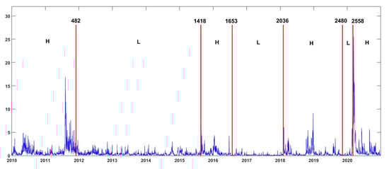
Figure 5.
Volatility regimes detected by the NPCPM in the out-of-sample period from 4 January 2010 to 30 December 2020 (S&P 500).
Table 6 reports the out-of-sample average losses of the eight interval regression models, the GARCH model and the ECARR model. Specifically, Panel A displays the results of the full out-of-sample period. Panel B displays the results of the first high volatility regime (H1 sub-period) from 4 January 2010 to 30 November 2011. Panel C displays the results of the second high volatility regime (H2 sub-period) from 21 August 2015 to 28 July 2016. Panel D displays the results of the third high volatility regime (H3 sub-period) from 5 February 2018 to 8 November 2019. Panel E displays the results of the fourth high volatility regime (H4 sub-period) from 4 March 2020 to 30 December 2020. Panel F displays the results of the three low volatility regimes (L sub-periods) from 1 December 2011 to 20 August 2015, from 29 July 2016 to 2 February 2018, and from 11 November 2019 to 3 March 2020. To assess the value of applying interval regression models for volatility forecasting, two-sided DM tests were performed to compare each interval regression model with the point-data-based GARCH model. “***” (“**”) indicates that the corresponding model significantly outperforms the GARCH model in the DM test at the 1% (5%) significance level. Besides, two-sided DM tests were also performed to compare each interval regression model with the commonly adopted ECARR model which also utilizes daily range information. The numerical number marked with a “###” (“##”/“#”) indicates that the corresponding model significantly outperforms the ECARR model at the 1% (5%/10%) significance level. Furthermore, to evaluate the contribution of introducing the long memory HAR structure in the interval regression models, we performed a two-sided DM test to compare each long memory interval regression model with its corresponding short memory comparative. “†††” (“††”/“†”) indicates that the corresponding model significantly outperforms its short memory comparative in the DM test at the 1% (5%/10%) significance level. Lastly, to evaluate the contribution of introducing the nonlinear Markov regime switching structure in the interval regression models, we performed a two-sided DM test to compare each nonlinear interval regression model with its corresponding linear comparative. “‡‡‡” (“‡‡”/“‡”) indicates that the corresponding model significantly outperforms its linear comparative in the DM test at the 1% (5%/10%) significance level.
Table 6.
Out-of-sample volatility prediction performance.
It can be seen from Table 6 that, in all the six panels, no matter which loss function is considered, all the eight interval regression models are marked with at least a “**”. This shows that the interval regression models each has significantly better volatility forecasting capability than the GARCH model, regardless of the market condition considered and the loss function specified, which is consistent with the in-sample fit results obtained in Table 4. This result is also consistent with the out-of-sample results in Fischer et al. (2016), illustrating the superiority of the interval regression models compared to the GARCH model.
Next, comparing the average losses of the CRM model, the CRM-MRS model, the PM model, and the PM-MRS model with the ECARR model shows that these four interval regression models outperform the ECARR model in the second, third, and fourth high volatility regimes (Panels C, D, and E), although the superiority is not significant. On the other hand, the CRM-H model, the CRM-H-MRS model, the PM-H model, and the PM-H-MRS model each effectively reduces the average losses relative to the ECARR model in all the six panels. Furthermore, their average losses are marked with at least a “#”, indicating that the superiority is significant. Thus, the CRM-H model, the CRM-H-MRS model, the PM-H model, and the PM-H-MRS model have significantly superior volatility forecasting accuracy over the ECARR model under all the market conditions, regardless of the loss function specified. Such an observation discloses that characterizing the long memory property through the HAR structure is valuable.
Third, the average losses of the CRM-H model, the CRM-H-MRS model, the PM-H model, and the PM-H-MRS model are all marked with at least a “†”, which indicates that incorporating the HAR structure significantly improves the prediction performance. This conclusion is robust under all the market conditions and all loss function specifications, which further confirms the value of characterizing the long memory property through the HAR structure.
Fourth, the PM-H-MRS model always has smaller average losses than the PM-H model. Meanwhile, the CRM-H-MRS model and the PM-MRS model outperform their linear comparatives in almost all the cases, respectively. This indicates that incorporating the Markov regime switching structure improves the predictive ability of the interval regression models, especially when our proposed PM framework is applied. This is consistent with the results of Ma et al. (2017) and Raggi and Bordignon (2012)—that incorporating Markov regime switching can improve out-of-sample volatility forecasting accuracy. Furthermore, the average losses of the PM-H-MRS model are all marked with at least a “‡”, which indicates that the superiority of the PM-H-MRS model over the PM-H model is significant under all the market conditions, regardless of the loss function specified. Therefore, under the proposed PM framework, the improvement from incorporating the Markov regime switching structure is significant when the heterogeneous structure is also characterized.
Last but not least, the PM-H-MRS model has the smallest average losses among all the ten models under all the market conditions. Based on this, we conclude that introducing the HAR structure together with the Markov regime switching structure in the PM framework leads to the significantly superior interval regression model in terms of volatility forecasting.
Table 7 reports the MCS test p-values for the out-of-sample period. A p-value greater than 0.2 indicates that the corresponding model is in the model confidence set and is significantly superior. We can see that the PM-H-MRS model has p-values of 1 in all the six forecast periods, regardless of the loss function specified, while the p-values of the other models are mostly less than 0.2, except for the CRM-H model and the CRM-H-MRS model in the H4 sub-period (from 4 March 2020 to 30 December 2020). Therefore, the PM-H-MRS model is significantly superior among all the ten models under all the market conditions. This is consistent with our observation from Table 6 and confirms the value of incorporating the long memory HAR structure, as well as the nonlinear Markov regime switching structure in the PM framework.
Table 7.
Out-of-sample MCS test p-values.
7. Discussion
In summary, empirical tests with the S&P 500 index daily price interval data show that: (1) the interval regression models each significantly improve the volatility prediction accuracy compared to the point-data-based GARCH model. (2) Incorporating the long memory HAR structure significantly improves the prediction accuracy and the long memory models significantly outperform the range-based ECARR model. (3) The two Markov regime switching PM class models each have superior volatility prediction performance over its linear comparative. In particular, this superiority is significant for the long memory PM-H-MRS model. (4) The PM-H-MRS model is significantly superior among all the interval regression models, including the classical CRM model and its long memory, nonlinear extensions. (5) The above conclusions are robust under all the market conditions, including the extremely volatile periods caused by the European debt crisis, China’s abnormal market fluctuations, the trade disputes between China and the United States, and the COVID-19 pandemic.
The above results are instructive for volatility prediction practice. Specifically, we summarize the following suggestions.
First, when high-frequency data are not available, interval regression models are preferred over the point-data-based GARCH model and the range-based ECARR model, and among the interval regression models, the PM model is suggested. Interval regression models can provide higher volatility prediction accuracy at low sampling cost. Second, while applying the interval regression models, it is important to incorporate the long memory HAR structure. Incorporating the HAR structure can significantly improve volatility prediction accuracy without complicating the parameter estimation procedure. Third, for those investors not restricted by technical complexity, the best volatility prediction choice is to use the PM-H-MRS model that further incorporates the Markov regime switching structure. Incorporating this nonlinear structure can significantly improve the volatility prediction accuracy of the PM class models at reasonable computation cost.
8. Conclusions and Outlook
Predicting volatility is critical for investors and risk managers. Considering the inferior volatility tracking capability of the point-data-based volatility models and the high data acquisition cost of the high-frequency data-based volatility models, we propose using daily price interval data and interval regression models for volatility prediction. Overall, the empirical comparisons in this research confirm the value of predicting volatility with interval regression models and disclose the importance of incorporating the long memory HAR structure, as well as the nonlinear Markov regime switching structure, in the interval regression models.
This paper sets the stage for future work in several directions. First, besides evaluating the statistical importance of forecasting volatility with interval regression models, scholars can also evaluate its economic importance under various application scenarios, e.g., option pricing and risk management. Second, based on our proposed interval regression models, one can introduce exogenous variables such as the VIX index, the investor attention index, and the investor sentiment index, etc., to further improve volatility forecasting accuracy. Last but not least, further work can consider the application of interval regression models in multi-asset volatility prediction practice.
Author Contributions
Data curation, M.H.; Formal analysis, M.H.; Funding acquisition, H.Q.; Investigation, H.Q.; Methodology, H.Q.; Project administration, H.Q.; Supervision, H.Q.; Writing—original draft, M.H.; Writing—review & editing, H.Q. All authors have read and agreed to the published version of the manuscript.
Funding
This research was funded by the National Natural Science Foundation of China [72171110 (Hui Qu)].
Data Availability Statement
The data that support the findings of this study are available from the corresponding author upon reasonable request.
Conflicts of Interest
The authors declare no conflict of interest.
Appendix A
In this appendix, we provide the in-sample (Table A1) and out-of-sample (Table A2) volatility prediction performance employing realized volatility (RV) as the proxy for actual volatility. Our purchased high-frequency data end on 15 May 2020. Thus, the last sub-period (H4 sub-period) in Table A2 is from 4 March 2020 to 15 May 2020 instead of from 4 March 2020 to 30 December 2020 as in Table 6.
The results are completely consistent with those employing as the proxy (Table 4 and Table 6), except during the H4 sub-period, when the PM-H model is superior to the PM-H-MRS model instead. This slight difference is understandable, since the H4 sub-period for Table A2 is much shorter due to data availability constraints.
Table A1.
In-sample volatility prediction performance employing RV as the proxy for actual volatility.
Table A1.
In-sample volatility prediction performance employing RV as the proxy for actual volatility.
| PM | PM-MRS | PM-H | PM-H-MRS | CRM | CRM-MRS | CRM-H | CRM-H-MRS | GARCH | ECARR | |
|---|---|---|---|---|---|---|---|---|---|---|
| MAE | 0.6211 *** | 0.5583 ***‡‡‡ | 0.4745 ***###††† | 0.4491 ***###†††‡‡‡ | 0.6260 *** | 0.5611 ***‡‡‡ | 0.5079 ***###††† | 0.4676 ***###†††‡‡‡ | 0.8569 | 0.5542 |
| MSE | 3.8894 *** | 3.9087 *** | 2.9392 ***###††† | 2.7847 ***###†††‡‡‡ | 3.9976 *** | 3.9960 ***‡ | 3.3186 ***###††† | 3.1888 ***###†††‡‡‡ | 4.8845 | 3.9152 |
| MAEln | 0.6403 *** | 0.5485 ***‡‡‡ | 0.4401 ***###††† | 0.4050 ***###†††‡‡‡ | 0.6461 *** | 0.5576 ***‡‡‡ | 0.4694 ***###††† | 0.4275 ***###†††‡‡‡ | 0.8282 | 0.5386 |
| MSEln | 0.6361 *** | 0.4728 ***‡‡‡ | 0.3141 ***###††† | 0.2619 ***###†††‡‡‡ | 0.6474 *** | 0.4857 ***‡‡‡ | 0.3514 ***###††† | 0.2886 ***###†††‡‡‡ | 1.0209 | 0.4636 |
Notes: Bolding means that the prediction performance is the best. “***” indicates that the corresponding model significantly outperforms the GARCH model in the DM test at the 1% significance level. “###” indicates that the corresponding model significantly outperforms the ECARR model in the DM test at the 1% significance level. “†††” indicates that the corresponding model significantly outperforms its short memory comparative in the DM test at the 1% significance level. “‡‡‡” (“‡”) indicates that the corresponding model significantly outperforms its linear comparative in the DM test at the 1% (10%) significance level.
Table A2.
Out-of-sample volatility prediction performance employing RV as the proxy for actual volatility.
Table A2.
Out-of-sample volatility prediction performance employing RV as the proxy for actual volatility.
| PM | PM-MRS | PM-H | PM-H-MRS | CRM | CRM-MRS | CRM-H | CRM-H-MRS | GARCH | ECARR | |
|---|---|---|---|---|---|---|---|---|---|---|
| Panel A: Full out-of-sample period. | ||||||||||
| MAE | 0.4542 *** | 0.4376 *** | 0.3896 ***###††† | 0.3248 ***###†††‡‡‡ | 0.4417 *** | 0.4477 *** | 0.3571 ***###††† | 0.3530 ***###†††‡ | 0.7133 | 0.4460 |
| MSE | 1.7055 *** | 1.6530 *** | 1.2876 ***##† | 1.0727 ***###†††‡‡ | 1.5703 *** | 1.7130 *** | 1.1830 ***##†† | 1.2146 ***###††† | 2.8588 | 1.8554 |
| MAEln | 0.6585 *** | 0.6346 *** | 0.5597 ***###††† | 0.4616 ***###†††‡‡‡ | 0.6405 *** | 0.6420 *** | 0.4871 ***###††† | 0.4890 ***#††† | 0.9227 | 0.6293 |
| MSEln | 0.6853 *** | 0.6216 ***‡ | 0.4978 ***###††† | 0.3478 ***###†††‡‡‡ | 0.6311 *** | 0.6313 *** | 0.3769 ***###††† | 0.3791 ***###††† | 1.2302 | 0.6367 |
| Panel B: H1 sub-period. | ||||||||||
| MAE | 0.7786 *** | 0.7590 *** | 0.6996 ***#††† | 0.5651 ***###†††‡‡‡ | 0.7836 *** | 0.7905 *** | 0.6289 ***##††† | 0.6245 ***###††† | 1.1403 | 0.7541 |
| MSE | 2.5712 *** | 2.0273 ***‡ | 2.2062 ***#† | 1.6450 ***###†††‡‡ | 2.2663 *** | 2.1755 *** | 2.0413 ***#†† | 1.9673 ***###††† | 3.9679 | 2.8114 |
| MAEln | 0.6379 *** | 0.6478 *** | 0.5474 ***#††† | 0.4431 ***###†††‡‡‡ | 0.6697 *** | 0.6660 *** | 0.4665 ***##††† | 0.4818 ***###††† | 0.8224 | 0.5871 |
| MSEln | 0.6451 *** | 0.6507 *** | 0.4707 ***###†† | 0.3209 ***###†††‡‡‡ | 0.6891 *** | 0.6803 *** | 0.3548 ***##††† | 0.3728 ***###††† | 0.9849 | 0.5625 |
| Panel C: H2 sub-period. | ||||||||||
| MAE | 0.6115 *** | 0.5819 *** | 0.5177 ***###††† | 0.4441 ***###†††‡‡‡ | 0.5906 *** | 0.6043 *** | 0.5101 ***###††† | 0.4967 ***###††† | 0.7883 | 0.6205 |
| MSE | 3.8096 *** | 3.6856 *** | 3.4946 ***##††† | 2.8792 ***###†††‡‡ | 3.7112 *** | 3.8202 *** | 3.3038 ***##††† | 3.2124 ***###††† | 4.2233 | 4.0737 |
| MAEln | 0.6513 *** | 0.5911 *** | 0.5104 ***###††† | 0.4302 ***###†††‡‡‡ | 0.6175 *** | 0.6257 *** | 0.4896 ***###††† | 0.4866 ***###††† | 0.8146 | 0.6487 |
| MSEln | 0.7200 *** | 0.6157 ***‡‡‡ | 0.4682 ***###††† | 0.3139 ***###†††‡‡‡ | 0.6375 *** | 0.6572 *** | 0.3968 ***###††† | 0.3855 ***###††† | 1.0545 | 0.7268 |
| Panel D: H3 sub-period. | ||||||||||
| MAE | 0.3628 *** | 0.3208 *** | 0.3258 ***###††† | 0.2473 ***###†††‡‡‡ | 0.3201 *** | 0.3221 *** | 0.2835 ***###††† | 0.2622 ***###††† | 0.6202 | 0.3840 |
| MSE | 0.5984 *** | 0.4115 *** | 0.4276 ***##††† | 0.2487 ***###†††‡‡‡ | 0.3931 *** | 0.4281 *** | 0.3266 ***###††† | 0.2998 ***###††† | 1.0264 | 0.6111 |
| MAEln | 0.6338 *** | 0.5850 *** | 0.5703 ***###††† | 0.4516 ***###†††‡‡‡ | 0.5820 *** | 0.5832 *** | 0.4775 ***###††† | 0.4603 ***###††† | 0.9377 | 0.6462 |
| MSEln | 0.6512 *** | 0.5536 ***‡‡ | 0.5056 ***###††† | 0.3147 ***###†††‡‡‡ | 0.5326 *** | 0.5435 *** | 0.3404 ***###††† | 0.3243 ***###††† | 1.2209 | 0.6635 |
| Panel E: H4 sub-period. | ||||||||||
| MAE | 2.8665 *** | 3.0472 *** | 2.2756 ***###††† | 2.1442 ***###††‡‡ | 2.7236 *** | 3.1251 *** | 2.2565 ***###††† | 2.3663 ***###††† | 6.2977 | 2.9261 |
| MSE | 29.971 *** | 35.8310 *** | 16.6850 ***###††† | 17.501 ***###††† | 29.659 *** | 36.921 *** | 16.6360 ***###††† | 19.654 ***###††† | 73.0520 | 34.2900 |
| MAEln | 0.6997 *** | 0.7011 *** | 0.5186 ***###††† | 0.5208 ***###††† | 0.6105 *** | 0.6894 *** | 0.4952 ***###††† | 0.5285 ***###††† | 1.1024 | 0.5779 |
| MSEln | 0.7348 *** | 0.7926 *** | 0.3789 ***###††† | 0.4322 ***###††† | 0.5964 *** | 0.7287 *** | 0.4076 ***###††† | 0.4376 ***###††† | 1.5677 | 0.5988 |
| Panel F: L sub-period. | ||||||||||
| MAE | 0.2600 *** | 0.2481 *** | 0.2148 ***###††† | 0.1825 ***###†††‡‡‡ | 0.2571 *** | 0.2490 *** | 0.1942 ***###††† | 0.1932 ***###†††‡ | 0.3877 | 0.2429 |
| MSE | 0.4178 | 0.3854 | 0.3330 ***###††† | 0.2591 ***###†††‡‡‡ | 0.3640 *** | 0.3801 ** | 0.2611 ***###††† | 0.2648 ***###††† | 0.3847 | 0.4158 |
| MAEln | 0.6733 *** | 0.6509 *** | 0.5703 ***###††† | 0.4745 ***###†††‡‡‡ | 0.6540 *** | 0.6536 *** | 0.4966 ***###††† | 0.4997 ***###††† | 0.9648 | 0.6370 |
| MSEln | 0.7026 *** | 0.6282 *** | 0.5139 ***###††† | 0.3706 ***###†††‡‡‡ | 0.6426 *** | 0.6345 *** | 0.3919 ***###††† | 0.3958 ***###††† | 1.3365 | 0.6399 |
Notes: Panel A displays the results of the full out-of-sample period. Panel B displays the results of the first high volatility regime (H1 sub-period) from 4 January 2010 to 30 November 2011. Panel C displays the results of the second high volatility regime (H2 sub-period) from 21 August 2015 to 28 July 2016. Panel D displays the results of the third high volatility regime (H3 sub-period) from 5 February 2018 to 8 November 2019. Panel E displays the results of the fourth high volatility regime (H4 sub-period) from 4 March 2020 to 15 May 2020. Panel F displays the results of the three low volatility regimes (L sub-periods) from 1 December 2011 to 20 August 2015, from 29 July 2016 to 2 February 2018 and from 11 November 2019 to 3 March 2020. Bolding means that the prediction performance is the best. “***” (“**”) indicates that the corresponding model significantly outperforms the GARCH model in the DM test at the 1% (5%) significance level. “###” (“##”/“#”) indicates that the corresponding model significantly outperforms the ECARR model in the DM test at the 1% (5%/10%) significance level. “†††” (“††”/“†”) indicates that the corresponding model significantly outperforms its short memory comparative in the DM test at the 1% (5%/10%) significance level. “‡‡‡” (“‡‡”/“‡”) indicates that the corresponding model significantly outperforms its linear comparative in the DM test at the 1% (5%/10%) significance level.
Notes
| 1 | The volatility forecasting performance gains from modeling the range based estimators have been demonstrated in numerous studies (Chou 2005; Chou et al. 2009; Brownlees and Gallo 2010), which confirm the merits of employing the daily price interval information to some extent. The most commonly used range model is the conditional autoregressive range (CARR) model with the disturbance term assumed to follow the exponential distribution with a unit mean (ECARR). |
| 2 | We also extended the CRM model by incorporating the HAR structure and the Markov regime switching structure in order to better analyze the advantages of the long memory and nonlinear extensions. The corresponding models are referred to as the CRM-H model, the CRM-MRS model, and the CRM-H-MRS model, respectively. |
| 3 | The predicted ranges are not negative for both the CRM model and the CRM-H model in our empirical experiments. |
| 4 | In order to guarantee the non-negativity of the predicted interval range, Souza et al. (2017) suggest using the Box-Cox transformation for the response variable. Our empirical results show that the predicted ranges are not negative even without the Box-Cox transformation. |
| 5 | In empirical applications of the Markov regime switching structure, two regimes are usually assumed; see Raggi and Bordignon (2012), Shi and Ho (2015) and Wang et al. (2016) for examples. |
| 6 | This paper is an instrumental article providing Matlab code and its descriptions. The detailed estimation procedure and forecasting procedure can be found in pages 7 to 9 in Perlin (2015). |
| 7 | Price data were amplified by a factor of 100. |
| 8 | A trader mistyped millions (m) as billions (b) while selling a stock, causing a sudden intraday plunge of the stock market. |
| 9 | We also used realized volatility calculated as the sum of squared intraday 10-minute logarithmic returns (Andersen and Bollerslev 1998) as the proxy for actual volatility. The high-frequency data were collected from PiTrading and span from 3 January 2006 to 15 May 2020. The corresponding results can be found in Appendix A, which hardly change the in-sample and out-of-sample conclusions. |
| 10 | The GARCH (1,1) specification was selected according to the AIC and BIC rules. |
References
- Andersen, Torben G., and Tim Bollerslev. 1998. Answering the skeptics: Yes, standard volatility models do provide accurate forecasts. International Economic Review 39: 885–905. [Google Scholar] [CrossRef]
- Andersen, Torben G., Tim Bollerslev, and Francis X. Diebold. 2007. Roughing it up: Including jump components in the measurement, modeling, and forecasting of return volatility. The Review of Economics and Statistics 89: 701–20. [Google Scholar] [CrossRef]
- Barndorff-Nielsen, Ole E., Peter Reinhard Hansen, Asger Lunde, and Neil Shephard. 2008. Designing realized kernels to measure the ex post variation of equity prices in the presence of noise. Social Science Electronic Publishing 76: 1481–536. [Google Scholar]
- Billard, Lynne, and Edwin Diday. 2000. Regression Analysis for Interval-Valued Data. Data Analysis, Classification, and Related Methods. Berlin/Heidelberg: Springer, pp. 369–74. [Google Scholar]
- Billard, Lynne, and Edwin Diday. 2002. Symbolic regression analysis. Studies in Classification Data Analysis & Knowledge Organization 37: 6317–28. [Google Scholar]
- Bollerslev, Tim. 1986. Generalized autoregressive conditional heteroskedasticity. Journal of Econometrics 31: 307–27. [Google Scholar] [CrossRef]
- Brownlees, Christian T., and Giampiero M. Gallo. 2010. Comparison of volatility measures: A risk management perspective. Journal of Financial Econometrics 8: 29–56. [Google Scholar] [CrossRef]
- Chou, Ray Yeutien. 2005. Forecasting financial volatilities with extreme values: The conditional autoregressive range (CARR) model. Journal of Money, Credit and Banking 37: 561–82. [Google Scholar] [CrossRef]
- Chou, Ray Yeutien, Chun-Chou Wu, and Nathan Liu. 2009. Forecasting time-varying covariance with a range-based dynamic conditional correlation model. Review of Quantitative Finance & Accounting 33: 327–45. [Google Scholar]
- Corsi, Fulvio. 2009. A simple approximate long-memory model of realized volatility. Journal of Financial Econometrics 7: 174–96. [Google Scholar] [CrossRef]
- Diebold, Francis, and Robert Mariano. 1995. Comparing predictive accuracy. Journal of Business & Economic Statistics 13: 253–63. [Google Scholar]
- Fischer, Henning, Ángela Blanco-Fernández, and Peter Winker. 2016. Predicting stock return volatility: Can we benefit from regression models for return intervals? Journal of Forecasting 35: 113–46. [Google Scholar]
- González-Rivera, Gloria, and Wei Lin. 2013. Constrained regression for interval-valued data. Journal of Business & Economic Statistics 31: 473–90. [Google Scholar]
- Hamilton, James D. 1989. A new approach to the economic analysis of nonstationary time series and the business cycle. Econometrica 57: 357–84. [Google Scholar] [CrossRef]
- Hansen, Peter R., Asger Lunde, and James M. Nason. 2011. The model confidence set. Econometrica 79: 453–97. [Google Scholar] [CrossRef]
- Klaassen, Franc. 2002. Improving Garch volatility forecasts with regime-switching Garch. Empirical Economics 27: 363–94. [Google Scholar] [CrossRef]
- Lima Neto, Eufrásio A., and Francisco de A. T. De Carvalho. 2008. Centre and range method to fitting a linear regression model on symbolic interval data. Computational Statistics & Data Analysis 52: 1500–15. [Google Scholar]
- Lima Neto, Eufrásio A., and Francisco de A. T. De Carvalho. 2010. Constrained linear regression models for symbolic interval-valued variables. Computational Statistics & Data Analysis 54: 333–47. [Google Scholar]
- Ma, Feng, Mohamed Ismail M. Wahab, Dengshi Huang, and Weiju Xu. 2017. Forecasting the realized volatility of the oil futures market: A regime switching approach. Energy Economics 67: 136–45. [Google Scholar] [CrossRef]
- Mincer, Jacob A., and Victor Zarnowitz. 1969. The evaluation of economic forecasts. In Economic Forecasts and Expectations: Analysis of Forecasting Behavior and Performance. Cambridge: NBER, pp. 3–46. [Google Scholar]
- Parkinson, Michael. 1980. The extreme value method for estimating the variance of the rate of return. The Journal of Business 53: 61–65. [Google Scholar] [CrossRef]
- Perlin, Marcelo. 2015. MS_Regress—The Matlab Package for Markov Regime Switching Models. Available online: https://ssrn.com/abstract=1714016 (accessed on 20 October 2022).
- Raggi, Davide, and Silvano Bordignon. 2012. Long memory and nonlinearities in realized volatility: A markov switching approach. Computational Statistics & Data Analysis 56: 3730–42. [Google Scholar]
- Ross, Gordon J., Dimitris K. Tasoulis, and Niall M. Adams. 2011. Nonparametric monitoring of data streams for changes in location and scale. Technometrics 53: 379–89. [Google Scholar] [CrossRef]
- Shi, Yanlin, and Kin-Yip Ho. 2015. Long memory and regime switching: A simulation study on the Markov regime-switching ARFIMA model. Journal of Banking & Finance 61: 189–204. [Google Scholar]
- Souza, Leandro C., Renata M. C. R. Souza, Getúlio J. A. Amaral, and Telmo M. Silva Filho. 2017. A parametrized approach for linear regression of interval data. Knowledge-Based Systems 131: 149–59. [Google Scholar] [CrossRef]
- Sun, Yuying, Ai Han, Yongmiao Hong, and Shouyang Wang. 2018. Threshold autoregressive models for interval-valued time series data. Journal of Econometrics 206: 414–46. [Google Scholar] [CrossRef]
- Taylor, Stephen John. 1982. Financial returns modelled by the product of two stochastic processes-a study of the daily sugar prices 1961–75. Time Series Analysis: Theory and Practice 1: 203–26. [Google Scholar]
- Wang, Yudong, Feng Ma, Yu Wei, and Chongfeng Wu. 2016. Forecasting realized volatility in a changing world: A dynamic model averaging approach. Journal of Banking & Finance 64: 136–49. [Google Scholar]


Publisher’s Note: MDPI stays neutral with regard to jurisdictional claims in published maps and institutional affiliations. |
© 2022 by the authors. Licensee MDPI, Basel, Switzerland. This article is an open access article distributed under the terms and conditions of the Creative Commons Attribution (CC BY) license (https://creativecommons.org/licenses/by/4.0/).