Abstract
In some applications of supervised machine learning, it is desirable to trade model complexity with greater interpretability for some covariates while letting other covariates remain a “black box”. An important example is hedonic property valuation modeling, where machine learning techniques typically improve predictive accuracy, but are too opaque for some practical applications that require greater interpretability. This problem can be resolved by certain structured additive regression (STAR) models, which are a rich class of regression models that include the generalized linear model (GLM) and the generalized additive model (GAM). Typically, STAR models are fitted by penalized least-squares approaches. We explain how one can benefit from the excellent predictive capabilities of two advanced machine learning techniques: deep learning and gradient boosting. Furthermore, we show how STAR models can be used for supervised dimension reduction and explain under what circumstances their covariate effects can be described in a transparent way. We apply the methodology to residential land and structure valuation, with very encouraging results regarding both interpretability and predictive performance.
1. Introduction
Machine learning (ML) techniques—such as artificial neural networks, random forests, and gradient boosting—can be more accurate than standard approaches—such as ordinary least squares—because they automatically learn relevant nonlinearities, transformations, and high-order interactions among the independent variables. These modeling techniques are increasingly being applied to house price modeling. Examples include Worzala et al. (1995), Din et al. (2001), and Zurada et al. (2011) for neural networks, Yoo et al. (2012) for random forests, Kagie and Wezel (2007) and Sangani et al. (2017) for boosting, and many contributions to the machine learning competition platform kaggle.com. Machine learning techniques generally yield more accurate predictions than standard linear models.
While ML techniques can be powerful predictive tools, they are often considered black boxes due to their limited interpretability (Din et al. 2001; Mayer et al. 2019). In some applications, this is particularly problematic due to a need for transparency in describing the effects of certain covariates. For example, in the case of hedonic modeling of house prices, it is desirable to identify the effects of some features, while others do not require individual interpretation. Specifically, there is often a need to explicitly measure the effects of structural (or building) characteristics, while locational attributes can be considered as a group. This is the case, for example, when appraising properties for taxation or mortgage underwriting purposes. Moreover, there is typically collinearity among locational attributes, making it difficult to identify their separate effects in any case. This paper demonstrates machine learning techniques with restricted complexity that allow for transparency with respect to a subset of the covariates while also achieving excellent predictive results. We apply the methods to house price valuation in South Florida and Switzerland. We believe that this is the first application of these techniques to the problem of real estate valuation.
The model structure considered in this article is described in Hothorn et al. (2010). There, a distributional property of a response variable Y is represented as a function f of input features in the structured form
where each additive component uses a subset of the q covariates. Such models can be viewed as a generalization of structured additive regression (STAR) models; see, e.g., Chapter 9 in Fahrmeir et al. (2013). Throughout this article, for the sake of simplicity, we also call them STAR models.
Important special cases of (1) are the generalized linear model (GLM, Nelder and Wedderburn 1972):
and the generalized additive model (GAM) without interactions (Hastie and Tibshirani 1986, 1990; Wood 2017)
The property is implied by specifying a loss function relevant to the problem at hand. Important examples are the squared error loss (), the absolute error loss (), and the log loss associated with the negative log-likelihood of the Bernoulli distribution ().
Having access to training data with optional case weights , the task to estimate with functions amounts to minimizing the average weighted loss over the training data, i.e., solving the task
subject to algorithmic constraints; see Hothorn et al. (2010) for details.
Different algorithms exist for solving the optimization task (3), each with its own characteristics and limitations. Traditional options include penalized iteratively reweighted least squares (Wood 2017), Bayesian optimization (Umlauf et al. 2012), and model-based gradient boosting or “mboost” (Bühlmann and Hothorn 2007). The latter uses component-wise gradient boosting, where each component represents a base learner chosen from a rich set of possibilities, including (penalized) least squares for linear effects and fixed or random categorical effects, (penalized) B-splines for smooth effects and two-dimensional interaction surfaces, and decision trees for representing the effects of any number of features. During each gradient update, the component with the best loss improvement is multiplied by the specified learning rate and added to the current prediction function. The algorithm “mboost” is implemented in the R package mboost; see, again, Hothorn et al. (2010).
In the next section, we show how STAR models in the form of (1) can also be fitted with deep learning, as well as with the high-performance gradient boosting implementations of XGBoost (Chen and Guestrin 2016) and LightGBM (Ke et al. 2017). Additionally, we discuss the possibility of using STAR models for supervised dimension reduction, e.g., to compress the information represented by a large set of locational features, and we explain under what circumstances feature effects can be transparently described, including the effects of certain multivariate components. The following two sections apply these ideas to the data from Florida and Switzerland, respectively. A final section discusses our conclusions.
2. Methodology
2.1. STAR Models and Deep Learning
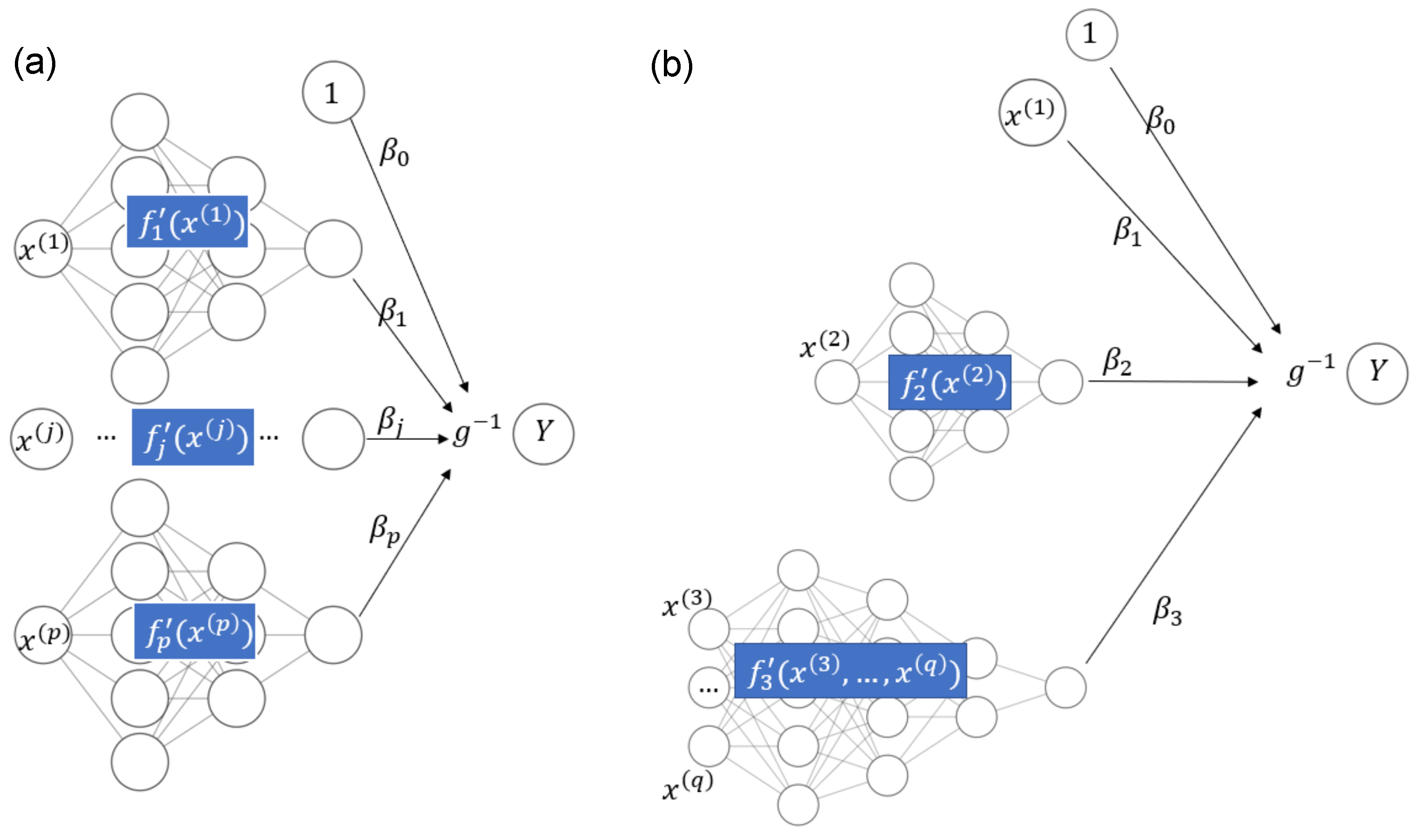
Recently, owing to the flexibility of implementations such as TensorFlow (see Abadi et al. 2016), deep learning approaches can also be used for fitting STAR models. In Agarwal et al. (2021), neural additive models are discussed. Such models use sub-networks to represent each input variable with a smooth function and connect their output nodes directly to the response Y, which is possibly transformed by a non-linear activation function ; see Figure 1a for an illustration. A neural additive model thus allows the fitting of additive models of the form
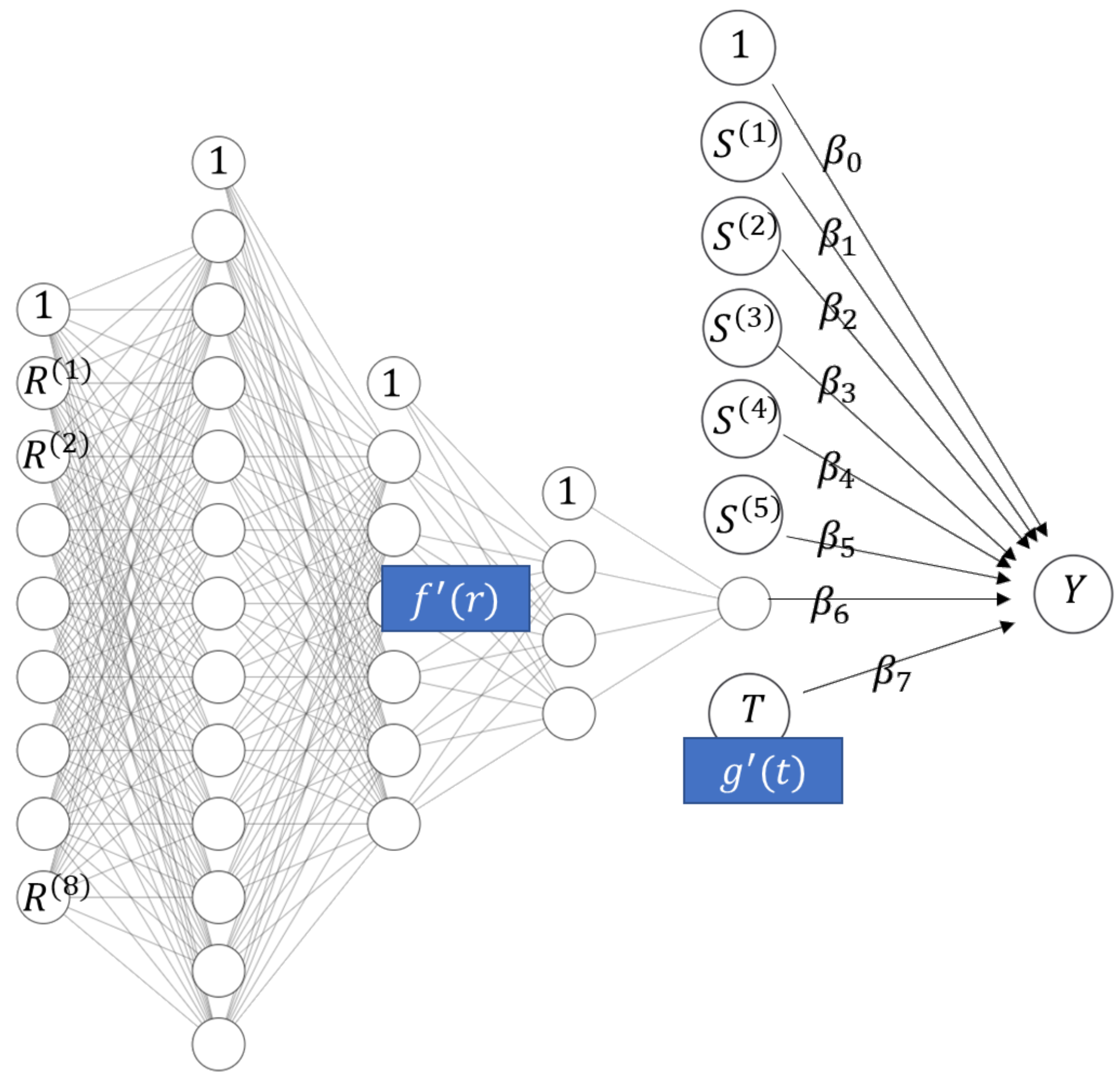
in line with (2). To fit a STAR model in the general case of (1) through deep learning, we need to slightly generalize the structure of the neural additive model to allow the sub-networks to use as input all covariates used in component ; see Figure 1b for a schematic example with the equation
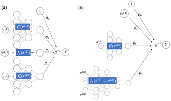
Figure 1.
(a) Neural additive model. (b) STAR model with one linear component, one smooth component of a single covariate, and one smooth component of multiple covariates.
Related models are discussed in Rügamer et al. (2021) in an even more general context of multivariate , allowing for modeling of the full conditional distribution of Y.
2.2. STAR Models and Gradient Boosting
Tree-based gradient boosting machines (Friedman 2001) belong to the best performing ML algorithms for tabular data, and major implementations, such as XGBoost (Chen and Guestrin 2016), LightGBM (Ke et al. 2017), and CatBoost (Prokhorenkova et al. 2018), dominate corresponding ML competitions (see Arik and Pfister 2019). It is well known that such models can be used to learn additive models of the form (2) by using tree stumps (trees with a single split) as base learners; see Lou et al. (2012) or Nori et al. (2019). Allowing more splits in the trees would introduce interaction effects, leading to non-additive models.
However, it is less known that some modern implementations of gradient boosting are actually able to non-parametrically fit STAR models of the form (1). The solution is based on imposing so-called feature interaction constraints, an idea that goes back to Lee et al. (2015). Their approach was implemented in 2018 in XGBoost, and, on our request, (Mayer 2020) in LightGBM in 2020 as well. Interaction constraints are specified as a collection of feature subsets , where each specifies a group of features that are allowed to interact. Algorithmically, the constraints are enforced by the following simple rule during tree growth: At each split, the set of split candidates is the union of those that contain all previously used split variables of the current branch.
Consequently, each tree branch uses features from one feature set only. Its associated prediction on the scale of contributes to the component of an implicitly defined STAR model of the form (1), where each model component uses feature subset as specified by the constraints.
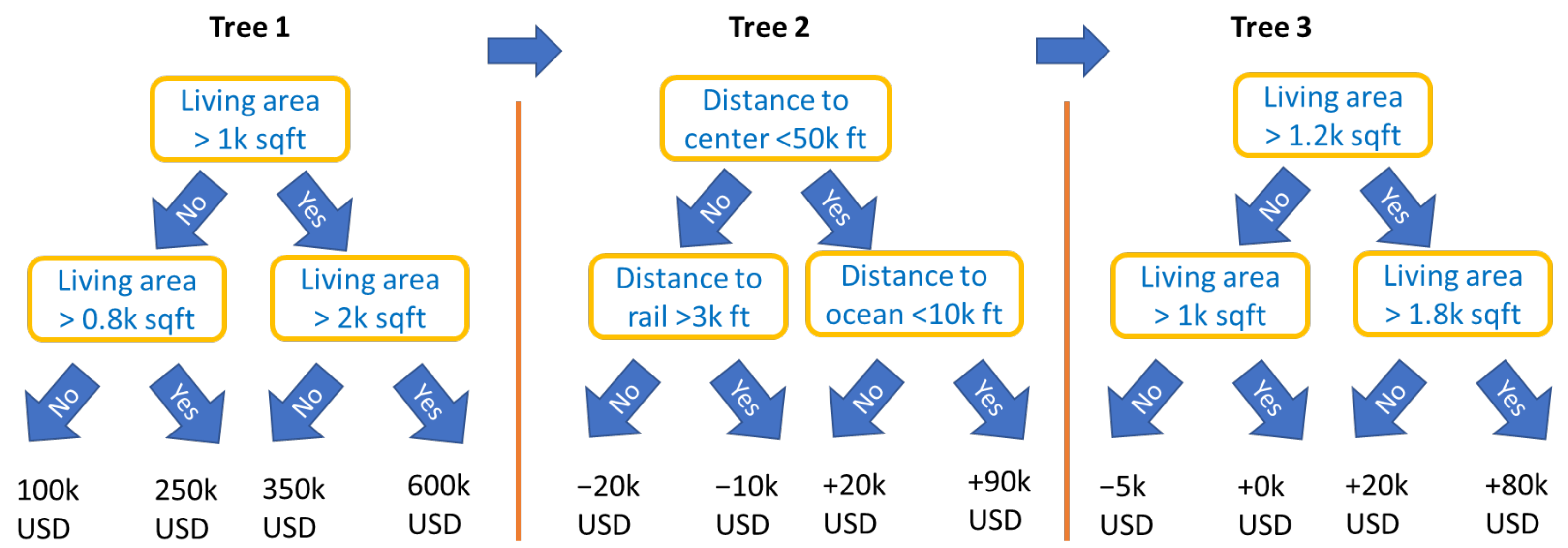
An important type of constraint is feature partitions, i.e., disjoint feature sets . They include the special case of the collection of singletons that would produce an additive model of the form (2). For partitions, by the above rule, the first split variable of a tree determines the feature set to be used throughout that tree. Figure 2 illustrates a simple example of such a model with the following equation:
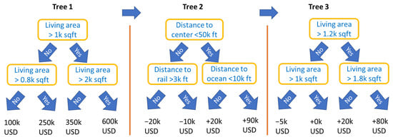
Figure 2.
Schematic view of three boosted trees with interaction constraints, representing a STAR model being additive in a living area and in a group of locational variables.
The corresponding constraints form a feature partition specified by
In the two programming languages R and Python, interaction constraints for XGBoost and LightGBM are specified as part of the parameter list passed to the corresponding train method. Table 1 shows how to specify the interaction_constraints parameter for an example with covariates A, B, C, and D and interaction constraints and corresponding to a model as in Figure 2.

Table 1.
Specifying the interaction_constraints parameter.
XGBoost and LightGBM offer different loss/objective functions. These specify the functional to be modeled; see Table 2 for some of the possibilities.
Table 2.
Important losses and functionals and how their corresponding objectives are specified in XGBoost and LightGBM.
Remark 1.
- At the time of writing and until at least XGBoost version 1.4.1.1, XGBoost respects only non-overlapping interaction constraint sets , i.e., partitions. LightGBM can also deal with overlapping constraint sets.
- Boosted trees with interaction constraints support only non-linear components, unlike, e.g., deep learning and component-wise boosting, both of which allow a mix of linear and non-linear components. See Remark 4, as well as our two case studies, for a two-step procedure that would linearize some effects fitted by XGBoost or LightGBM, thus overcoming this limitation.
- Feature pre-processing for boosted trees is simpler than for other modeling techniques. Missing values are allowed for most implementations, feature outliers are unproblematic, and some implementations (including LightGBM) can directly deal with unordered categorical variables. Furthermore, highly correlated features are only problematic for interpretation, not for model fitting.
- Model-based boosting “mboost” with trees as building blocks is an alternative to using XGBoost or LightGBM with interaction constraints.
2.3. STAR Models and Supervised Dimension Reduction
Since STAR models (including GAMs with two-dimensional interaction surfaces) typically use only a small subset of (interacting) features per component, the keyword “dimension reduction” rarely appears in connection with this type of model. However, a strength of tree-based components (e.g., trees as base learners in model-based boosting “mboost” or the approach via interaction constraints) and deep learning is that some components can use even a large number of interacting features. Such components serve as one-dimensional representations of their features, conditional on the other features. The values of such components (or sometimes of sums of multiple components) might be used as derived features in another model or analysis. Thus, STAR models offer an effective way to perform (one-dimensional) supervised dimension reduction. Note that, by supervised, we mean that the dimension reduction procedure uses the response variable of the model. Some examples illustrate this.
Example 1.
- 1.
- House price models with additive effects for structural characteristics and time (for maximal interpretability) and one multivariate component using all locational variables with complex interactions (for maximal predictive performance). The model equation could be as follows:Component provides a one-dimensional representation of all locational variables. We will see an example of such a model in the Florida case study.
- 2.
- This is similar to the first example, but adding the date of sale to the component with all locational variables, leading to a model with time-dependent location effects. The component depending on locational variables and time represents those variables by a one-dimensional function. Such a model will be shown in the Swiss case study below.
In the above examples, the feature subsets used by components are non-overlapping, i.e., are partitions. For a STAR model f of the general form (1), where features might appear in multiple components, we can extend the above idea of dimensionality reduction.
Definition 1 (Purely additive contributions and encoders).
Let be a feature subset of interest and the fitted additive components of a STAR model
as in Equation (1). The contribution of to the predictor is given by the partial predictor
where denotes the index set of components using features in . Furthermore, we call a purely additive contribution or encoder of if , i.e., if depends solely on features in . In this case, we say that has a purely additive contribution or is encodable and write the encoder as , where are values of the feature vector corresponding to .
Remark 2.
- From the above definition, it directly follows that the purely additive contribution of a (possibly large) set of features provides a supervised one-dimensional representation of the features in , optimized for predictions on the scale of ξ and conditional on the effects of other features.
- For simplicity, we assume that each model component is irreducible, i.e., it uses only as many features as necessary. In particular, a component additive in its features would be represented by multiple components instead.
- The encoder of is defined up to a shift, i.e., for any constant c is an encoder of as well. If c is chosen so that the average value of the encoder is 0 on some reference dataset, e.g., the training dataset, we speak of a centered encoder.
Example 2.
Consider the fitted STAR model
Following the above definition, we can say:
- 1.
- Let . Then,is a purely additive contribution of .
- 2.
- Due to interaction effects, the singleton and are not encodable.
- 3.
- Let and . Then,is an encoder of .
- 4.
- The fitted model is an encoder of the set of all features. This is true for STAR models in general.
Next, we consider the fitted STAR model
Here, the feature sets and form a partition. As a direct consequence of Definition 1, each feature set (and all its possible unions) of a partition is encodable. This property will implicitly be used in both of our case studies.
Depending on the implementation of the STAR algorithm, it might be possible to directly extract the encoder of a feature set from the fitted model. A procedure that works independently of the implementation is described in the following Algorithm 1, which requires only access to the prediction function on the scale of .
| Algorithm 1 Encoder extraction |
|
Remark 3 (Raw scores and boosting).
By default, predictions of XGBoost and LightGBM are on the scale of Y. If the functional ξ includes a link function (e.g., log or logit), one can obtain predictions on the scale of ξ via the argument outputmargin (XGBoost) or rawscore (LightGBM) of their predict method. This is relevant for the application of Algorithm 1 and also for interpretation of effects, as in Section 2.4.
The values of a (possibly centered) encoder of a feature set can be used as a one-dimensional representation of for subsequent analyses, e.g., as a derived covariate in a simplified regression model. In the case studies below, we will see that this approach produces models with an excellent trade-off between interpretability and predictive strength.
Example 3.
For instance, after fitting the STAR model (4) of Example 1 with XGBoost, we could extract the (centered) purely additive contribution of all location covariates using Algorithm 1 and calculate a subsequent linear regression of the form
where represent the values of the locational variables. The main difference with the initial XGBoost model is that the effects of the building characteristics are now linear.
Remark 4 (Modeling strategy).
The workflow in the last example is in line with the following general modeling strategy. Groups of related features (for instance, a large set of locational variables) are sometimes difficult to represent in a linear regression model. How should the features be transformed? What interactions are important? How should one deal with strong multicollinearity? These burdens could be delegated to an initial STAR model of suitable structure. Then, the model components representing such feature groups would be extracted and plugged as high-level features into a subsequent linear regression model. This allows one, e.g., to linearize some additive effects of a fitted boosted trees model with interaction constraints.
Encoders are also helpful for interpreting effects in general STAR models, as will be explained in the next section.
2.4. Interpreting STAR Models
In this section, we provide some information on how to interpret effects of features and feature sets in general STAR models (1), with a special focus on simple, fully transparent descriptions. These techniques will be used later in the case studies.
One of the most common techniques to describe the effect of a feature set in an ML model is the partial dependence plot (PDP) introduced in Friedman (2001). It visualizes the average partial effect of by taking the average of many individual conditional expectation profiles (ICE, see Goldstein et al. 2015). The ICE profile for the ith observation with observed covariate vector and feature set is calculated by evaluating predictions over a sufficiently fine grid of values for vector components corresponding to , keeping all other vector components of fixed. The stronger the interaction effects from other features, the less parallel the ICE profiles across multiple observations are. Thus, a visual test for additivity can be performed by plotting many ICE profiles and checking if they are parallel (see Goldstein et al. 2015). Conversely, if all ICE profiles of are parallel, is represented by the model in an additive way. In that case, a single ICE profile (or the PDP) serves as a fully transparent description of the effect of in the sense that it is clear how acts on globally for all observations ceteris paribus.
Studying ICE and PDP plots is not only interesting for interpreting feature effects in complex ML models. Along with other general-purpose tools from the field of explainable ML (see, e.g., Biecek and Burzykowski 2021; Molnar 2019), they can also be used to interpret models of restricted complexity, such as linear regression models, GAMs, or STAR models. There, they serve as (feature-centric) alternatives to partial residual plots (Wood 2017) that are frequently used to visualize effects of single model components. Note that, up to a vertical shift, partial residual plots coincide with ICE curves for features that appear in only one (single-feature) component.
In the context of STAR models, from Definition 1, it is easy to see that, for a feature set that has a purely additive contribution, ICE profiles of are parallel across all observations, and their values correspond to values of the encoder evaluated over the domain of (up to an additive constant). This includes centered or uncentered encoders as extracted by Algorithm 1. In fact, Algorithm 1 differs from the calculation of ICE profiles only in terms of technical details.
Thus, the effects of an encodable feature set can be described in a simple yet transparent way by, e.g., showing one ICE profile, the PDP, or by evaluating its encoder over the domain of . This is a major advantage of STAR models over unstructured ML models, where transparent descriptions of feature effects are unrealistic due to complex high-order interactions.
However, since it is difficult to describe ICE/PDP/encoders of more than two features, this concept is limited from a practical perspective to feature sets with only one or two features.
Remark 5.
- To benefit from additivity, effects of features in STAR models are typically interpreted on the scale of ξ.
- ICE profiles and the PDP can be used to interpret effects of non-encodable feature sets as well. Due to interaction effects, however, a single ICE profile or a PDP cannot give a complete picture of such an effect.
- In this paper, we describe feature effects by ICE/PDP/encoders. For alternatives, see Molnar (2019) or Biecek and Burzykowski (2021).
We have mentioned that describing multivariable ICE/PDP/encoders of more than two features is difficult in practice. However, depending on the modeling situation, it is not uncommon that a possibly large, encodable feature set represents a low-dimensional feature set with mapping . Here, and denote feature vectors corresponding to feature sets and . In this case, the ICE/PDP/encoder can be evaluated over values of to provide, again, a fully transparent description of the effects of and . Thus, instead of using the encoder with high-dimensional , we would use the equivalent encoder with low-dimensional to describe the effects of feature set (or ), even if we cannot exactly describe the effects of single features in .
We have seen three such situations in Example 1: The full set of location variables can represent low-dimensional features, such as:
- The administrative unit (a one-dimensional feature).
- The address (also a one-dimensional feature).
- Latitude/longitude (a two-dimensional feature).
Similarly, time-dependent location effects could represent the two features “administrative unit” and “time”.
3. Case Study 1: Miami Housing Data
To apply the above methods, we consider two case studies involving hedonic house price models. Hedonic models are widely used in the context of real estate valuation, especially for residential properties (Malpezzi 2003). Such models apply information about a sample of properties that transacted to estimate models that are then used to predict the values of out-of-sample properties that did not transact. The dependent variable is the price of the properties and the independent variables are a set of physical and locational attributes. Hedonic models are a valuable tool for property tax appraisers, mortgage underwriters, valuation firms, and regulatory authorities. Popular online resources, such as Zillow.com in the United States, rely on such models to provide regularly updated estimates of property values. Various studies have successfully applied machine learning techniques to hedonic models (e.g., Mayer et al. 2019; Wei et al. 2022), but interpretability remains an issue.
3.1. Data
This case study uses information on 13,932 single-family homes sold at arm’s length in Miami in 2016. The data are collected by county property tax appraisers and distributed for research purposes by the Florida Department of Revenue. Aside from sale price and time, the dataset contains five building characteristics and eight locational variables; see Table 3 for definitions of the variables and Figure 3, Figure 4, Figure 5 and Figure 6 for a descriptive analysis.
Table 3.
Variables used in the Miami case study.

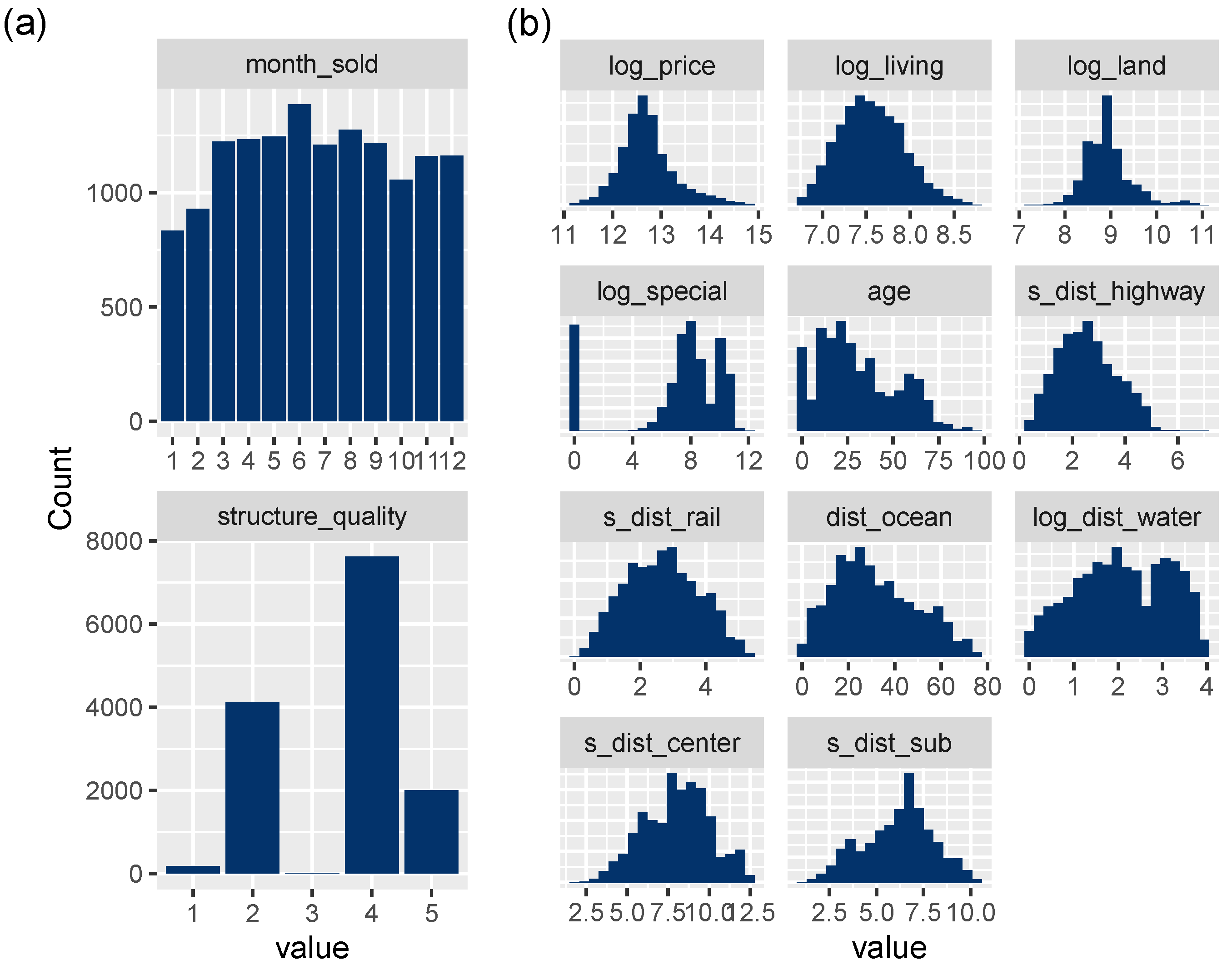
Figure 3.
(a) Bar plots of discrete variables. (b) Histograms of transformed continuous variables, except latitude/longitude.

Figure 4.
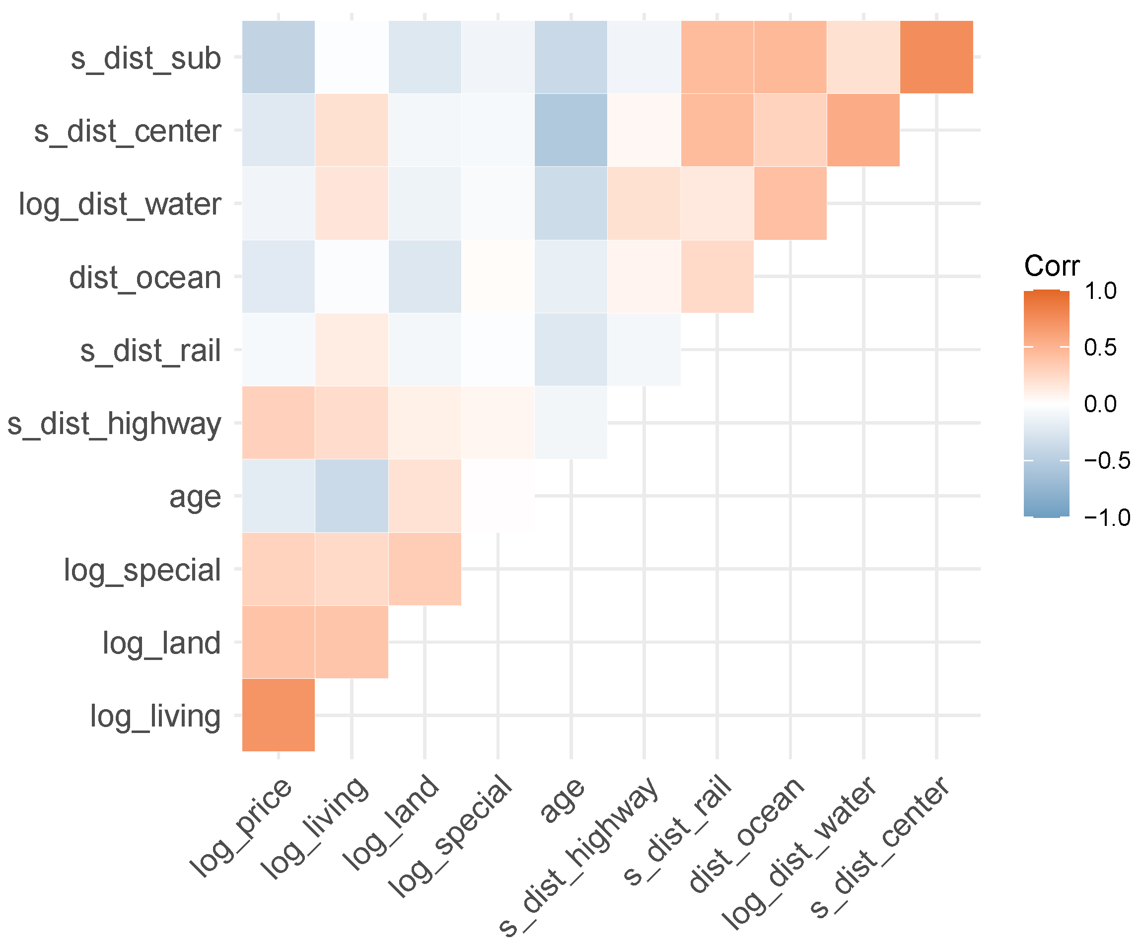
Correlogram of continuous variables (except latitude/longitude).

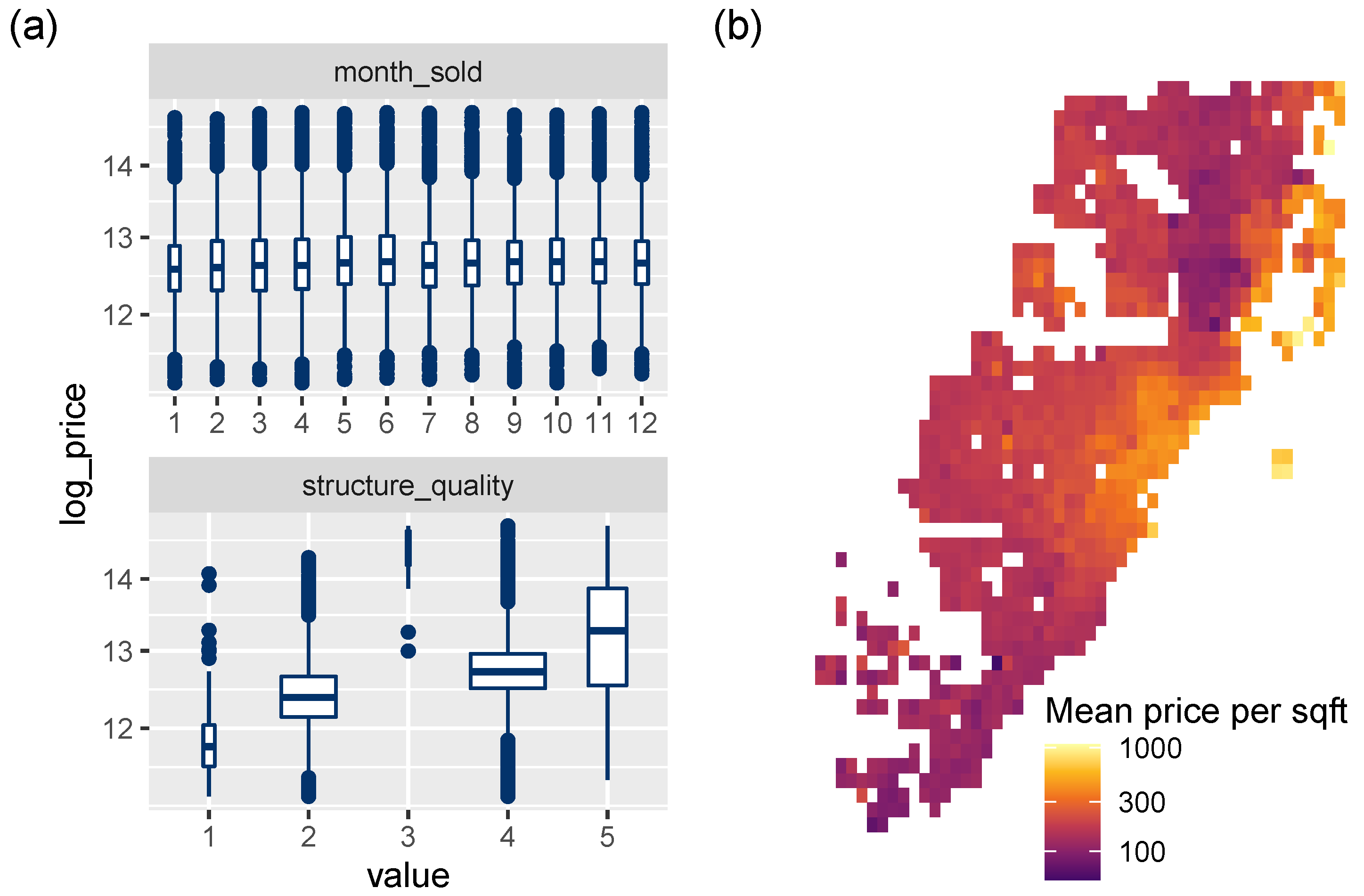
Figure 5.
(a) Association between discrete variables and the response log_price (boxplots). (b) Logarithmic heatmap of price per living area.

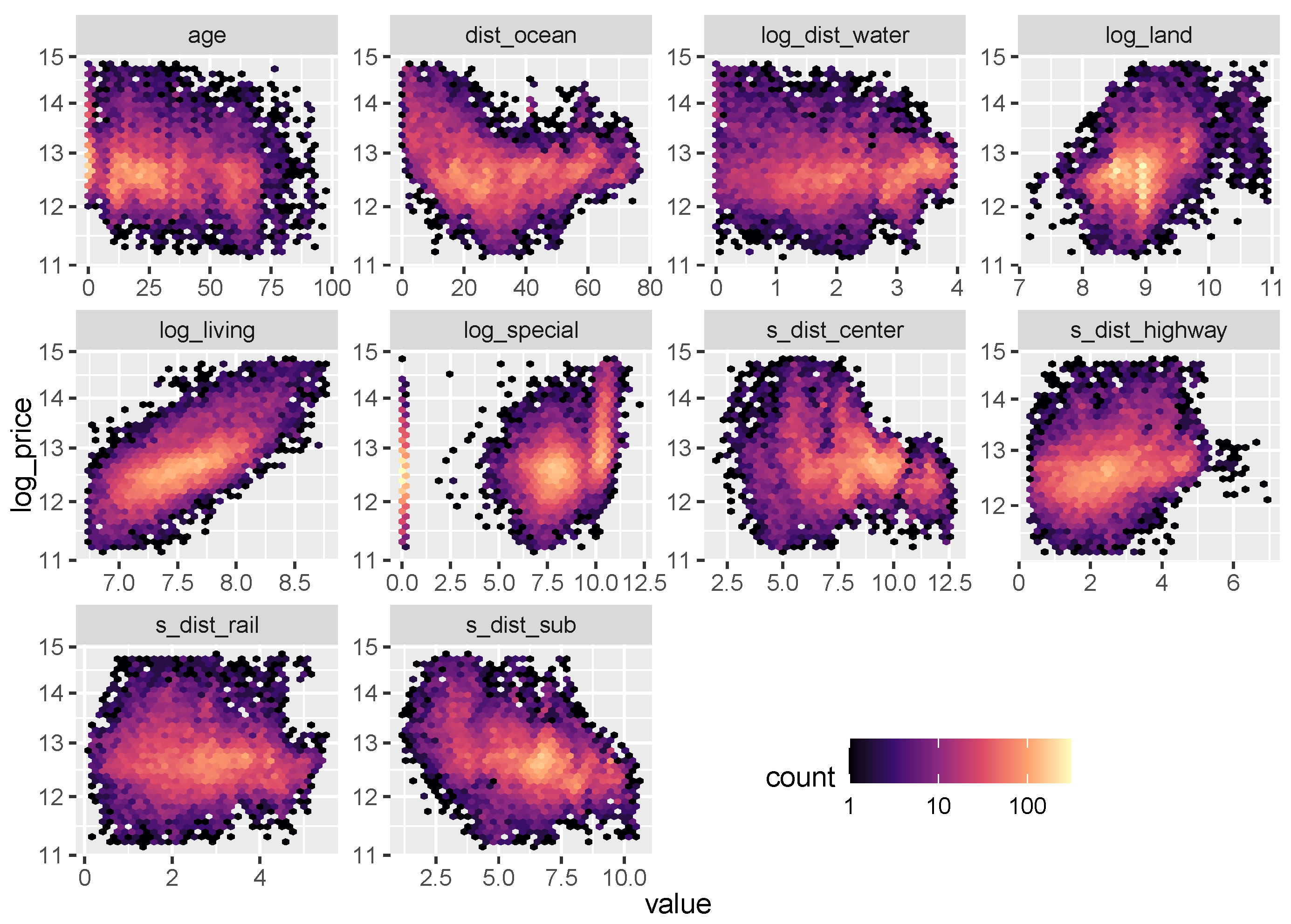
Figure 6.
Logarithmic heatmaps between the response log_price and the continuous variables (except latitude and longitude).
The set of locational variables corresponding to the feature vector is denoted by . Furthermore, observed values of any feature or feature vector are denoted by lowercase letters, such as or r.
3.2. Models
To illustrate the methods discussed in the previous sections, we consider six models:
- OLS: Linear regression benchmark with maximal interpretability.
- XGB (unconstrained): XGBoost benchmark for maximal performance.
- XGB STAR: XGBoost STAR model for high interpretability and performance.
- OLS with XGB loc: Linear model with location effects derived from XGB STAR.
- NN STAR: Deep neural STAR model.
- mboost STAR: mboost STAR model.
Details for each model are given below. Before fitting the models, the dataset was randomly split into 80% training and 20% test observations. The test dataset was used solely for evaluating the performance of the models, not for tuning them.
As a simple benchmark with maximal interpretability, we consider the OLS regression with time dummy effects g
fitted with R function lm(). This model does not use latitude/longitude, as there is no obvious way to represent them in this case.
To get a rough benchmark of the maximally achievable model performance, we consider the unconstrained XGBoost model, XGB (unconstrained), with learning rate 0.1. Its most relevant hyper-parameters (including tree depth, ridge and lasso regularization, and column and row subsampling) were tuned on the training data by a randomized search using five-fold cross-validation. A suitable number of trees (469) was chosen by early stopping on the cross-validation score. After tuning, the model was refitted on the full training data. The calculations were made with the R package xgboost (Chen et al. 2021) using squared error loss.
The next model considered (XGB STAR) is a STAR model fitted with XGBoost and interaction constraints to enforce time and building characteristic effects to be additive. Only the locational factors are allowed to interact with each other. The structured model equation follows the form of Equation (1):
In this way, the feature sets corresponding to the model components form a partition, which holds for all STAR models used in our case studies. Using the same learning rate and tuning strategy as the unconstrained XGBoost model, the cross-validated optimal number of trees (1583) was clearly higher to compensate for the additivity constraints.
From the XGB STAR model, we extracted the centered encoder using Algorithm 1. The values of this function represent the combined effect of all location variables, which we plugged as a derived feature into the OLS with XGB loc regression:
as outlined in Remark 4. This model can be viewed as a smoothed, linearized version of the XGB STAR model.
The remaining two models show alternative ways to fit a STAR model. Like the OLS with XGB loc model, they are constrained to have linear effects for the building characteristics. The first of these models is a neural network (NN STAR) with the equation
which is depicted in Figure 7. The architecture of the location sub-network (three hidden layers having 12-6-3 non-intercept nodes and hyperbolic tangent activations), the learning rate (0.003), and the number of epochs (105) were chosen by simple validation on the training data. As a loss function, the squared error was used. The model has 231 parameters, most of which are used to represent the location sub-network. Time is represented by an embedding layer. We used the R package keras (Allaire and Chollet 2021) to fit the model via TensorFlow. This model serves as alternative to XGB STAR, but is not expected to be as accurate for a sample of this size. Following the recommendation in LeCun et al. (2012), we scaled numeric input features to a common scale in order to improve the convergence properties.
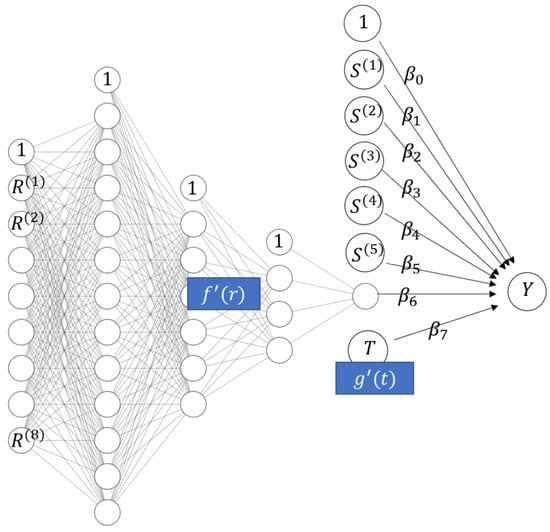
Figure 7.
Architecture of the neural network STAR model of Miami house prices.
Remark 6.
Neural networks are often biased in the sense that their average prediction on the training data is different from the corresponding average response; see Wüthrich (2020) for ways to address this. We skipped this calibration step for simplicity.
The last model considered (mboost STAR) is a model-based booster fitted with the R package mboost (Hothorn et al. 2021):
Per boosting round, the locational variables R are represented by a decision tree, while the other variables are fitted by linear functions via unpenalized least squares (time T is internally dummy encoded). The main tuning parameter, the number of boosting rounds, was chosen by five-fold cross-validation and amounted to 1022 rounds at a learning rate of 0.1. The tree depth was set to five in order to allow for a flexible representation of the location variables comparable to the XGBoost models.
3.3. Results
The models were evaluated on the 20% test data and interpreted using the flashlight package (Mayer 2021).
3.3.1. Performance
Model performance is measured by out-of-sample root mean square error and R-squared (Table 4). The constrained, highly structured XGBoost STAR model performs almost as well as the unconstrained, fully flexible XGBoost model, which is remarkable: By sacrificing only 0.2 percentage points of out-of-sample R-squared, we were able to create a transparent model (see figures below), avoiding the typical trade-off between performance and interpretability. The OLS with XGB loc model provides a model that is even simpler to interpret, here at the cost of one percentage point of R-squared. The other STAR models perform worse, but, as usual, such comparisons must be undertaken with care due to the different tuning techniques and different structures of the model components. Thus, we purposely do not show the p values for pairwise comparisons of performance.
Table 4.
RMSE and R-squared evaluated on the Miami hold-out dataset.
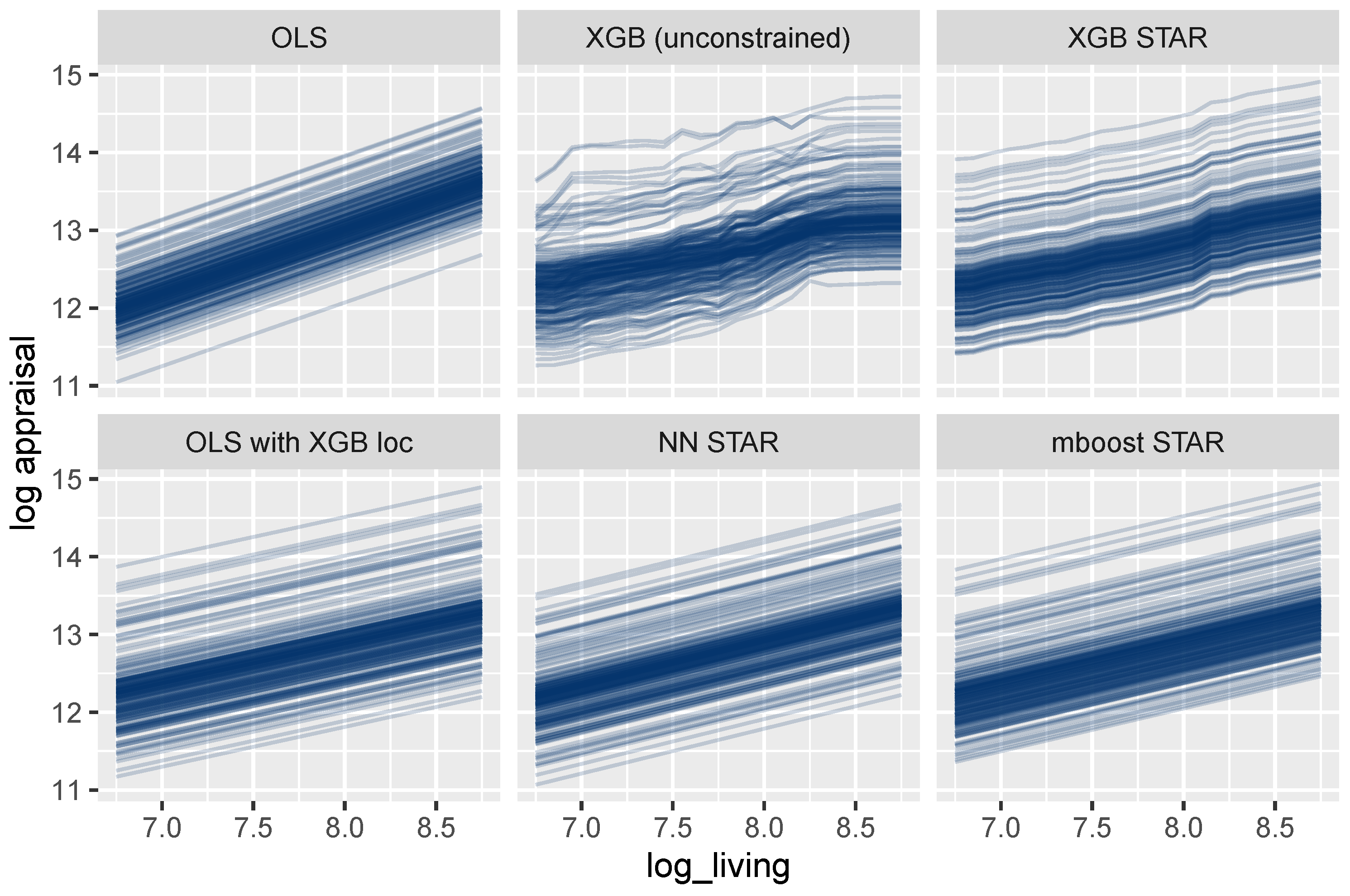
3.3.2. Effects of Single Variables
As outlined above, feature effects in general ML models can be described by ICE curves (Goldstein et al. 2015). Figure 8 shows such curves for the living area. One curve explains how the predicted logarithmic price of a selected house changes for different values of the living area, keeping all other feature values fixed. As expected, the curves are parallel for all models that are additive in the living area, which is the case for all models except the unconstrained XGBoost model. For these models, the effect of the living area can thus be described in a fully transparent way by studying a single ICE curve. The same holds for each other building characteristic and time.
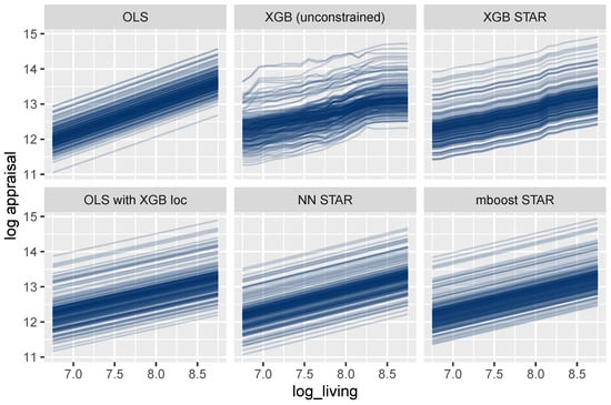
Figure 8.
ICE curves for log_living. All curves are parallel and simple to interpret, except for the unconstrained XGBoost model.
For the mboost model, the deep neural net, and the two linear regressions, the curves are linear, leading to maximum interpretability. In these cases, the effect of the living area could be described by a single number, namely, the slope of any ICE curve, which equals the corresponding model coefficient.
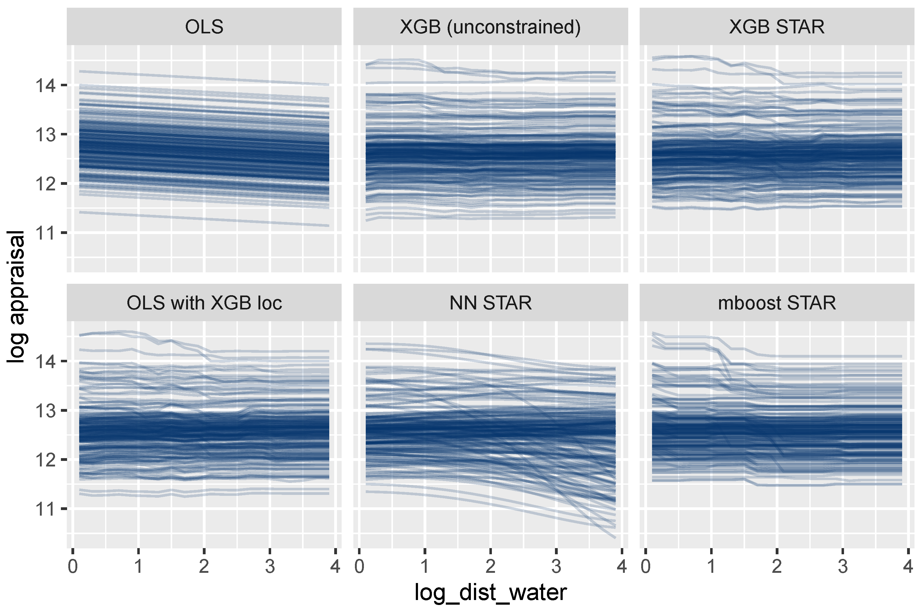
A completely different picture emerges for log_dist_water (Figure 9). The ICE curves of this location variable are parallel only for the oversimplified OLS model. The other models allow this feature to interact with other features, leading to non-parallel curves. Using the terminology discussed above, the feature set {log_dist_water} is not encodable for these models. Consequently, a single ICE curve or a PDP cannot provide a complete description of its modeled effects. We will, however, show that the combined effect of all location features can be described transparently by a single visualization.
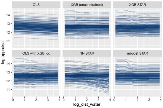
Figure 9.
ICE curves for the locational variable log_dist_water show non-additive effects, except for the OLS regression.
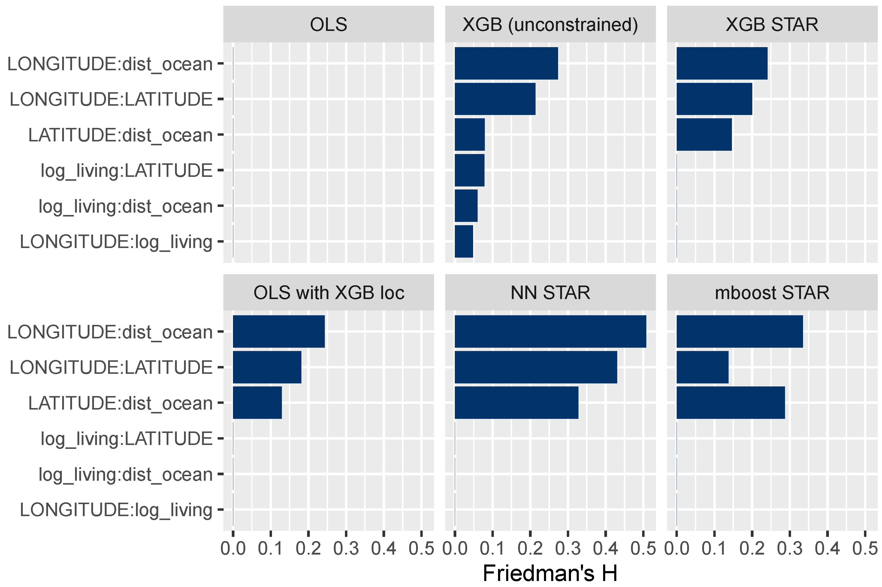
3.3.3. Interaction Effects
The field of explainable ML offers different ways to study interaction effects; for instance, multidimensional ICE curves or Friedman’s H measure of interaction strength (Friedman and Popescu 2008), which we consider here. Figure 10 shows H for selected variable pairs. A value of 0 means that there are no interactions, while higher values represent stronger interactions relative to the two corresponding main effects. The results in Figure 10 suggest that all STAR models have been correctly specified. For instance, the interaction strength between the living area and latitude is 0 for all models, except for the unconstrained XGBoost model.

Figure 10.
Friedman’s H measure of interaction strength for selected variable pairs. The STAR models appear to be correctly specified.
3.3.4. Supervised Dimension Reduction and Location Effects
As noted in the discussion of the methodology, STAR models can sometimes be used for supervised dimensionality reduction. For the STAR models in this case study, this is done by representing all location variables R with a single model component. Once fitted, the values of that component serve as a one-dimensional representation of the set of locational variables. We used Algorithm 1 to extract centered encoders of R from each of the three explicit STAR models. To illustrate the workflow of Remark 4, the encoder of XGBoost STAR was subsequently plugged as a derived feature into the simplified OLS with XGB loc model, with excellent results (see above).
Furthermore, since there is a trivial mapping from the two features of latitude and longitude to the encodable set of location features , we were able to use the projection trick described above to provide a fully transparent description of the combined location effects. To do so, we visualized as heatmaps the values of the centered encoders of the three STAR models (XGB STAR, NN STAR, and mboost STAR) over all latitude/longitude pairs appearing in the full dataset (Figure 11).
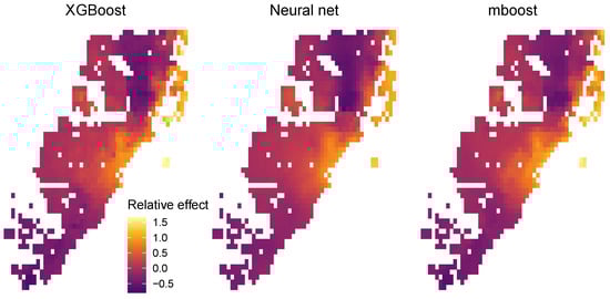
Figure 11.
Relative location effects extracted from the three STAR models: XGB STAR, NN STAR, and mboost STAR.
Since the model response is logarithmic, the values of the centered encoders can be interpreted as relative location effects. For example, a location with value 0.2 would be about 20% above the average price level of Miami. The results in Figure 11 look highly plausible. Due to its superior performance, the relative price map produced by the XGBoost STAR model shows slightly more pronounced effects, e.g., very high prices for the exclusive area Key Biscayne.
4. Case Study 2: Swiss Housing Data
4.1. Data
Our second case study uses a rich geocoded dataset covering over 67,000 houses sold at arm’s length between 2010 and 2021 in Switzerland. It was provided by the Informations- und Ausbildungszentrum für Immobilien AG (IAZI), a Swiss company specializing in property valuation. The median house has 5.5 rooms, 150 of living area, and a lot size of 576 , and was 34 years old at transaction time. For confidentiality reasons, the sales prices were multiplied by a fixed, unknown constant.
The aim of this second case study is to derive models for the median logarithmic sales price, conditional on the following 90 features:
- Twelve pre-transformed property characteristics (logarithmic living area, number of rooms, age, etc.) represented by the feature vector .
- Transaction time (year and quarter) T.
- A set of 25 untransformed locational variables mostly available at the municipal level, such as the average taxable income or the vacancy rate.
- Latitude and longitude.
- For 25 points of interest (POIs), such as schools, shops, or public transport, their individual counts within a 500 m buffer.
- The distance from the nearest POI of each type to the house (maximum 500 ).
The feature set containing time T and all 77 locational variables is denoted as and the corresponding feature vector as R. As usual, we denote observed values of features by lowercase letters.
4.2. Models
Our house price models have the structure
where the response Y equals the logarithmic sales price. More specifically, we consider these three models:
- LGB (unconstrained): LightGBM benchmark for maximum performance. Hyper-parameter tuning was done by stratified five-fold cross-validation, using a learning rate of 0.1 and systematically varying the number of leaves, row and column subsampling rates, and L1 and L2 penalization. As for the XGBoost models in the first case study, the number of trees (1918) was chosen by early stopping on the cross-validation score. The model was fitted with the R package lightgbm (Ke et al. 2021), using the absolute error loss in order to provide a model for the conditional median (Table 2).
- LGB STAR: LightGBM STAR model for high interpretability and performance. This is built similarly to the first model (with 2225 trees), but with additive effects for building variables enforced by interaction constraints. Locational variables and transaction time were allowed to interact with each other. This leads to a model of the form
- QR with LGB loc: Linear quantile regression (Koenker 2005) with time-dependent location effects derived from LGB STAR model, using Algorithm 1 to extract the centered encoder . The model equation is thusand can be viewed as a linearized LightGBM quantile regression model. The model was fitted with the R package quantreg (Koenker 2021).
For the sake of brevity, we do not consider deep learning and mboost in this case study. The models were tuned and trained on 80% of all observations and evaluated on the remaining 20%. The data split and the cross-validation folds (for tuning LightGBM) were created by stratification on ten quantile groups of the response variable to improve balance across subsamples.
4.3. Results
4.3.1. Performance
As in the first case study, the model performance is evaluated on the independent test dataset. In line with the aim of modeling a conditional median, the relevant performance measure will now be the mean absolute error (MAE), while the RMSE is added for information only. Table 5 shows that the constrained, highly interpretable LightGBM STAR model performs only slightly worse than the unconstrained model. The loss in performance of the linear quantile regression with the LightGBM encoder is larger, but still surprisingly small. It could be improved by adding non-linear terms. An MAE of 0.168 implies, thanks to the logarithmic response, that the average relative appraisal error of the LightGBM STAR model is about %.
Table 5.
MAE and RMSE evaluated on the Swiss hold-out dataset.
4.3.2. Effects of Additive and Non-Additive Features
Figure 12 shows ICE curves of the logarithmic surface area for a small random sample of properties. As expected, the unconstrained model shows non-parallel curves, and thus, its feature effects are difficult to interpret. In contrast to this behavior, the curves for the LightGBM STAR model are intrinsically parallel, leading to a fully transparent description of the effect. The corresponding effect in the linear quantile regression can be described by a single number, namely, the slope of the lines.
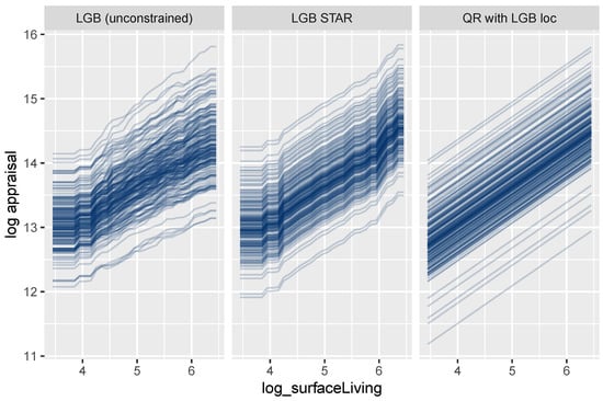
Figure 12.
ICE curves for logarithmic living area.
On the other hand, the effect of the transaction time T is non-additive for all three models due to interaction effects with location (Figure 13).
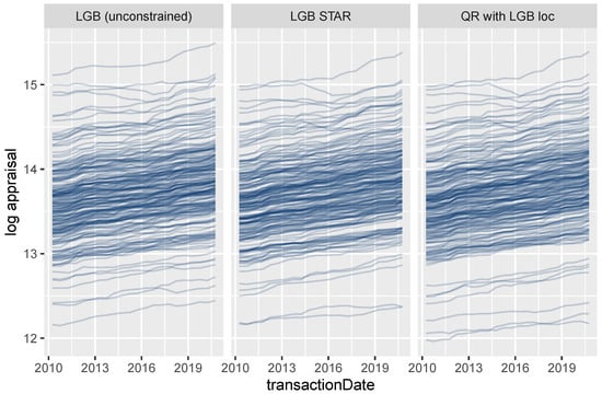
Figure 13.
ICE curves for the date of transaction.
4.3.3. Extracting Time-Dependent Location Effects
In this case study, the centered encoder serves as a one-dimensional representation of both time and locational effects. In the QR with LGB loc model, we followed the workflow of Remark 4 and plugged the encoder as a derived feature into a simple-to-interpret linear model while retaining complex time-varying locational effects.
Furthermore, since the large feature set , consisting of 77 locational features plus time T, has the natural low-dimensional representation (, Latitude, Longitude), we can use the projection trick discussed above to visualize the combined effect of R. To do so, we plot heatmaps of the centered encoder over all unique combinations of latitude and longitude and for different values of T. Figure 14 shows realistic relative price maps with the usual hotspots of Zurich, Geneva, and St. Moritz. An increasing price trend is clearly visible. Due to interaction effects between time and location, the time trend varies across locations.
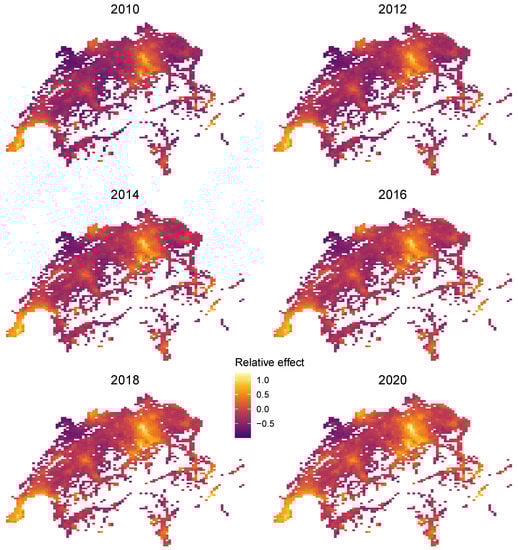
Figure 14.
Time-dependent relative location effects in Switzerland extracted from the LightGBM STAR model.
Remark 7 (Regional hedonic indices).
In Figure 14, we visualized regional effects for selected time points. Similarly, it would be straightforward to visualize time effects for selected addresses. In fact, each ICE curve in Figure 13 shows an address-specific time effect. Regional indices at some administrative unit (e.g., the canton) could be created by a STAR model using additive components for the object characteristics, one component for all regional effects, and one component for canton and time.
5. Discussion and Conclusions
We have shown that, thanks to interaction constraints, the two high-performance gradient boosting libraries XGBoost and LightGBM can be used to create highly intelligible and accurate GAM and STAR models. In contrast to traditional ways of fitting such models, tree-based additive components can use large groups of features. The combined effects of such groups can be extracted as derived one-dimensional features and used in subsequent analyses, such as in a simplified linear regression model.
This paper is the first to apply these techniques to house price valuation, where a large group of location features that contribute to land value can be represented with maximum flexibility while restricting the effects of each building characteristic to be additive for full transparency.
Our case studies illustrate the usefulness of these techniques, as well as their flexibility. In the Miami case study, we found that the XGBoost methods performed very well with respect to predictive accuracy, with a constrained model that allowed for some transparency performing nearly as well as an unconstrained model that was completely opaque. Moreover, an OLS model with a single location variable derived from the constrained XGBoost model also performed quite well. In the Swiss case study, the highly interpretable LightGBM STAR (constrained) model performed almost as well as the unconstrained LightGBM model. A linear regression model with a single location variable derived from the constrained model also performed well. In general, these approaches combine two desirable features: high predictive accuracy and interpretability for selected variables.
A further application in real estate modeling would be to add high-dimensional numeric information extracted from text and/or images—just like a group of locational features—to the model, without reducing the interpretability of the other covariates. The techniques are not only relevant in situations involving housing data. Consider, for example, automobile insurance pricing models, where one could represent driver characteristics in an additive and fully transparent way while letting characteristics of the car interact freely with each other. Finally, further research is needed to identify applications where structured deep learning would outperform gradient boosting with interaction constraints.
Author Contributions
Conceptualization, M.M., S.C.B., M.H. and D.S.; methodology, M.M., S.C.B. and M.H.; data curation, S.C.B. and D.S.; writing—original draft preparation, M.M., S.C.B. and M.H.; writing—review and editing, M.M., S.C.B. and M.H.; visualization, M.M. All authors have read and agreed to the published version of the manuscript.
Funding
This research received no external funding.
Data Availability Statement
The complete R code of the case study is available at https://github.com/mayer79/star_boosting (accessed on 26 September 2021). The dataset can be found at https://www.openml.org/d/43093 for research purposes (accessed on 24 September 2021).
Acknowledgments
We thank Nicola Stalder and his IAZI team for preparing the dataset for the Swiss case study. The authors are grateful to the referees, whose feedback and comments have improved the quality of the paper.
Conflicts of Interest
The authors declare no conflict of interest.
References
- Abadi, Martin, Paul Barham, Jianmin Chen, Zhifeng Chen, Andy Davis, Jeffrey Dean, Matthieu Devin, Sanjay Ghemawat, Geoffrey Irving, Michael Isard, and et al. 2016. Tensorflow: A system for large-scale machine learning. Paper presented at 12th USENIX Symposium on Operating Systems Design and Implementation (OSDI 16), Savannah, GA, USA, November 2–4; pp. 265–83. [Google Scholar] [CrossRef]
- Agarwal, Rishabh, Levi Melnick, Nicholas Frosst, Xuezhou Zhang, Ben Lengerich, Rich Caruana, and Geoffrey E. Hinton. 2021. Neural additive models: Interpretable machine learning with neural nets. Advances in Neural Information Processing Systems 34. [Google Scholar]
- Allaire, Joseph J., and François Chollet. 2021. Keras: R Interface to ’Keras’, R Package Version 2.4.0; Available online: https://CRAN.R-project.org/package=keras (accessed on 1 June 2021).
- Arik, Sercan Ömer, and Tomas Pfister. 2019. Tabnet: Attentive interpretable tabular learning. arXiv arXiv:2004.13912. [Google Scholar]
- Bühlmann, Peter, and Torsten Hothorn. 2007. Boosting Algorithms: Regularization, Prediction and Model Fitting. Statistical Science 22: 477–505. [Google Scholar] [CrossRef]
- Biecek, Przemyslaw, and Tomasz Burzykowski. 2021. Explanatory Model Analysis. New York: Chapman and Hall/CRC. [Google Scholar] [CrossRef]
- Chen, Tianqi, and Carlos Guestrin. 2016. Xgboost: A scalable tree boosting system. Paper presented at 22nd ACM SIGKDD International Conference on Knowledge Discovery and Data Mining,KDD ’16, San Francisco, CA, USA, August 13–17; New York: Association for Computing Machinery, pp. 785–94. [Google Scholar] [CrossRef] [Green Version]
- Chen, Tianqi, Tong He, Michael Benesty, Vadim Khotilovich, Yuan Tang, Hyunsu Cho, Kailong Chen, Rory Mitchell, Ignacio Cano, Tianyi Zhou, and et al. 2021. Xgboost: Extreme Gradient Boosting, R Package Version 1.4.1.1; Available online: https://CRAN.R-project.org/package=xgboost (accessed on 1 June 2021).
- Din, Allan, Martin Hoesli, and André Bender. 2001. Environmental variables and real estate prices. Urban Studies 38: 1989–2000. [Google Scholar] [CrossRef]
- Fahrmeir, Ludwig, Thomas Kneib, Stefan Lang, and Brian Marx. 2013. Regression: Models, Methods and Applications. Berlin: Springer. [Google Scholar] [CrossRef]
- Friedman, Jerome H. 2001. Greedy function approximation: A gradient boosting machine. The Annals of Statistics 29: 1189–232. [Google Scholar] [CrossRef]
- Friedman, Jerome H., and Bogdan E. Popescu. 2008. Predictive learning via rule ensembles. The Annals of Applied Statistics 2: 916–54. [Google Scholar] [CrossRef]
- Goldstein, Alex, Adam Kapelner, Justin Bleich, and Emil Pitkin. 2015. Peeking inside the black box: Visualizing statistical learning with plots of individual conditional expectation. Journal of Computational and Graphical Statistics 24: 44–65. [Google Scholar] [CrossRef]
- Hastie, Trevor, and Robert Tibshirani. 1986. Generalized Additive Models. Statistical Science 1: 297–310. [Google Scholar] [CrossRef]
- Hastie, Trevor, and Robert Tibshirani. 1990. Generalized Additive Models. Hoboken: Wiley Online Library. [Google Scholar]
- Hothorn, Torsten, Peter Bühlmann, Thomas Kneib, Matthias Schmid, and Benjamin Hofner. 2021. Mboost: Model-Based Boosting, R Package Version 2.9-5; Available online: https://CRAN.R-project.org/package=mboost (accessed on 5 July 2021).
- Hothorn, Torsten, Peter Bühlmann, Thomas Kneib, Matthias Schmid, and Benjamin Hofner. 2010. Model-based boosting 2.0. The Journal of Machine Learning Research 11: 2109–13. [Google Scholar]
- Kagie, Martijn, and Michiel Van Wezel. 2007. Hedonic price models and indices based on boosting applied to the dutch housing market. Intelligent Systems in Accounting, Finance & Management: International Journal 15: 85–106. [Google Scholar] [CrossRef]
- Ke, Guolin, Damien Soukhavong, James Lamb, Qi Meng, Thomas Finley, Taifeng Wang, Wei Chen, Weidong Ma, Qiwei Ye, Tie-Yan Liu, and et al. 2021. Lightgbm: Light Gradient Boosting Machine, R Package Version 3.2.1.99; Available online: https://github.com/microsoft/LightGBM (accessed on 13 August 2021).
- Ke, Guolin, Qi Meng, Thomas Finley, Taifeng Wang, Wei Chen, Weidong Ma, Qiwei Ye, and Tie-Yan Liu. 2017. Lightgbm: A highly efficient gradient boosting decision tree. In Advances in Neural Information Processing Systems. New York: Curran Associates, Inc., Volume 30, pp. 3149–57. [Google Scholar]
- Koenker, Roger. 2005. Quantile Regression. Econometric Society Monographs. Cambridge: Cambridge University Press. [Google Scholar] [CrossRef]
- Koenker, Roger. 2021. Quantreg: Quantile Regression, R Package Version 5.86; Available online: https://CRAN.R-project.org/package=quantreg (accessed on 13 August 2021).
- LeCun, Yann, Léon Bottou, Genevieve B. Orr, and Klaus-Robert Müller. 2012. Efficient backprop. In Neural Networks: Tricks of the Trade, 2nd ed. Edited by G. Montavon, G. B. Orr and K.-R. Müller. Volume 7700 of Lecture Notes in Computer Science. New York: Springer, pp. 9–48. [Google Scholar] [CrossRef]
- Lee, Simon C. K., Sheldon Lin, and Katrien Antonio. 2015. Delta Boosting Machine and Its Application in Actuarial Modeling. Sydney: Institute of Actuaries of Australia. [Google Scholar]
- Lou, Yin, Rich Caruana, and Johannes Gehrke. 2012. Intelligible models for classification and regression. Paper presented at 18th ACM SIGKDD International Conference on Knowledge Discovery and Data Mining, KDD ’12, Beijing, China, August 12–16; New York: Association for Computing Machinery, pp. 150–58. [Google Scholar] [CrossRef] [Green Version]
- Malpezzi, Stephen. 2003. Hedonic Pricing Models: A Selective and Applied Review. Hoboken: John Wiley & Sons, Ltd., Chapter 5. pp. 67–89. [Google Scholar] [CrossRef]
- Mayer, Michael. 2020. Github Issue. Available online: https://github.com/microsoft/LightGBM/issues/2884 (accessed on 6 March 2009).
- Mayer, Michael. 2021. Flashlight: Shed Light on Black Box Machine Learning Models, R Package Version 0.8.0; Available online: https://CRAN.R-project.org/package=flashlight (accessed on 1 June 2021).
- Mayer, Michael, Steven C. Bourassa, Martin Hoesli, and Donato Scognamiglio. 2019. Estimation and updating methods for hedonic valuation. Journal of European Real Estate Research 12: 134–50. [Google Scholar] [CrossRef] [Green Version]
- Molnar, Christoph. 2019. Interpretable Machine Learning. Available online: https://christophm.github.io/interpretable-ml-book (accessed on 1 July 2021).
- Nelder, John Ashworth, and Robert W. M. Wedderburn. 1972. Generalized linear models. Journal of the Royal Statistical Society: Series A (General) 135: 370–84. [Google Scholar] [CrossRef]
- Nori, Harsha, Samuel Jenkins, Paul Koch, and Rich Caruana. 2019. Interpretml: A unified framework for machine learning interpretability. arXiv arXiv:1909.00922. [Google Scholar]
- Prokhorenkova, Liudmila, Gleb Gusev, Aleksandr Vorobev, Anna Veronika Dorogush, and Andrey Gulin. 2018. Catboost: Unbiased boosting with categorical features. Paper presented at the 32nd International Conference on Neural Information Processing Systems, NIPS’18, Montréal, QC, Canada, December 3–8; New York: Curran Associates Inc., pp. 6639–49. [Google Scholar]
- Rügamer, David, Chris Kolb, and Nadja Klein. 2021. Semi-structured deep distributional regression: Combining structured additive models and deep learning. arXiv arXiv:2002.05777. [Google Scholar]
- Sangani, Darshan, Kelby Erickson, and Mohammad al Hasan. 2017. Predicting zillow estimation error using linear regression and gradient boosting. Paper presented at the 2017 IEEE 14th International Conference on Mobile Ad Hoc and Sensor Systems (MASS), Orlando, FL, USA, October 22–25; pp. 530–34. [Google Scholar] [CrossRef]
- Umlauf, Nikolaus, Daniel Adler, Thomas Kneib, Stefan Lang, and Achim Zeileis. 2012. Structured Additive Regression Models: An R Interface to BayesX. Working Papers 2012–10. Innsbruck: Faculty of Economics and Statistics, University of Innsbruck. [Google Scholar]
- Wei, Cankun, Meichen Fu, Li Wang, Hanbing Yang, Feng Tang, and Yuqing Xiong. 2022. The research development of hedonic price model-based real estate appraisal in the era of big data. Land 11: 334. [Google Scholar] [CrossRef]
- Wood, Simon N. 2017. Generalized Additive Models: An Introduction with R, 2nd ed. Boca Raton: CRC Press. [Google Scholar] [CrossRef]
- Worzala, Elaine, Margarita Lenk, and Ana Silva. 1995. An exploration of neural networks and its application to real estate valuation. Journal of Real Estate Research 10: 185–201. [Google Scholar] [CrossRef]
- Wüthrich, Mario V. 2020. Bias regularization in neural network models for general insurance pricing. European Actuarial Journal 10: 179–202. [Google Scholar] [CrossRef]
- Yoo, Sanglim, Jungho Im, and John E. Wagner. 2012. Variable selection for hedonic model using machine learning approaches: A case study in Onondaga County, NY. Landscape and Urban Planning 107: 293–306. [Google Scholar] [CrossRef]
- Zurada, Jozef, Alan S. Levitan, and Jian Guan. 2011. A comparison of regression and artificial intelligence methods in a mass appraisal context. Journal of Real Estate Research 33: 349–88. [Google Scholar] [CrossRef]


Publisher’s Note: MDPI stays neutral with regard to jurisdictional claims in published maps and institutional affiliations. |
© 2022 by the authors. Licensee MDPI, Basel, Switzerland. This article is an open access article distributed under the terms and conditions of the Creative Commons Attribution (CC BY) license (https://creativecommons.org/licenses/by/4.0/).