Abstract
It is an open secret that most investment funds actually underperform the market. Yet, millions of individual investors fare even worse, barely treading water. Algorithmic trading is now so common, it accounts for over 80% of all trades and is the domain of professionals. Can it also help the small investor? Individual investors are advised to buy-and-hold an index fund or a balanced portfolio including stocks, bonds, and cash equivalents. That would ensure market performance. However, market indices also occasionally have deep drawdowns (such as the devastating market crash of 1929 and other so-called Black Swan events). In contrast to received wisdom, we argue with evidence from backtesting on major U.S. market indices, as well as some select stocks that simple ideas in rule-based market timing can in fact be useful. One can not only obtain good results, but outperform market indices, while, at the same time, reducing deep drawdowns, surviving Black Swan events.
1. Introduction
The financial market can be at once enchanting and dangerous. It is inhabited by two types of investors: professional institutional investors and traders, plus professional investment advisors, whose time frames are typically short (e.g., a year or less), and average small investors, whose time frames are (or ought to be) long, stretching to decades. The professional traders understand market volatility and generally use algorithmic trading to deal with it. That subject has a long and rich history and encompasses a wide array of automated trading practices and purposes, including sophisticated high-frequency trading (HFT) (performed in microseconds), market making, arbitrage, trend-following, and mean-reversion approaches. For the money management side, they have both managed accounts as well as machine-driven trading. By contrast, the small investor has limited knowledge of the market, finds volatility frightening, and has few tools at her/his disposal to make investment decisions. As of 2022, institutional investors make over 90% of stock trades today (Pan 2022). Algorithmic trading itself now accounts for an estimated 80% of all stock trades and 92% of foreign exchange (Forex) trades (Shadmehry 2021), and no doubt rising. In large, algorithmic trading is also controversial, in that if too much of the volume of trading becomes algorithmic and a market event occurs that triggers many sell signals simultaneously, it can rapidly tank the entire market before any human can intervene. Therefore, algorithmic trading has been blamed in part for the famous market crash of 19 October 1987, as well as partly for the Financial Crisis of 2008. Yet, it is all the rage among professionals. However, can it help the small investor? In the business of making money, this question seems infrequently asked.
A quick overview of algorithmic trading is given in (Seth 2022), while the books (Chen 2009; Halls-Moore 2010) give more background and programming tools. HFT and other algo trading is the domain of professional investment houses, dealing in stochastic calculus models or deep learning, and where split-second timing is money. In contrast, simple rule-based market timing, generating just a few trade signals a year to buy or sell, is our main interest, as it may apply to the small investor. Note that while sophisticated trading strategies generally involve learning parameters in a model (or even a full neural network) and require a learning phase before a live testing phase, simpler rule-based models require no training. Certainly, if buy or sell decisions can be systematized, it can take away any human (read emotional) input and turn it into computer code. Moreover, the execution of those trading decisions can itself be automated using computers. Detailed research by the Investment Company Institute (Investment Company Institute 2021) shows that, for individual investors, planning for retirement was cited by 95% of those surveyed, and 72% cited it as the primary goal. The next-highest cited primary goal (saving for emergencies) was only 6%. Thus, investors do mainly invest for the long-term. However, it seems that their investment habits may not reflect that and tend to be influenced by emotions, especially fear and greed (so much so that these have turned into indicators for pros). To help them, we focus here on the automation of trading decisions, rather than the execution. In the realm of algorithmic trading approaches fit for individuals, those related to market timing are among the most controversial, or even downright derided as a fool’s errand. “Forget Market Timing and Stick to a Balanced Fund”, proclaimed a NY Times article in 2014 (Richards 2014). “The stock market is a device for transferring money from the impatient to the patient.”—Warren Buffett. When the small investor does try to time the market, it may be based on emotion rather than any tested method, with disappointing results.
Rule 1: Buy low and sell high. This is really the only rule of investing. If only it were easy to do. That formula is of course the basis of a method called value investing, a well-known and successful investment practice wherein a detailed study of specific stocks and their expected future cash flows can be used to suggest a current price target, based on the present value of future returns; if that price target is in fact higher than the actual price, the stock is deemed a “value stock”; it then becomes of interest and is potentially worthy of buying. Later, if it gains some momentum (over time, perhaps years) and its price rises above a computed price target at that time, it may be time to sell it. While some of the most successful investors such as Warren Buffet indeed use this method (with impressive results), which can arguably provide the very best returns long-term, the typical investor has neither the time, skill set, nor patience to apply it. Such investors are rather more likely to follow a herd instinct, piling into stocks based on overheard tips or seeing stock prices rise. “Tesla is soaring… time to get some.” In fact, evidence clearly shows that typical investors tend to buy as the price is going up and sell as its going down, the reverse of value investors. This explains the poor performance results experienced by typical investors. They try to time the market, but get it wrong. Indeed, market timing is hard. Moreover, highbrow research purports to claim that, in fact, market timing is not only badly practiced, but effectively cannot be done.
Individual investors are thus widely advised—by financial advisory houses—to get a financial advisor (!), who may even suggest they can offer an annual 3% value-add to their returns (Vanguard Research 2019). Failing that, they would suggest using the simplest proven strategy: buy-and-hold, and to do so using a balanced portfolio including stocks, bonds, and cash equivalents such as money market funds. The most well-known example is the 60–40 rule, which suggests holding 60% of available funds in stocks and 40% in bonds. However, even then, precisely which stocks, bonds, etc., to buy and when to buy or sell are open and overwhelming questions for the typical investor, who indeed obtains unimpressive results—thus, again, investment is best left to the professionals. Against this background, is there any hope for the do-it-yourself small investor? Can market timing be at all a part of a DIY approach? First, since even professional investors generally underperform market indices, the first advice is to just invest in market indices! That will at least ensure one obtains market performance, which is already better than not only most small investors, but most professional ones. This advice is not new, but given the actual poor returns of typical investors, it bears repeating, and top investors such as Warren Buffett do suggest it. However, this approach cannot obtain better-than-market returns, which investors like Buffett aim to get. In fact, by investing in an index fund, one effectively buys bits of every stock in the index, both the strong and weak performers. To do better than the index, one must find a way to identify the likely strong performers from the weak ones—what Buffett and others practice through their value analysis. From Buffett’s point of view, diversifying for its own sake would only dilute the returns, and he has railed against it. In this sense, diversify only to cover ignorance. Unfortunately, ignorance of the market is rampant among average investors.
Even so, index fund returns are good returns, and would serve the typical investor well if held long-term. Yet, there is one other problem with index buy-and-hold investing. As is well known, market indices occasionally have very deep drawdowns (such as the devastating market crash of 1929, which took decades to recover from), for which the typical small investor has little protection, either emotionally or financially. If one must withdraw invested funds while the market is down, one can suffer massive losses, which can be crippling. If one pursues index investing, then buy-and-hold cannot be a workable strategy during all market conditions. The fact is no one knows when major downturns may happen, only that they will. However, one needs a way to get out before things get bad. Can there be a middle ground way that does that? The consensus seems to be no. However, in contrast to the received wisdom, we argue, with evidence by backtesting on major U.S. market indices, that simple ideas in market timing can, in fact, be useful. One can not only obtain good results, but even outperform market indices, while at the same time reducing the deep drawdowns. How is this possible, when so much expert advice is contrary to this? One may need to revisit who benefits from that advice.
The rest of this paper is organized as follows. Section 2 reviews the disadvantages for the average investor in terms of what to buy and sell, and when. Section 3 reviews the limitation of actively managed funds as well. This review of investor and managed fund performance mainly serves to highlight a persistent, yet under-served problem and a gap in the research: how to help the small investor obtain better results. These investors try to time the market, but do it badly. Section 4 discusses academic research suggesting that market timing is effectively impossible. The vast literature of algorithmic trading geared almost exclusively toward short-term trading by investment houses is of little use to them. With this negative background, Section 5 presents our study of one form of algorithmic trading: market timing, with the explicit aim of helping the small investor. We introduce what market timing is, review how to measure the performance of such a trading system, cover a little history of major U.S. market indices, and delve into specific classes of market timing systems, focusing on those based on moving average analysis. Our main thesis is that an elementary form of market timing can be quite effective for long-term investing. In Section 5, Section 6, Section 7 and Section 8, we present a variety of new results, allowing for higher interest rates, covering timescales in decades, up to 93 years, showing the strong performance of our market timing system on SPX and IXIC indices, as well as some common U.S. stocks. Section 8 and Section 9 present a summary of the results and the conclusions. Some natural directions for extensions and further research are presented.
Our contributions are as follows. Unlike most of the algorithmic trading literature, we specifically address the needs of individual investors aiming for long-term investing. The most studied timing systems using moving averages generally use two time periods. We develop new, slightly more sophisticated rule-based methods based on up to four moving averages, which are more sensitive, yet consistent. Yet, by making only a few trading decisions a year on average, our system can be easily followed by individuals (upon advice), which moreover provides both strong returns and reduced drawdowns over decades. While many papers claim gains over the market using algorithmic trading, our method stands out as one a small investor can use at home.
2. Disadvantages for the Individual Investor
The rich get richer and the poor get poorer and, in the meantime, in between time, ain’t we got fun, is a famous verse from the 1920 song Ain’t We Got Fun, featured in the 1974 film The Great Gatsby. In simple terms, it suggests the economic ladder is tricky to climb, and slippery on the lower rungs. While we are not pursuing social commentary, in terms of investing, it is now well documented that small investors do poorly. We know why. First, just the size of the market alone is confounding. There are some 4K stocks, over 7K mutual funds, and roughly 3K exchange traded funds (ETFs), just in the U.S. To the typical investor, what to buy can be decided on hearsay. That is where value analysis, used by professionals, but unfamiliar to the typical investor, is key. Second, and crucially, when to buy, and sell, is a total mystery to the typical investor. They have heard of our Rule 1, but do not know how to execute it. Therefore, they tend to follow the herd. When prices rise, they buy; when they fall, they sell. This behavior is known as return-chasing and, according to an economic blog by the St. Louis Fed (Chien 2014), is a significant cause of the underperformance by the average investor since fund performance often reverts to the mean. According to senior economist Chien, net flows into funds in any given quarter (1992–2011) positively correlated with the performance of funds the previous quarter, with a correlation coefficient of 0.49. In short: (1) they tend to get in and out at the wrong time (Figure 1); (2) they tend to chase good past returns, which, due to frequent reversion to the mean, works against them (Figure 1 and Figure 2); (c) indeed, they obtain poor to very poor investment results. For many reasons, it would be beneficial to have tools to help boost their investment performance. That is especially true in timing the market.
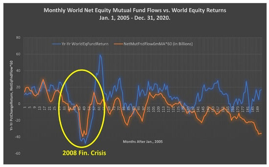
Figure 1.
Net money flows into/out of world equity mutual funds are seen to be the reverse of what value investing would suggest, with flows well correlated with performance. Based on data from the Investment Company Institute (Investment Company Institute n.d.).

Figure 2.
The 20-year performance of various investments (1992–2011) and the poor returns of the average investor. Sources: BlackRock, Bloomberg, Informa Investment Solutions, Dalbar (Ro 2013).
Small individual investors are prone to emotional trading, which, in financially stressful times, can drive them to the most ill-advised market actions (the pros would say, “because they were unadvised”). The occasional occurrence of major market downturns, familiar to the professionals, but frightening to the average investor, can spell investment doom. “Psychological factors such as fear often translate to poor timing of buys and sells.”—BlackRock.
In another study by the Boston-based research company Dalbar, Inc., covering the 20-year period ending 31 December 2019, the S & P500 returned 6.06% annually, while the individual investor earned just 4.25% (Anspatch 2021; Fidelity 2021). In yet another study by using results from the Investment Company Institute (Investment Company Institute 2021), for the 30-year period ending 31 December 2016, the average equity investor gained 3.98%, while the SPX gained 10.16% per yr. (Roberts 2017); see Figure 5. For fixed-income investors, the figure was a downright dismal, 0.57%, while inflation for those 30 years was 2.65%, and a Bloomberg-Barclays bond index was up 6.34%.
This massive under performance by millions of ordinary investors of modest means, for a 30-year period, is an unregulated national loss, and a call to action.
Similarly, Figure 3 is a chart based on a Dalbar, Inc. study, as reported in a marketing blog by Fidelity (2021). While the performance of the average investor is indeed dismal, note that even for the benchmark index, the S&P500, the results are rather lackluster (and less than its performance over longer periods). The reason is that this particular period included two major market events—called Black Swan events—the 2000 Dotcom Crash and the 2008 Financial Crisis. Note that among major Black Swan events, the sudden market crash of Monday, 19 October 1987, was especially noteworthy. In one day, the Dow fell nearly 22%. Entire fortunes were wiped out, with no warning. These Black Swan events will feature in our graphs later. As it happens, this particular event did not persist, nor cause a recession, and the stock market recovered in an orderly manner. However, such events can wreak havoc for investors, especially if they are emotional in their decisions. In Figure 3, we see that average investors did worse than benchmark indices, though note that, for this period, even the indices had muted performance numbers. In any case, the unadjusted return of the S&P500 index over longer periods (e.g., last 50 years) is about 10%, useful for the rare patient investor. However, the typical, impatient individual investor is saddled with under-performance, often below inflation rates. In effect, they run out to buy goods when they are expensive, only to return them (at lower prices) when they go on sale. Against this trap, the massive financial services industry is only too glad to lend a hand, for a fee. After all, the serious business of investing should be left to the professionals, who, by dint of deep research and well-rounded experience, know what to buy, sell, and when.

Figure 3.
Twenty-year return for the average investor in various investment types, against stock/bond benchmarks, based on research by Dalbar, Inc., as reported in (Fidelity 2021). Note that even the performance of the benchmark S&P500 index was muted in this period, as it contained both the 2000 Dotcom crash and the 2008 financial crisis events.
3. Active Funds Are No Panacea Either
However, it turns out, that this is not true either. While funds do outperform individual investors, they typically also underperform against the benchmarks that they work against. This odd fact is also widely known in professional circles (but never mentioned in marketing materials). There are many sources for this information, but we will turn to a definitive study, the SPIVA: 2021 Full-Year Active vs. Passive Scorecard (Coleman 2022). For the 20-year period ending 31 December 2021, fully 95% of all actively managed U.S. equity funds underperformed their benchmarks on a risk-adjusted basis (and 90% even without risk adjustment). If one looks at large-cap funds, the performance of active funds is even worse. Sadly, paying a professional does not seem to pay. Therefore, what is an individual to do? Easy—just obtain index funds and hold them! However, the typical investor seems short on patience (see Figure 4).
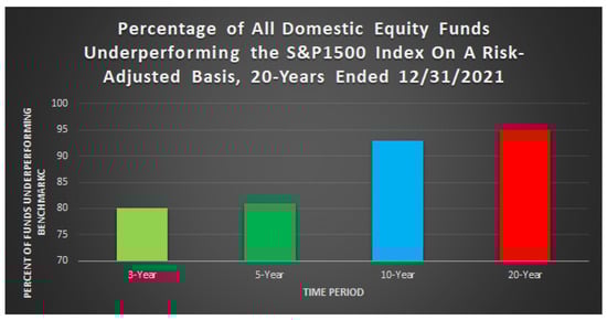
Figure 4.
SPIVA research results on active funds vs. index benchmarks over the 20-year period ending 31 December 2021. Measured on a risk-adjusted return basis, a staggering 95% of all domestic equity funds underperformed a key benchmark (S&P 1500) over the 20-year period. Even when measured in absolute terms, that figure is still 90%. Finally, similar results hold in all categories of managed funds underperforming their respective benchmarks (Coleman 2022).
4. Why Market Timing Is Bad
We know that the individual investor is bad at market timing, but so are many professionals. Is market timing inherently bad or ineffective? An online blog (Roberts 2017) documents that individuals in fact deeply underperform benchmarks such as the S&P500 index. This is believed to be due to investors getting spooked by downturns and selling. As Finance professor Estrada (Estrada 2008) explains, Black Swan events are a key killer of market timing approaches, which often spook both average investors and savvy professionals (e.g., hedge funds) alike. Moreover, such events occur much more often than standard Gaussian models would suggest, making market timing treacherous. He states simply, “black swans render market timing a goose chase.” This poses a fundamental challenge for us: Can we find a way in market timing strategies to negotiate through Black Swans successfully? That would be a game changer. If we can negotiate them, then that implies that these events arrive after subtle hints that we must find a way to pick up on.
However, the mantra of market timing is easy to state: be in the market when it starts going up and be out as it starts to go down. Put this way, it is just a restatement of Rule 1. Investors try this, but act too late! However, is market timing impossible, or inherently ineffective? In a series of two important papers in 1981, Nobel Prize-winning economist Robert Merton (MIT) made that case, by building a mathematical theory using stochastic calculus to study the performance of market timing (Henriksson et al. 1981; Merton 1981). First, for market timing to be successful, it is the same as being able to forecast future market movements better than by chance alone. In his theory, the investment returns of even a perfect market timer are shown to be equivalent to those of certain options that are “undervalued”, that is, below the fair value that would be given, for example, by Black–Scholes analysis. The implication seems to be that it is unlikely to find such a perfect market timer, whose short-lived opportunities would disappear as soon as markets returned to efficiency. Moreover, such a market timer would charge a management fee, which he/she then estimates, which would in effect kill any chance for an investor subscriber to such a market timing service to realize any value. (Prof. Merton makes no mention of an unskilled individual investor as a possible market timer, only as an investor.) Thus, his propositions often end like the one below (Figure 5):
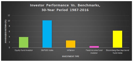
Figure 5.
Individual investors consistently and deeply underperform buy-and-hold in index funds, for (a) stocks and (b) bonds, as reported in (Roberts 2017). Notice that this period included most of the big Black Swan events, which often send individual investors selling at just the wrong time. Fixed-income investors did not even tread water vs. inflation.
Proposition III.6 (Merton): If a market timer’s forecasts are based solely on public information, then the value of the forecast is zero (Merton 1981).
Merton, in effect, put the nail in the coffin of successful market timing. If it is at all possible, it is equivalent to utilizing rare, undervalued options. If the timing forecasts are based only on public, e.g., not insider, information, they can be of zero value to investors. In short, it is useless. There is no end to the derision that the field attracts.
“The only value of stock forecasters is to make fortunetellers look good.”—Warren Buffett. “A decade of results throws cold water on the notion that strategists have any special ability to time the markets.”—Wall Street Journal. “Far more money has been lost by investors preparing for corrections, or in trying to anticipate corrections, than in corrections themselves.”—Peter Lynch. “Let’s say it clearly: no one knows where the market is going—experts or novices, soothsayers or astrologers. That’s the simple truth.”—Fortune. “Don’t get me wrong, it’s only human to find the promise of market timing so appealing. It seems so obvious in hindsight. When we look back, we can see clearly that we all should have been selling stocks in 2007, and buying them again in 2009. However, if you go back to that time period, the facts show that most of us weren’t, because we didn’t know at the time that we’d reached the peak or the bottom. That’s the reality.”—NYTimes. All quotes are from (Richards 2014).
However, could we have known, at least in some limited way? Note first that market timing is not predicting the market direction going forward, only developing probabilistic models of whether to be in or out of the market just on a given day.
5. Why Market Timing May Be Good
“Few investment strategies have a worse reputation than market timing.”—P. Shen, economist, Federal Reserve Bank of Kansas City, 2002.
The difference is that, this time, it is the opening line of a paper entitled, “Market Timing Strategies That Worked”, by economist P. Shen (2002). It goes on to develop market timing strategies that would have beaten market indices, for real data for the 30-year period 1970–2000. “The simplicity and effectiveness of these strategies challenge the notion that market timing is inherently difficult.” (Shen 2002). His methods are based on examining the spreads between the E/P ratio (the inverse of the more common P/E or price/earnings ratio) and interest rates and their predictive capabilities for future price movements. In particular, he uses spreads based on the difference between S&P E/P ratios and interest rate surrogates over two time frames: yields on 3-month and 10-year Treasury notes. His paper is a fascinating counterpoint to the highbrow bashing of market timing concepts mentioned earlier. Shen showed definitively that, using just simple variables such as the E/P ratio and some interest rate surrogates, he could develop a trading (switching) strategy that would incrementally, but consistently, beat the S&P500 index, whose over performance would moreover grow over time. With this result, would-be hedge fund managers noticed. A 2015 article in USAToday (Butler 2015), entitled, “The Dark Art of Timing the Stock Market”, specifically cited the Shen article as being in part responsible for initiating the market timing game on Wall Street. The article plainly states: “It’s the elusive holy grail of investing — timing the market — where if investors aren’t selling out at the top of a bull market and jumping back in at the bottom, they’re at least trading enough to limit losses and magnify gains. Trend timing is the 2015 version of a dark art, pursued with high-speed computers…” One important lesson from (Shen 2002) is that his method does reasonably negotiate the 1987 Black Monday event, the one major Black Swan in his test period. Therefore, it left bread crumbs on the way!
5.1. Market Timing Background
What is market timing? The online finance encyclopedia Investopedia defines it thusly: “Market timing is the act of moving investment money in or out of a financial market—or switching funds between asset classes—based on predictive methods. If investors can predict when the market will go up and down, they can make trades to turn that market move into a profit (Peters 2021).” From our operational point of view, we are implicitly trying to find a probabilistic model of when it is profitable to be in, out, or inverse the market, given its recent price history.
Market timing has been studied for decades by both academics, as well as industry professionals. The academic literature, in particular, including (Damodaram n.d.; Henriksson et al. 1981; Merton 1981), as well as Sharpe (Sharpe 1975), has been very skeptical of market timing as a strategy (Damodaram (n.d.) likens it to the Impossible Dream). Graham and Harvey (1994) review the investment advice of over 200 newsletters for signs of market predictive ability and found “no evidence that letters systematically increase equity weights before market rises and decrease weights before market declines.”
However, a variety of other authors give a more nuanced analysis of its merits, which are also more relevant. Sullivan et al. (1999) studies nearly 8000 rule-based algorithms for trading the Dow Jones average, including a large number of moving-average-based rules, and found that, after considering what they call data-snooping bias, there remains evidence for actual gains for the 90-year period 1897–1986; but curiously, those gains vanish for the period 1987–1996. We note that while the 90-year period contained the 1929 market crash, that was a slow-moving event that many timing systems can navigate, whereas the 1987–1996 period contained the famous Black Monday Black Swan, with a 22% one-day drop, which is difficult for elementary timing systems to deal with. Zakamulin (2014) is also relevant to this paper, as it deals specifically with moving-average-based trading decisions. It simultaneously offers both remarkable clarity on the topic, quite rightly warning against the potential for data-mining bias in optimizing algorithms over past records, which may not be predictive of future performance, as well as stark limitations of vision. In the opening paragraph, he offers: “One of the most common beliefs is that security prices move in trends. Consequently, trend following is the most widespread market timing strategy that tries to jump on a trend and ride it.” As our next section shows, that belief is actually a historical fact, which is the very reason trend-following can be successful. As long as future markets also have trends, trend-following should continue to be successful. We will specifically address the important data-mining point in the sequel. Zakamulin (2014) concludes that, at best, such methods provide only marginal gains over passive methods. However, a key limitation of (Zakamulin 2014) is that it studies only an unsophisticated trading algorithm based on just two simple moving averages (SMAs): he uses just monthly closing data and asks if the current monthly closing price is >= the 10-month average of the monthly closing prices (if so, that is a buy signal, otherwise a sell signal). This method is in fact a variant of our Algorithm 1 developed below, the simplest and least performant of our tested methods. Likewise, Sullivan et al. (1999) limits the moving average trading rules to very simple ones, using only two SMAs (this is common in the literature). Trying to comment on the modest profitability of market timing systems as a whole from such elementary timing system examples is not persuasive.
In contrast, Chen and Liang (2007) studies the market timing ability of over 200 market-timing hedge funds and concludes: “we find economically and statistically significant evidence of timing ability, including return timing, volatility timing, and joint timing, both at the aggregate level and at the individual-fund level. In addition, timing ability appears especially strong in bear and volatile markets, suggesting that market timing funds provide investors with protection against extreme market states.”
These are precisely our goals, as well as the actual results of our investigations, as developed in the sequel. However, market-timing hedge funds are generally not accessible to the average small investor. While most market-timing systems using moving averages use two reference time periods, we employ more sensitive methods using up to four SMAs to obtain robust gains, which can navigate all the known Black Swans. Our methods have the distinction that they are still simple, generate only a few trade signals a year, and can be followed by individual investors (upon limited advice) to achieve excellent investment results.
Currently, there is a vast and growing literature on algorithmic trading, including not only rule-based methods that we employ, but much of it lately using deep learning methods. First, financial data present a time series, for example the daily closing price of a stock, fund, or a currency exchange rate. Working with timed data, the relevant deep neural networks are the recurrent neural networks (RNNs), of which the long short-term memory (LSTM) type are the most prevalently used. RNNs are also used in natural language modeling, for example. Actually, since most algorithmic trading today is ultra-high speed, it is mainly concerned with millisecond data rather than daily closing and works to exploit miniscule mispricings or arbitrage opportunities. However, our interests are more in approaches that could even apply for the ordinary investor, in pursuit of long-term investment goals. Recently, methods using reinforcement learning (RL) have become popular, and we will say more about them shortly.
5.2. Brief Market History
For our purposes, we use even simpler strategies and show that they can still be effective, by extensive backtesting. The very first thing to note is that stock markets generally tend to go up over time. That of course is the basis of all investing. It is worth looking at the charts in Figure 6, showing a century of growth, right through the World Wars and Depression, a breathtaking fact. We present the 105-year Dow, 95-year S&P500, and 51-year Nasdaq charts, with data from (macrotrends 2022), all on a logarithmic scale. The consistent growth should inspire confidence that stock investing will likely be profitable in the long-term going forward. Unfortunately, most investors are not hitching on to this ride consistently. Although the charts do show a generally upward trend, the second thing to note is that it is not a straight line up, that there are many dips along the way, and, occasionally, very deep stock market downturns, especially the famous 1929 crash, visible in the Dow and S&P500 charts. In addition, the careful observer will notice the 2000 Dotcom crash and the 2008 financial crisis, leading to massive downturns. The 1987 Black Monday one-day crash of 20% is a bit harder to detect at this scale, but those who lived through it remember it well. Together, these are known as Black Swan events, which can be devastating. Even for the casual observer of these charts, the question arises: Is there a way to obtain the nice growth of these indices, but somehow avoid the few main market crashes (even partially)? If so, that would be a winning strategy. To work in that direction, we first summarize these observations. They form the basis of our market timing approach:
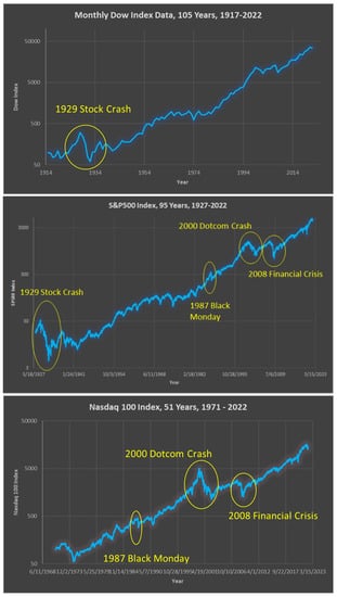
Figure 6.
A remarkable century of markets and growth, even through the Depression and World Wars: (top) 105 years of the Dow; (middle) 95 years of the S&P500; (bottom) 51 years of the Nasdaq index; data from (macrotrends 2022).
- Markets have long-term trends, generally up.
- They have periods of downturns as well, which can be protracted.
- They also have some rapid plunges.
- They may even have some self-similarity properties at different scales (a point we mention, but do not explore).
5.3. Simulation Setup
To make measurable progress, let us limit the scope of our inquiry to some investment specifics. We are interested in whether an individual small investor, starting with some initial capital, can possibly outperform a market index over the course of a lifetime of investing (say 40 years) or whether the investor can reduce her/his drawdowns over the same period while achieving similar gains. Either of these results is a win; both would be a home run. Rather than developing a strategy for value investing, we will simply perform market timing. To avoid picking stocks, we invest in a market index itself, but decide when to be in/out (or even inverse). To be specific, we focus on U.S, markets: the S&P500 (SPX) and the Nasdaq (IXIC) indices. In summary, we consider just the performance after 40 years of a single initial investment (say $1K), and ignore both inflation and taxes, but do include the cost of money (pegged at 3% interest), as well as slippage in making investment decisions (0.25%). Since inflation affects all investment strategies, it is fair to ignore it for comparison purposes (but we must remember that the multiples we achieve are unadjusted). Taxes are more serious, but if one manages these trades in a retirement account such as an IRA, then taxes can be ignored safely for now as well. In a period of 40 years, the investor is likely to come across many types of markets, and indeed, the last 40 years did see several major events (1987 Black Monday, 2000 Dotcom crash, 2008 financial crisis, 2020 Corona event). Therefore, a successful market timing strategy must, first and foremost, be able to negotiate such major events—by a strategy that, for every single day, decides to be in or out of the market, with nothing more than the daily closing market price up to that day only. (For simplicity, we restrict further to just daily closing price data and make decisions at most once a day, at the end of the trading day.) In particular, we must carefully avoid any lookahead bias in our work, since we will be dealing with time series for an entire stock or index history. We can add one further ingredient, in that we allow the investor to leverage up moderately (up to 2×) or even go inverse (up to −1× only) on the market. In the case of leveraging, we again include in our modeling the cost of money, herein modeled with a 3% interest rate (but revisit that later). Let us decide on a concrete end goal.
Simulation Setup: start with $1K, allow leverage, model interest rate as 3%, and track performance of a timing algorithm vs. an index (buy-and-hold) for decades.
Goal of market timing an index: to meet or exceed the market index, while reducing drawdowns (to <50%).
Such a strategy, if moreover easy to execute, would be a bonanza for the individual investor. It can also help professionals and be a profitable business model.
5.4. Market Performance Metrics
Before we begin our investigations, let us clarify some performance metrics. To simplify matters, we consider a single initial investment and track the trajectory of that value in an investment, over a period of time (investment period). The first and most important measure that is immediately comprehensible is a graph of the investment value over time, and this will be our primary evidence. If an investment A returns superior gains compared to investment B, then the graph of A would generally be above that of B and, other things being equal, would tend to be preferred. However, this simple idea can be further elaborated. If A experiences greater volatility (e.g., variability) than B over the investment period, then that would temper our interest in investment A vs. B. Of course, all investments experience volatility, and thus have some risks. One wants a measure of the risk-adjusted return of an investment to properly compare them. Finally, how much return one obtains from an investment should be compared to what the market may call a “risk-free” investment, e.g., the yield on a U.S. Treasury (bill, note, or bond), backed by the “full faith and credit of the US government”. These are debt instruments of the U.S. government, giving very modest yields, but with little to no risk, and are a common yardstick by which to measure performance. Thus, the so-called Sharpe ratio was developed, named after the 1990 Nobel Prize-winning economist William F. Sharpe (Sharpe 1994), which is just the excess return of an investment (over a risk-free one), divided by the volatility of the investment, measured as the standard deviation of the excess return, when measured in increments of time (for example, daily returns). In practice, the Sharpe ratio is computed using the expected value of the excess daily return of the asset, divided by the standard deviation of the daily return. In fact, many authors drop the risk-free part of this formula (setting it to zero), especially for short-term or intraday trading, and simplify it to just the normalized portfolio (or stock) return, normalized by the standard deviation.
Here, E means expectation value or mean over the data record, which may be for 10 days or 10,000. Since we want the Sharp ratio as an annualized measure, while the returns are measured here on a daily basis, the root N is used as a normalization factor (and would not be needed if returns were measured yearly). Finally, along with many other authors (including Theate and Ernst 2002), we simplify by setting the risk-free return to zero. Note the important use of the standard deviation, the root of the variance (or mean-squared error (MSE)), to normalize the risk-free return. A key and known problem with the use of the standard deviation in the Sharpe ratio is that it penalizes variability in the upside just as much as the downside, which contradicts investment objectives (a defect cured by the so-called Sortino ratio). For completeness, we also mention another useful measure, the Treynor ratio (Treynor and Mazuy 1966), whose numerator is the same as for the Sharpe ratio, but the denominator is the beta of the portfolio (defined as the ratio of a covariance to a variance ). A number of papers and blogs discuss the use of both the Sharpe and Treynor ratios (plus scaled versions), for example to measure hedge fund performance (van Dyck 2014). For now, we stay focused on the well-known Sharpe ratio, and another useful ratio we will introduce shortly.
It is in fact well known that the mean-squared error (MSE), or mathematically, the -norm, which derives from geometry, where it is a good distance measure, may not be the best measure in other unrelated fields in engineering and computer science (such as in image processing); so, it is inadequate in finance as well. The Sharpe ratio is in fact much touted in the professional literature, and investors are even advised (by investment advisors) that assets with Sharpe ratios in the range 1 to 2 are good, those in the range 2 to 3 are better, and those with 3+ are excellent. With 10K investment funds in the U.S. alone, some invariably find themselves with rarefied Sharpe scores, despite the fact that most of them underperform the market. However, in fact, these stellar ratings generally never hold up over a period of years or decades. It is a roll of the dice to find such highly rated investments at any given time. Thus, the game of chasing very high Sharpe-ratio-bearing investments can be illusory. The Sharpe ratio is not our favored yardstick for measuring meaningful performance, and we will rely on a simpler, more useful one. Later, we will be able to contrast them.
First, for clarity, in our discussion, we will mainly be interested in long-term investments, over a period of decades, so it is convenient to work with returns on an annualized basis. We will consider total return (also called gain) as a multiplicative factor on the initial investment. Due to the compounding effect of returns over time, we compute the following to obtain the annualized return. Note that an initial investment of dollars, with an annual rate of return r, over a period of M years, would give:
Finally, while volatility, as measured by the standard deviation of the daily returns, may be useful for professional investors and is based on underlying Gaussianity assumptions about daily returns, the reality is that such assumptions do not hold with real assets in the market, nor is the Sharpe ratio especially useful to the average long-term investor. What is truly meaningful to the small investor, who is investing for a lifetime, is measuring returns against major losses or drawdowns, especially the maximum drawdown over an investment period, which may be decades long. The reason for this is that the investor may need to withdraw her/his funds at an unknown time. While the statistical variability of an investment as measured by the Sharpe ratio is relevant to this, the maximum drawdown is much more critical, as it provides the greatest loss that the investor may suffer for getting out at a bad time. Mathematically speaking, we are more interested in the -norm of losses, rather than the -norm as measured by the standard deviation. For small investors with their life savings on the line, that is a much more meaningful measure. Thus, we introduce the simpler, but more valuable annualized return over maximum drawdown, called RoMaD (RoMad 2020); we invented it independently as a natural metric and called it the ARMD ratio (AnnR/MaxD ratio).
Investment objective: In our view, the objective of sound long-term investment is to maximize the annualized return and minimize the maximum drawdown over the period of investment; that is, optimize the RoMaD.
Note that since the max drawdown is a global indicator of the data record, we could also work with the total gain, by using gain/MaxD. However, in this case, since we can continue to enhance the gain without limit by leveraging, while the MaxD is capped at 1.0, this would skew our performance metric to lead us to unfavorable trading regimes. We could never afford a very high maximum drawdown, approaching 1.0, in reality. Normally, we prefer to work with maximum drawdowns below 50%, or 0.5. By working with the annualized return, we keep this metric within bounds. This makes it more suitable for regression testing when desired. While the small investor is not equipped to perform such analyses, at least this notion is more manageable for that investor, who then may be able to follow guidance based on this objective. Note that, just as with the Sharpe ratio, investors may be advised to seek investments with high RoMaD scores as measured annually (e.g., 2 or more). However, again, such high scores do not persist. The real question is: Can one develop a strategy that provides solid returns such as a market index, yet allows the investor to survive the major Black Swan events that arise.
5.5. Rule-Based Trading Using Moving Averages
One simple market timing approach is in fact well known in the industry and involves the use of the so-called weighted moving average, WMA(N), the weighted average price of a stock or index over the past N days. Starting from a given day, labeled Day 0, count backwards up to N − 1 days and average the price on those days, with weights.
As a special case, set
More precisely, the exponential moving average (EMA) is an infinite sum going back, where We will mainly use the SMA for our elementary analysis. Now, a very simple and well-known indicator based on the SMA is the following. Let S and L be two positive integers, S < L, and consider SMA(S) and SMA(L). For example, one can set S = 50 and L = 200 and consider the 50-day and 200-day simple moving averages. Our indicator is the difference.
Algorithm 1.
Ind = SMA(50) − SMA(200). If Ind > 0 be in, else be out.
Here, “in” means be long the market, while “out” can mean go to cash, or even sell short the market (for now, we just go to cash). Of course, while these specific time periods are widely studied in the market, there is nothing sacred about them. To get an idea of simple moving averages and what this algorithm entails, we present some graphs. In preparation, first note that there are approximately 250 trading days in a year (about 252.75), and it is easier to plot with just trading days as the x-axis. Therefore, 2500 trading days is approximately 10 years, and 10,000 trading days is about 40 years, roughly the investment horizon of a typical investor. Then, 25,000 trading days is approximately 100 years. Thus, out of convenience, our plots will frequently use trading days on the x-axis. In Figure 7 and Figure 8, we show the SPX for the last 94 years, with the unadjusted buy-and-hold (BnH) performance for the last 93 and 40 years, respectively, ending 1 April 2022.
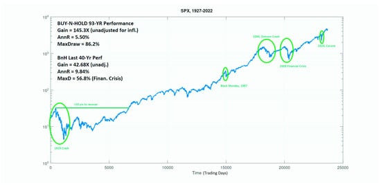
Figure 7.
S&P500 (SPX), 30 December 1927–1 April 2022, graphed for 94 years (tested 93+ years due to MAs). The market trends upwards, but it has many dips and valleys. The buy-and-hold (BnH) performance is given for the past 93 and 40 years. For convenience, the x-axis is now time in trading days.
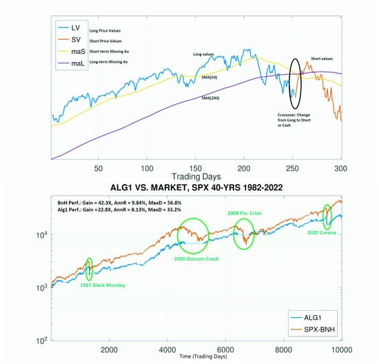
Figure 8.
(top) Example of Algorithm 1 in action, with a segment of the S&P500 data, showing key elements. When SMA(50) crosses below the SMA(200), the method switches from long to short or cash, and vice versa. (bottom) Performance of Alg1 vs. BnH, on SPX, 1982–2022. Alg1 underperforms simple BnH, but it reduces drawdowns. That in itself may be a benefit for small investors.
In our simulations, we invest $1000 just once in the beginning and track the performance of trading algorithms in both growing that amount, as well as in the drawdowns (or percent losses) along the way. Specifically, we measure the performance of trading algorithms using: (a) the raw, unadjusted gain as a multiplier on the initial principle (here, assumed to be $1000); (b) the annualized return as a percentage (e.g., a 10% return is a multiplier of 1.1×); the maximum drawdown as a percentage. The approach can be extended to include both periodic and irregular investments as well, but our streamlined simulations will be indicative. With these preliminaries, Figure 7 shows the performance of BnH on the SPX for 93 and 40 years, while Figure 8 shows the performance of our Algorithm 1 vs. BnH on the SPX for the past 40 years. It indicates that while Algorithm 1 fails to outperform BnH in this period, it does at least reduce drawdowns to more manageable levels (33% vs. 57%). Moreover, that drawdown protection seems to be consistent, even holding flat during the 2000 Dotcom and 2008 financial crises. However, note that the Black Swan events of October 1987 and the COVID-19 outbreak do trip up Algorithm 1, just as they do BnH. This is a problem to address for algorithmic trading. We remark that Algorithm 1 makes only 36 trades in the 40-year period, or about 1/yr. This method is already useful for many investors, whose risk tolerance may be limited. Of course, for some other investors, the loss of performance may be a non-starter.
For many small investors, though, controlling drawdowns would be a powerful benefit, especially for those approaching retirement. Note however that sudden Black Swan events such as Black Monday and the Corona pandemic are too rapid for this method to alleviate. However, we can also observe that such rapid events do not have significant repercussions over time on their own.
To make further progress, we need additional tools. For one, we can use a well-known technique, leveraging; that is, we borrow money on margin every day to buy more than our money can afford (paying interest daily, assumed here at 3% annualized, or just use leveraged funds) when we have a long signal, but revert to cash when we have a sell signal.
Algorithm 1.1.
Algorithm 1, but buy at 1.5× if Ind > 0, cash if Ind < 0.
Algorithm 1.2.
Algorithm 1, but buy at 2 × if Ind > 0, cash if Ind < 0.
More generally, we could leverage in either direction with any numerical multiplier (e.g., 2.5×, −1.3×). We show in Figure 9 that Algorithm 1.1 does indeed slightly outperform BnH and reduce drawdowns. However, again, our two steepest Black Swan events really impact the performance gains that would otherwise be possible with Algorithm 1.1 without them (we still eke out a gain, but not very exciting). This algorithm, being just a slight variation on Algorithm 1, also performs 36 trades in the 40 years. However, given some performance gains for Algorithm 1.1, we up the leveraging in Algorithm 1.2. As expected, it does raise the performance. However, we note that the Black Swans are also magnified. They need to be dealt with. We must find the bread crumbs they leave.
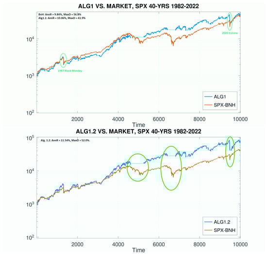
Figure 9.
Performance of variations on Algorithm 1: (top) Algorithm 1.1 with leverage = 1.5× and (bottom) Algorithm 1.2 with leverage = 2×. Note that as we leverage more, we can realize gains, but the Black Swan events are also magnified. Therefore, the desirable properties of increased gains and reduced drawdowns are a tradeoff, and Black Swan events are limiters.
5.6. Learning-Based Trading Strategies
With the decisive success of deep-learning-based methods in several key computer science applications (e.g., image recognition, natural language processing, and game playing), suddenly, every problem looks like a nail to the deep learning hammer. Financial trading is no exception. Since financial data are typically a time series (whether the adjusted daily closing of a security or the price every millisecond), any method that can predict the next sample or the direction of upcoming samples (trend) could be exploited by traders for financial gain. With this insight, a veritable flood of papers, books, blogs, and even YouTube videos purports to show you how to make money by using deep-learning-based prediction for trading; how well they work is another matter. Among books, we content ourselves with just citing (Jansen 2020). However, Peleg (2017) warns that, overwhelmed with data (not just the stock one wants to trade, but a world of possibly relevant data) and no reliable financial theory, “most models have poor predictive capabilities on financial data.” The tasks of figuring out what is relevant, what features to use, and how to make decisions are all challenging. In effect, one must learn what is relevant data, what conclusions to draw from them, and what actions to take in response, in order to obtain rewards (e.g., profits). Thus, in the recent literature, there is an emerging trend to use reinforcement learning (RL) to train an agent (often itself a neural network, thus deep RL (DRL)) to learn both features and trading decisions (strategies) on its own (Li 2018). There are many resources for DRL online, including a library of DRL algorithms ready to “spin up” at OpenAI.com (rlspin 2022).
A schematic of RL is given in Figure 10. An environment provides a time series of state and reward information at each time increment. The state may be a complicated structure (e.g., all the positions on a game board at a given time), while the reward is a numerical value taking on a real number (positive or negative). The objective of such a system is to maximize the reward over time. Processing that stream of incoming data, the agent determines a new action at each time increment and interacts with the environment with it, and the process continues. Based on the history of the rewards obtained, the agent learns to develop a “good” policy of action based on incoming state data, following a policy gradient to improve the reward over time. More precisely, at each time point, the agent wants to maximize the total reward, which is the sum of all rewards going forward, but where future rewards are discounted to obtain their present value, incrementing the discounting with time. For details, see (Li 2018). In the case of financial transactions, the incoming state can be simply the current stock price (but could include many other variables such as other stocks, technical indicators, interest rates, news, sentiment, etc.), and reward can be the gain/loss based on the previous action. The action itself is a buy, sell, or hold decision. From that collective time history, the agent learns to make decisions that optimize the total reward. We can see that in finance, there may be many variables that influence the stock price of interest that may be available, leading to a potentially massive overload of data. Thus, the state space in our model could becomes very complicated. We take the pedestrian point of view that we are only interested in one variable, the price of a given stock or fund, ignoring all other variables, and so, we track only a single time series.

Figure 10.
Schematic diagram of (deep) reinforcement learning. An environment (in our case, a stock market) provides a time series of the current state, as well as the current reward for the previous action. That data can be the next increment of the stock price, as well as reward information about the gain or loss due to the last action. In turn, an agent (especially a deep learning agent) processes that new incoming data of state and reward and, combined with the prior history, processes that information to determine a new action, by which it interacts with the environment (e.g., places a buy or sell order or holds shares). The agent is not provided any training data with prior optimal actions, so in that sense, this system is unsupervised. However, the system does provide a concrete reward for each action. Thus, RL stands as a separate branch of learning, distinct from both supervised and unsupervised learning. It has proven promising in many areas already.
In the deep RL version, the agent is essentially a neural network, for example a recurrent neural network, such as a long short-term memory (LSTM) network. DRL is an exciting development in AI. It has found many applications, including great success in beating the top human Go players (by AlphaGo). Its application in finance, though vigorously pursued, is still in its early stages, but seems promising. A number of papers have investigated the use of DRL, especially a method called Q-learning (Li 2018), for trading over relatively short periods of time (typically a few hundred trading days). Theate and Ernst (2002) presents a variant of Q-learning, applied to market timing to periods over a year, obtaining good results in their experiments. We tested that algorithm ourselves, on a much longer data record, with mixed results. Note that the performance of a DL method is statistical in nature, and that experiments should be repeated many times (e.g., 50 to 100) to obtain aggregate performance. This is not the case with deterministic rule-based algorithms.
Note that in learning-based applications, one needs both training data and separate testing data. In applications such as image recognition, where the various instances of an object can be regarded as independent, it is easy to randomly select a subset (typically 80%) for training and use the remaining 20% for testing. In timed data, such as financial time series, this approach is not directly applicable, due to the linearly ordered time structure. Instead, it is now common practice to use a start date, an end date, and a split date in between, where training occurs during [start, split − 1] and testing occurs during [split, end], where the testing period is typically much smaller than the training period. However, in our consideration, we are interested in investing over decades.
We took the long history of the SPX index and tested using the method of (Theate and Ernst 2002), and we found that the results were somewhat disappointing as it underperformed the index, but at least maintained moderate drawdowns despite the many Black Swan events; see Table 1. A more aggressive action approach in the model, including leveraging, could potentially yield a more usable strategy; we are novices in this method and used only default parameters. Finally, we note that to test on very long periods such as 40 years, one needs a more rigorously trained model, generally 4× the test length (e.g., 160 years). While the history of the SPX may be limited and does not afford 160 years (but we did note improved testing performance after longer training; see Table 1), there are many other indices in the U.S. and worldwide and tens of thousands of stocks and funds one can train on, not to mention many other relevant (or confounding?) variables one can include in the state space model. The pressing question is: What else can actually help? Does knowing the SPX up to a given date T help trade IXIC on T? How about AAPL, MSFT, FTSE, Fedfunds? How about Forex, news, Twitter? What optimal combination of additional variables to use in a trading model is currently an unsolved problem. We thus have a new Wild West frontier to explore. Fortunately, we do not need it to obtain good returns.

Table 1.
Performance of the TDQN deep RL algorithm, on long-term investing, using the SPX index. In this simulation, we trained on 20 years of data (1960–1980) and tested on 42 years (1980–2022), with quite modest results. In a second simulation, we trained on 40 years (1940–1980) and tested on 42 years (1980–2022), with slightly better results. The RL method, in our limited testing, obtained modest performance, but reduced drawdowns significantly. With the longer training period, the Sharpe ratio improved. The SPX itself had a Sharpe ratio of 0.586 in the test period. Note that the risk-free rate was set to zero in computing the Sharpe ratio.
5.7. Back to Basics—Rule-Based Approaches
At this point, while the DRL approach appears promising, with our disappointing initial results, we return to our elementary framework of rule-based approaches, generalizing the simple moving average methods. We first mention that leverage can be applied in both the long and short directions and that one is free to develop more sophisticated indicators based on moving-average-type filters on the price history, for example using three or more moving averages (MAs) (we used up to four MAs), to develop a kind of algebra of rules to create trading indicators. These algorithmic methods are fixed functions, require no training, and thus can be tested on full data records. We developed a suite of twenty core algorithms, which, together with about 7–8 parameters to set, constitute a large library of over 1K distinct algorithms that we regress over (but hold constant during an entire test).
We call our approach FastHedge, which includes both fast growth due to leverage (typically under 2×), as well as hedging by going inverse the underlying when needed. To simplify matters, we only used actual leveraging in the positive direction in our simulations. Even with this large library, since there is no learning, our sims compute in seconds for a 40-year data record, even on a laptop. However, importantly, these elementary methods can still be effective. We now show what is possible with this machinery. For the SPX, we present results for an algorithm called Alg2 from the library, which definitively improves on BnH on SPX. For Nasdaq (IXIC), we present results for a method called Alg3, which in fact provides excellent results (Figure 11). Both of these provide superior performance, while still constraining drawdowns to some extent, with Alg3 on Nasdaq especially noteworthy. Moreover, these performance gains are consistent across the time periods, negotiating both major market crashes and the special Black Swan events. While these Black Swan events continue to be challenging, their impact has been partly controlled while still obtaining excellent gains in Alg2, and much more so in Alg3. In fact, Alg3 explicitly overcomes the 1987 Black Monday and actually benefits from the 2000 Dotcom crash, which is remarkable. These strong results indicate that this method is applicable to both professional and individual investors for long-term investment performance. In turn, these high performance levels also suggest that major Black Swan events often have some kind of tell-tale early markers that our algorithms are subtly picking up on.
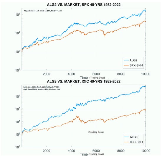
Figure 11.
Performance of more sophisticated algorithms on SPX and IXIC, still based on the same set of ideas, which deliver strong performance, yet limited and improving drawdowns. Since these time periods include several major market events, including the Black Swans, these results indicate that fairly elementary algorithms can indeed deliver powerful investment results, which may be applicable to both professional and individual small investors.
6. Surviving Black Swans and Interest Rates
We already showed that one can obtain good results with our framework, at least on major indices such as the SPX and IXIC. However, one possible limitation is that while we assumed that the cost of money was accounted for in our model, it was set at just 3% annualized. While suitable for the last decade, it is no longer appropriate going forward. In fact, while we are in a period of historically low interest rates for the past 15 years, past rates have often been much higher, and so may futures ones be; see Figure 12. To get a handle on interest rates, we will plot the well-known federal funds rate. What is more, one may assume that actual margin interest rates for a portfolio are on the order of one percent above the federal funds rate. Note that our era of low interest rates may once again be changing to higher ones.
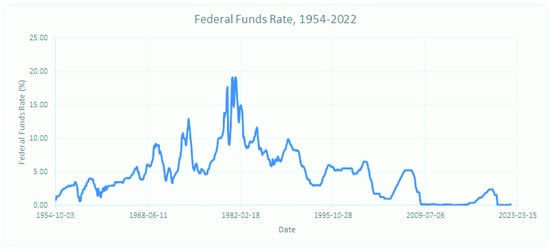
Figure 12.
The historical record of federal funds rate. Actual margin rates may be about one percent higher. Data: (ffunds 2022). For nearly 15 years, we have been living in an era of low interest rates. That now appears to be changing.
With this serious reality, a first reaction is to develop a method that avoids leveraging altogether, making it impervious to interest rate fluctuations. Figure 13 presents our key simulation result, without leveraging, which obtains gains, successfully negotiates all the well-known Black Swan events, and even profits from them, providing a remarkably smooth growth pattern. It thus constitutes our strongest evidence that market timing can indeed be successful and applicable to individuals and institutions alike.
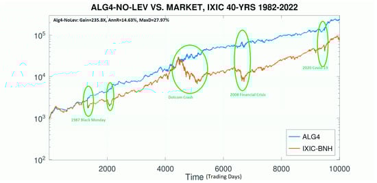
Figure 13.
Performance of an algorithm without leveraging, showing valuable gains, as well as markedly reduced drawdowns. Such an approach is immune to interest rate fluctuations and represents our strongest case yet on the utility of sensible market timing. Notice that we actually profit from the 1987 Black Monday and COVID-19 events!
However, let us see if we can push our luck further. In the next two graphs (Figure 14), we assume that the margin interest rate is 5% and 10%, respectively, and still use some leveraging. One would suppose that high margin rates would destroy our gains. They certainly dampen the returns, but do not destroy them. These methods execute about 15 trades/year, so leveraging is not performed continuously and does not incur the level of punishing penalties as one might otherwise expect. In sum, we can obtain excellent growth and tightly control losses. This is evidence that market timing, even with simple algorithms, can be effective.
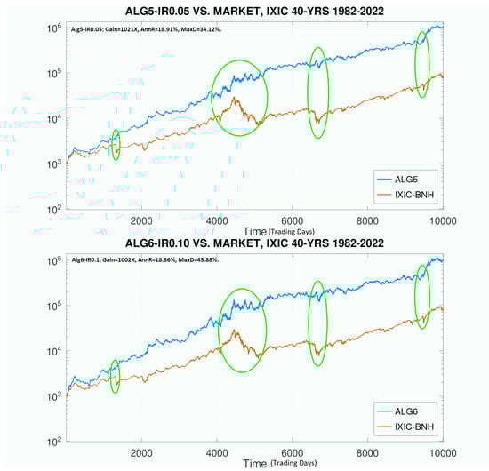
Figure 14.
Results using some leveraging, with margin interest rates of 5%, and 10%, respectively. Even then, we are afforded strong performance, and reduced drawdowns, although clearly, there is a penalty due to the cost of money.
7. Stock Trading
While our main interest is in trading major U.S. market indices such as the SPX and IXIC, we also tried our hand at trading individual stocks, including the well-known AAPL, MSFT, NFLX, and TSLA stocks that many other authors have tested, for comparison; see Figure 15. We applied the same FastHedge architecture with the same settings on these stocks. We obtained the following results. In this case, we made no effort to find the best performance, only some exemplary good results, to indicate that the method indeed applies broadly to stocks as well. (So far, Forex trading seems more challenging for our method, which is to be investigated.) From the graphs, we note that while AAPL and NFLX are profitably tradable, it seems that MSFT and TSLA are much less so, where good results are not very different from the underlying. MSFT had a truly spectacular 36-year run, and it seems it can hardly be improved by our methods (without magnifying the max drawdown unacceptably). Likewise, the meteoric rise of TSLA can still be improved a bit, while clipping some of its drawdowns. Note that as we are using a log scale on the y-axis, even small gains are quite significant.
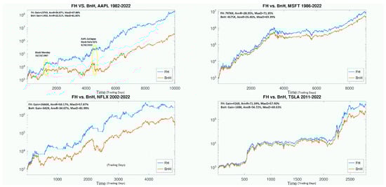
Figure 15.
Performance of the FastHedge suite of algorithms on some popular stocks, AAPL, MSFT, NFLX, and TSLA, for available periods of time, showing that even the best of them can be improved, but some only moderately.
8. Performance Summary
In this section, we collect some key results in tabular form, on our main indices SPX and IXIC, as well as the stocks just reviewed. This will provide a summary of our results in tabular form. The careful observer may notice some slight changes in results presented in earlier figures and those here. That slight discrepancy is due to the results being calculated just days apart. The simulations’ results are for the number of trading days listed in Table 2, ending on 22 April 2022. In conclusion, a trading decision platform called FastHedge was developed, encompassing a versatile array of trading algorithms, which permits effective trading on both U.S. market indices such as the SPX and IXIC, as well as some commonly traded stocks, such as AAPL, MSFT, NFLX, and TSLA; see Table 2. In almost every case, the leveraged FastHedge approach is able to improve annualized returns, as well as reduce drawdowns, to achieve improvements in total performance. Performance is measured by several metrics, including annualized return (AnnR), maximum drawdown (MaxD), the Sharpe ratio, as well as the annualized return over maximum drawdown (RoMaD), a ratio we developed independently and called ARMD.
Table 2.
Summary of key results of this paper in tabular form. A trading suite called FastHedge was developed, encompassing a large number of rule-based algorithms, which shows versatility in application to indices, as well as individual stocks, to provide strong performance, as well as reduced drawdowns, significantly reducing the effect of Black Swan events, a key design goal of the project. FastHedge models are generally leveraged. The simulations in the table end on 22 April 2022.
Note that the one exception is for MSFT, where the AnnR improved, but the MaxD became slightly worse. Yet, while the Sharpe ratio suggests a performance loss, the RoMaD suggests a slight performance gain. For well-heeled investors that can tolerate a 69% MaxD, a slight increase to 71% MaxD for a two-point gain in AnnR over 36 years would appear favorable. Looking at Figure 15, though the difference appears marginal, most investors would take the upper plot. More telling is the total gain (8Kx vs. 4.7Kx). It is our assertion that while the well-known Sharpe ratio may be useful for professional investors with relatively short-term trading horizons, for the individual small investor with a long-term investment horizon, our preferred measure RoMaD is more directly useful. Fortunately, our FastHedge platform is designed specifically to help the small investor achieve strong returns, yet survive the major Black Swan events that are their bane. Note carefully that our strong performance on the market indices SPX and IXIC, sustained over a 40-year investment period, were achieved with maximum drawdowns of under 50%, less than the 2008-9 financial crisis for example, which is something that can be recommendable to the small investor. Additional results, including the performance of FastHedge for 93 years of the SPX, are at https://fastvdo.com/fast-hedge.html (access on 30 April 2022).
9. Conclusions
We have now answered what we set out asking: the small investor can achieve good long-term returns, matching or exceeding market indices, while at the same time reducing drawdowns to more manageable levels. In the process, such an investor would achieve returns better than most of the funds in the marketplace.
In this investigation, we employed an elementary form of algorithmic trading, namely rule-based market timing, to achieve strong results in index investing over long periods. We were specifically cognizant of the risk of over-tuning to past market behavior in our algorithm development efforts (what is also called over-fitting or data-mining bias), a risk common to all algorithmic trading, since algorithms over-fitted to the past record may not respond well to novel market behavior in the future. With that in mind, we aimed to incorporate as few tunable parameters as possible, as well as to test specific fixed algorithms (including any parameters) on a variety of time scales, from 100 trading days up to 93 years, to check if they perform well in all types of markets. We found that single, specific algorithms can indeed perform consistently well for a particular variable (say the SPX or IXIC), over a variety of time scales. While a globally (in time) best algorithm may not be the best in smaller segments of time, it can at least provide acceptable performance in all time segments and provide consistently strong results in any extended time period ranging into decades.
While backtesting on past data records cannot fully predict future performance, these results suggest that our trend-following methods should generalize to unknown and novel future market movements, as long as major trends continue to persist. One clear direction for further research, already begun, is to test and improve the robustness of our FastHedge suite of algorithms using Monte Carlo simulations of future price movements. A second direction for further research is to test on arbitrary start and stop dates (our current tests were up to the present to obtain long time frames), test more variables, and incorporate other performance measures such as the Treynor ratio. Furthermore, one known failure mode of any moving-average-based trading algorithm is a market that oscillates around a decision boundary. While such events are not common in the data records, they do occur. Such event detection and amelioration methods can be incorporated into the suite in further work to make it more robust. Finally, we have not yet considered other financial markets (e.g., Europe, Asia) or Forex, etc., which would be natural extensions of our work. In the end, any trading algorithm can be improved or, alternately, also defeated by a well-contrived time series (sometimes called corner cases) designed to test its failure modes. The question is not whether real markets will test such corner cases (they will), but whether they will persist in them.
Our methods are suitable for guiding trading decisions by both individuals and professionals, are fairly easy to execute by hand and instantly in software, and show resilient performance in the face of the many Black Swan events in the past. While past performance is no guarantee of future returns and any algorithm can be improved, since the algorithms themselves are generic, as long as markets continue to have long-term trends, and mostly upwards, these methods should remain applicable. If real markets were totally random, no algorithm could consistently perform well. Real markets do have random components, but in the long run, they have trends that dominate. That trend is founded on overall economic growth. As we enter the era of climate change and the consequent effects on economies and markets, no one can predict future trends accurately, and continued economic growth is not guaranteed. Our only requirement is that there are and will be trends.
Author Contributions
This paper is principally the work of P.T., including all aspects of conceptualization, formal analysis, investigation, data acquisition and curation, and writing. W.D. assisted in carrying out some of the software simulations, primarily the deep reinforcement learning method, as well as in reviewing the drafted paper. All authors have read and agreed to the published version of the manuscript.
Funding
This research received no external funding.
Institutional Review Board Statement
Not applicable.
Informed Consent Statement
Not applicable.
Data Availability Statement
All data sources for figures other than our results are cited in the paper. Our own results figures rely on index and stock data widely available from many sources, for example historical data from finance.yahoo.com (access on 30 April 2022).
Acknowledgments
Special thanks to Richard Diehl for reviewing the draft paper as well as the simulation software.
Conflicts of Interest
The authors declare no conflict of interest.
References
- Anspatch, Dana. 2021. Why Average Investors Earn Below Average Market Returns. The Balance Blog. Available online: https://www.thebalance.com/why-average-investors-earn-below-average-market-returns-2388519 (accessed on 30 April 2022).
- Butler, Steve. 2015. The New Dark Art of Timing the Stock Market. USA Today, February 11. [Google Scholar]
- Chen, Ernest P. 2009. Quantitative Trading: How to Build Your Own Algorithmic Trading Business. Hoboken: J. Wiley. [Google Scholar]
- Chen, James. 2020. Available online: https://www.investopedia.com/terms/r/return-over-maximum-drawdown-romad.asp (accessed on 30 April 2022).
- Chen, Yong, and Bing Liang. 2007. Do Market Timing Hedge Funds Time the Market? Journal of Financial and Quantitative Analysis 42: 827–56. [Google Scholar] [CrossRef] [Green Version]
- Chien, YiLi. 2014. Chasing Returns Has a High Cost for Investors. St. Louis Fed Blog. Available online: https://www.stlouisfed.org/on-the-economy/2014/april/chasing-returns-has-a-high-cost-for-investors (accessed on 30 April 2022).
- Coleman, Murray. 2022. SPIVA: 2021 Year-End Active vs. Passive Scorecard. Index Fund Advisors. March 28. Available online: https://www.ifa.com/articles/despite-brief-reprieve-2018-spiva-report-reveals-active-funds-fail-dent-indexing-lead-works/ (accessed on 30 April 2022).
- Damodaram, Aswath. n.d. Dreaming the Impossible Dream? Market Timing. NYU Stern School of Business Document. Available online: https://pages.stern.nyu.edu/~adamodar/pdfiles/invphiloh/mkttiming.pdf (accessed on 30 April 2022).
- Estrada, Javier. 2008. Black Swans and Market Timing: How Not to Generate Alpha. Preprint. Available online: https://blog.iese.edu/jestrada/files/2012/06/BlackSwans.pdf (accessed on 30 April 2022).
- ffunds. 2022. Available online: https://fred.stlouisfed.org/series/FEDFUNDS (accessed on 30 April 2022).
- Fidelity. 2021. Fidelity Viewpoints. Why Work with a Financial Advisor. Fidelity Investments. November 1. Available online: https://www.fidelity.com/viewpoints/investing-ideas/financial-advisor-cost (accessed on 30 April 2022).
- Graham, John, and Campbell Harvey. 1994. Market timing ability and volatility implied in investment newsletters’ asset allocation recommendations. Journal of Financial Economics 42: 397–421. [Google Scholar] [CrossRef] [Green Version]
- Halls-Moore, Mchael. 2010. Successful Algorithmic Trading. Available online: https://raw.githubusercontent.com/englianhu/binary.com-interview-question/fcad2844d7f10c486f3601af9932f49973548e4b/reference/Successful%20Algorithmic%20Trading.pdf (accessed on 30 April 2022).
- Henriksson, Roy, and Robert Merton. 1981. On Market Timing and Investment Performance. II: Statistical Procedures for Evaluating Forecasting Skills. Working Paper. Cambridge, MA: Sloane School of Management, MIT. [Google Scholar]
- Investment Company Institute. 2021. Investment Fact Book 2021. Available online: https://www.icifactbook.org/21-fb-ch7.html (accessed on 30 April 2022).
- Investment Company Institute. n.d. Available online: https://icifactbook.org/21_fb_ch3.html (accessed on 30 April 2022).
- Jansen, Stefan. 2020. Machine Learning for Algorithmic Trading. Birmingham: Packt Publishing, July. [Google Scholar]
- Li, Yuxi. 2018. Deep Reinforcement Learning: An Overview. arXiv arXiv:1701.07274. [Google Scholar]
- macrotrends. 2022. Available online: https://www.macrotrends.net (accessed on 30 April 2022).
- Merton, Robert. 1981. On Market Timing and Investment Performance. I. An Equilibrium Theory of Value for Market Forecasts. Journal of Business 54: 363–406. [Google Scholar] [CrossRef] [Green Version]
- Pan, Eddie. 2022. Five Stocks to Watch that Institutions Are Buying Right Now. Blog. Available online: https://www.yahoo.com/video/5-stocks-watch-institutions-buying-213929921.html (accessed on 30 April 2022).
- Peleg, Yam. 2017. Trading Using Deep Learning. GPU Technology Conference. Available online: https://on-demand.gputechconf.com/gtc-il/2017/presentation/sil7121-yam-peleg-deep-learning-for-high-frequency-trading%20(2).pdf (accessed on 30 April 2022).
- Peters, Katelyn. 2021. Market Timing. Online Blog at Investopedia. Available online: https://www.investopedia.com/terms/m/markettiming.asp (accessed on 30 April 2022).
- Richards, Carl. 2014. Forget Market Timing, and Stick to a Balanced Fund. New York Times. January 27. Available online: https://www.nytimes.com/2014/01/28/your-money/forget-market-timing-and-stick-to-a-balanced-fund.html (accessed on 30 April 2022).
- rlspin. 2022. Available online: https://spinningup.openai.com/en/latest/index.html (accessed on 30 April 2022).
- Roberts, Lance. 2017. Opinion: Americans Are Still Terrible at Investing, Study Shows again. MarketWatch Blog. October 21. Available online: https://www.marketwatch.com/story/americans-are-still-terrible-at-investing-annual-study-once-again-shows-2017-10-19 (accessed on 30 April 2022).
- Ro, Sam. 2013. Chart of the Day: Proof That You Stink at Investing. Business Insider Blog. Available online: https://www.businessinsider.com/chart-proof-that-you-stink-at-investing-2013-3 (accessed on 30 April 2022).
- Seth, Shobith. 2022. Basics of Algorithmic Trading: Concepts and Examples. Investopedia Blog. Available online: https://www.investopedia.com/articles/active-trading/101014/basics-algorithmic-trading-concepts-and-examples.asp (accessed on 30 April 2022).
- Shadmehry, Cameron. 2021. How Profitable is Algorithmic Trading in 2021. Available online: https://medium.com/automated-trading/how-profitable-is-algorithmic-trading-in-2021-1b63489cd70a (accessed on 30 April 2022).
- Sharpe, William. 1975. Likely Gains from Market Timing. Financial Analysts Journal 31: 60–69. [Google Scholar] [CrossRef]
- Sharpe, William. 1994. The Sharpe ratio. The Journal of Portfolio Management 21: 49–58. [Google Scholar] [CrossRef]
- Shen, Pu. 2002. Market Timing Strategies That Worked. Working Paper 02-01. Federal Reserve Bank of Kansas City, May. Available online: https://www.personalfinancelab.com/wp-content/uploads/2013/03/RWP02-01.pdf (accessed on 30 April 2022).
- Sullivan, Ryan, Allan Timmermann, and Halbert White. 1999. Data-snooping, technical trading rule performance, and the bootstrap. Journal of Finance 245: 1647–91. [Google Scholar] [CrossRef]
- Theate, Thibaut, and Damien Ernst. 2002. An Application of Deep Reinforcement Learning to Algorithmic Trading. Available online: https://arxiv.org/abs/2004.06627 (accessed on 30 April 2022).
- Treynor, Jack, and Kay Mazuy. 1966. Can Mutual Funds Outguess the Market? Harvard Business Review 44: 131–36. [Google Scholar]
- Van Dyk, Francois, Gary Van Vuuren, and Andre Heymans. 2014. Hedge Fund Performance Using Scaled Sharpe and Treynor Measures. International Journal of Economics and Business Research 13: 1261–300. [Google Scholar] [CrossRef]
- Vanguard Research. 2019. Putting a Value on our Value: Quantifying Vanguard Advisor’s Alpha. Vanguard. February. Available online: https://www.vanguard.com/pdf/ISGQVAA.pdf (accessed on 30 April 2022).
- Zakamulin, Valeriy. 2014. The Real-Life Performance of Moving Average and Time-Series Momentum Rules. Journal of Asset Management 15: 261–78. [Google Scholar] [CrossRef]
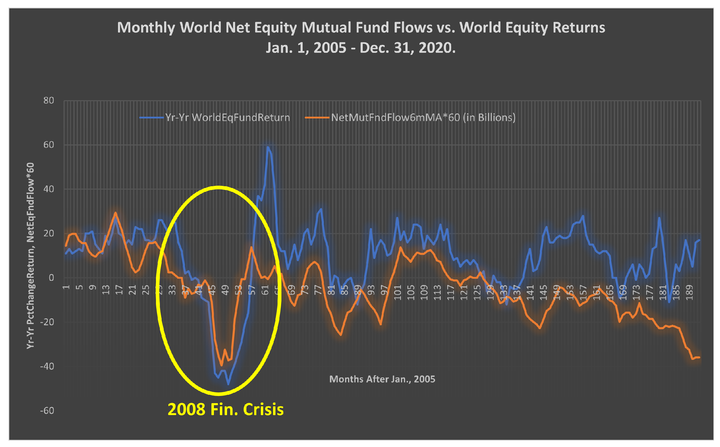
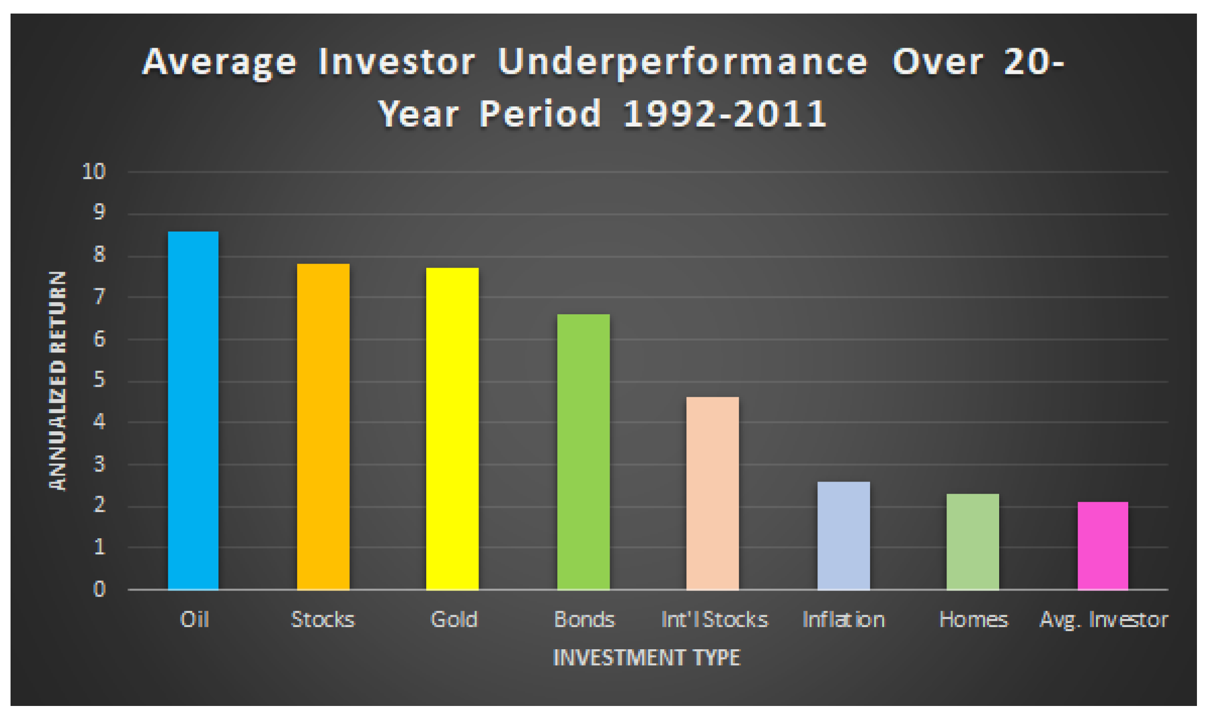
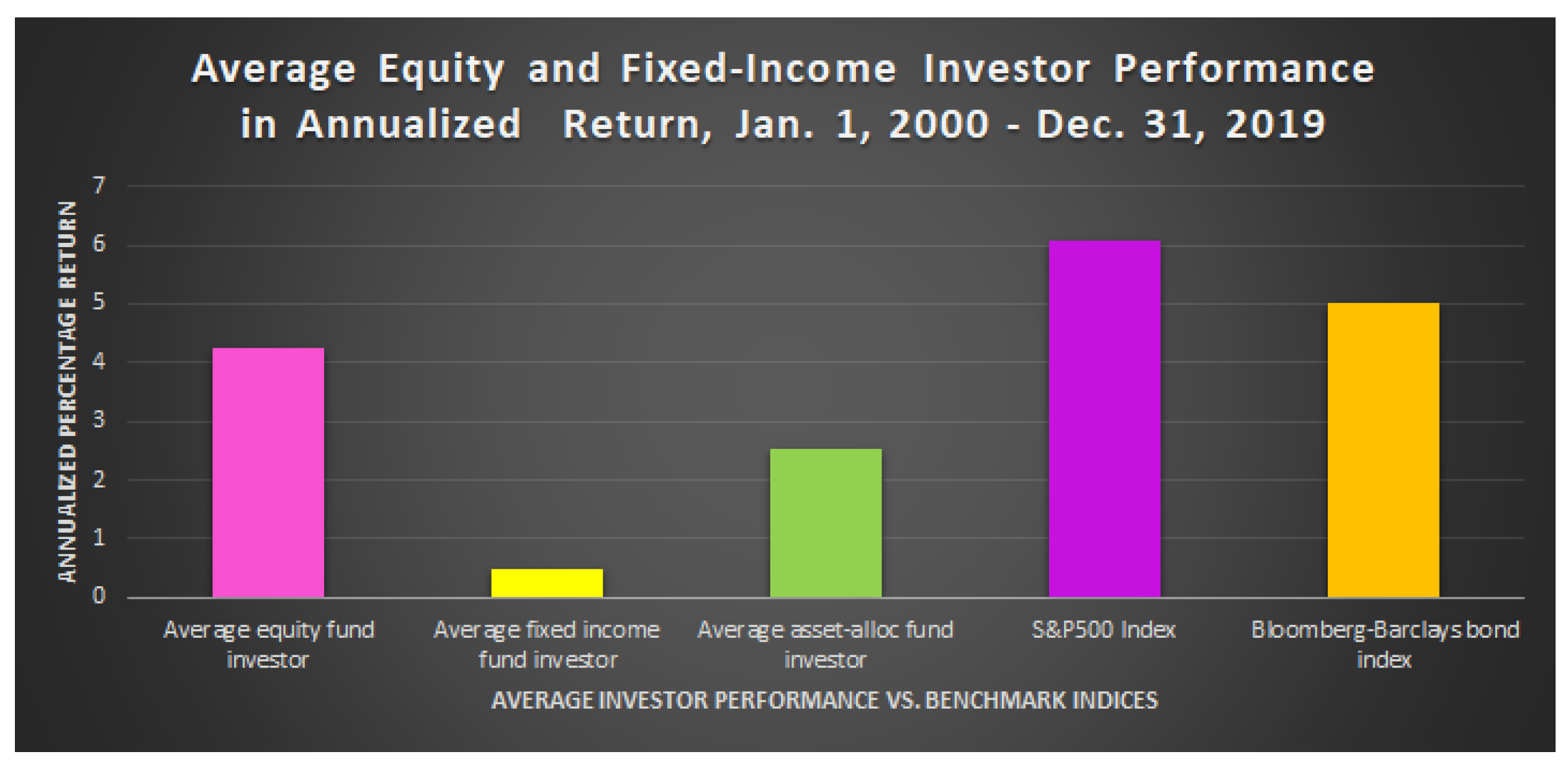

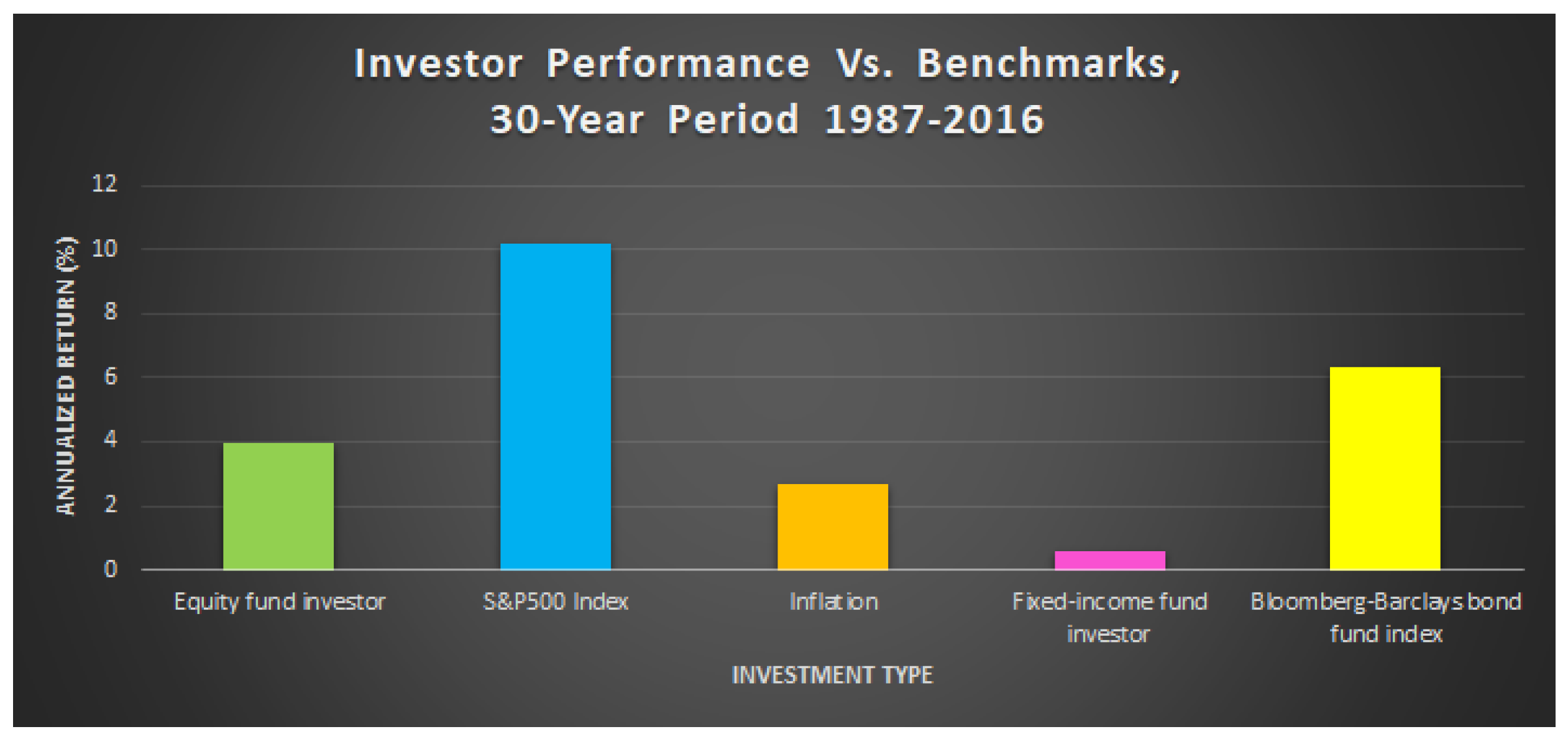
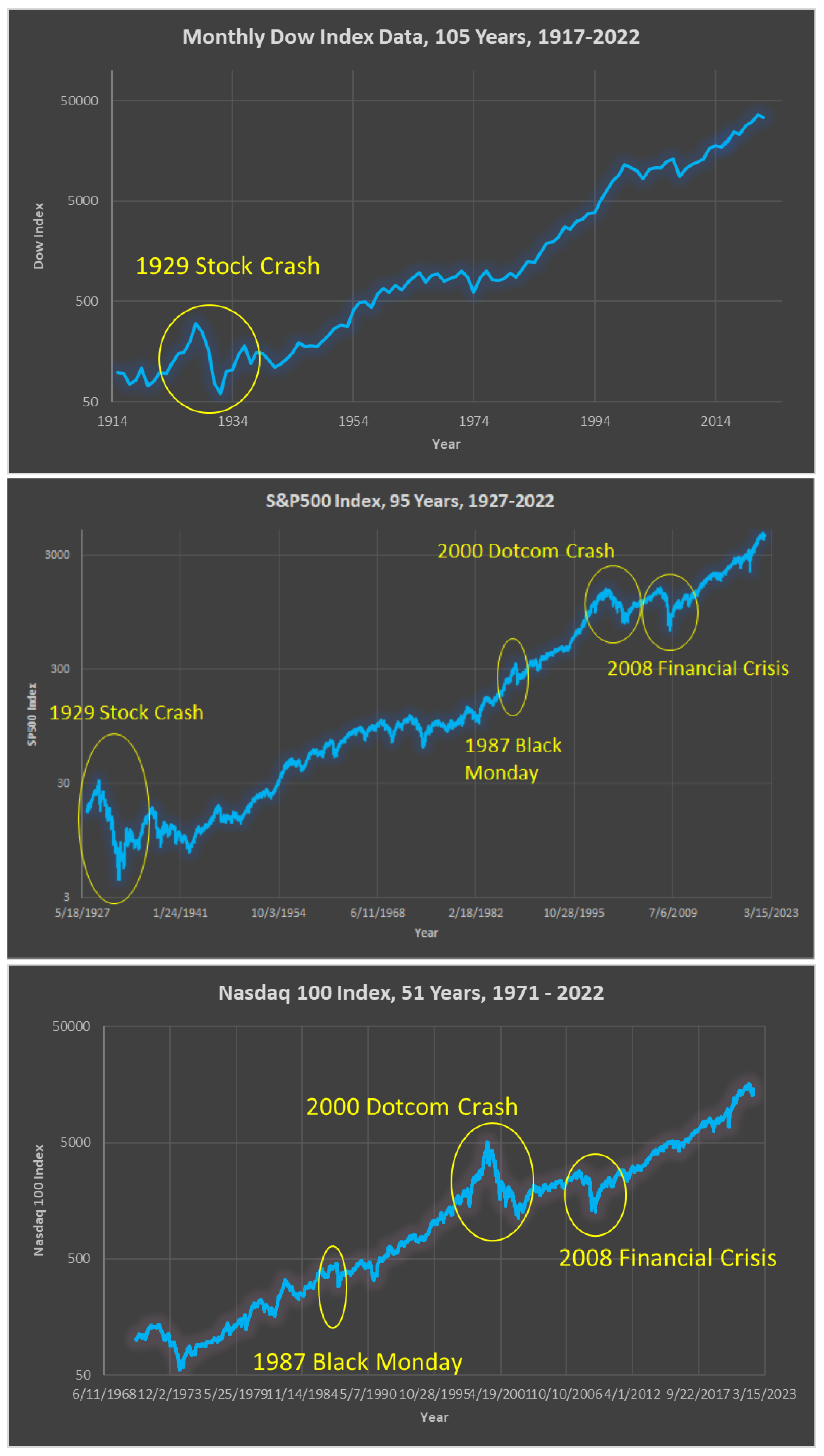
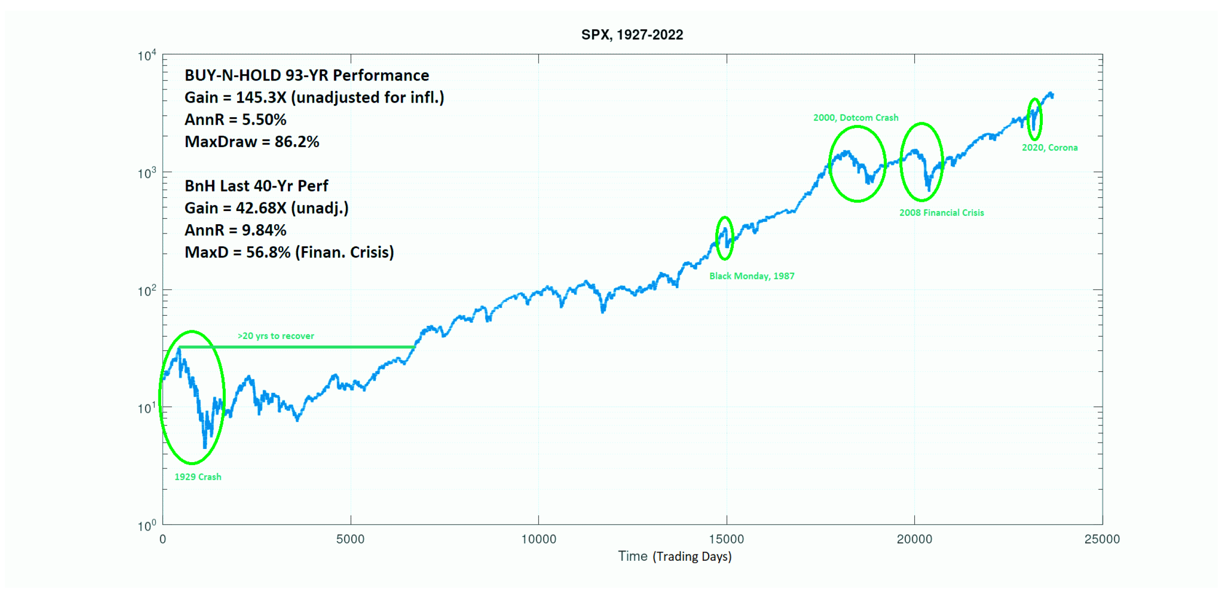
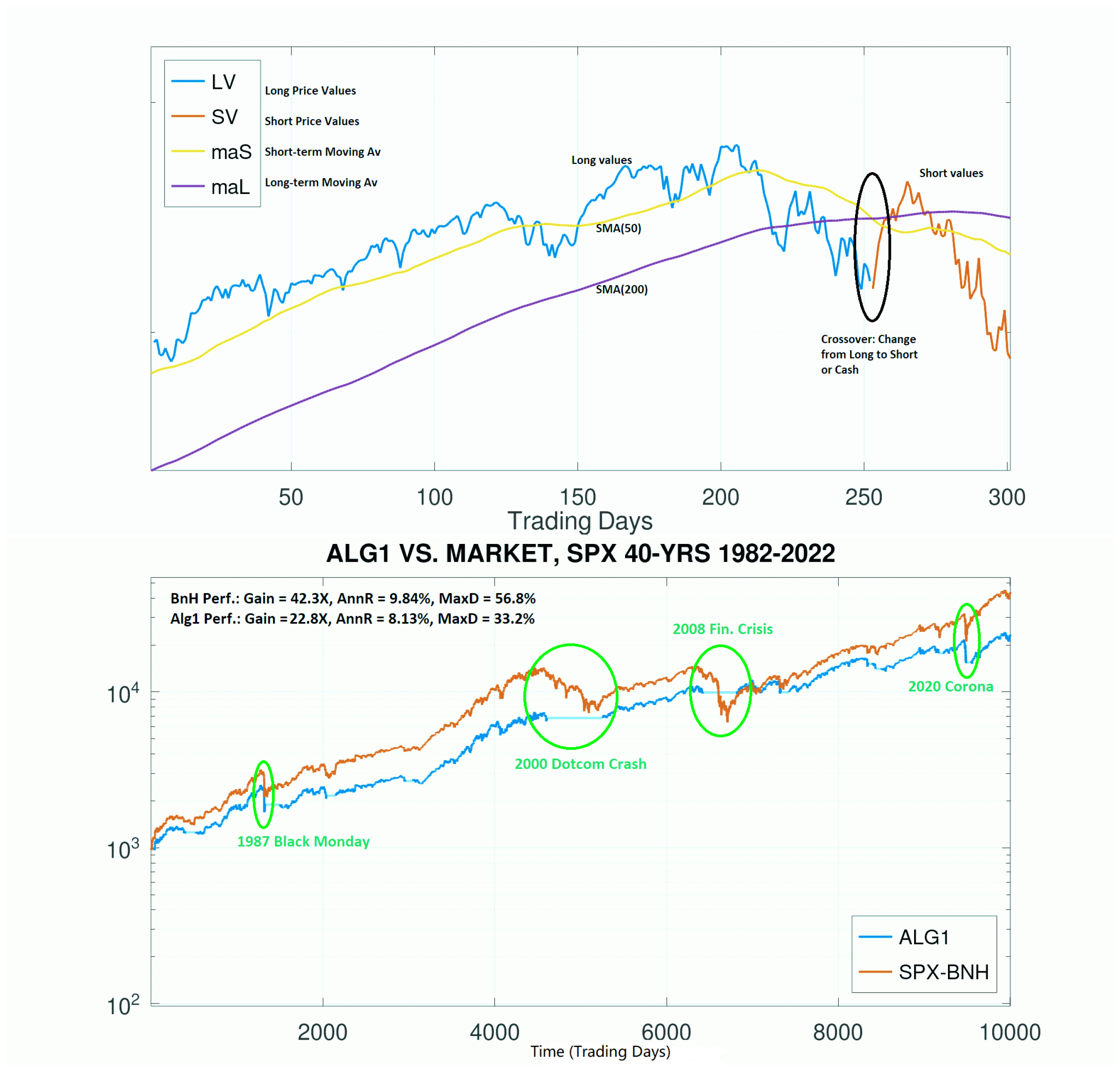
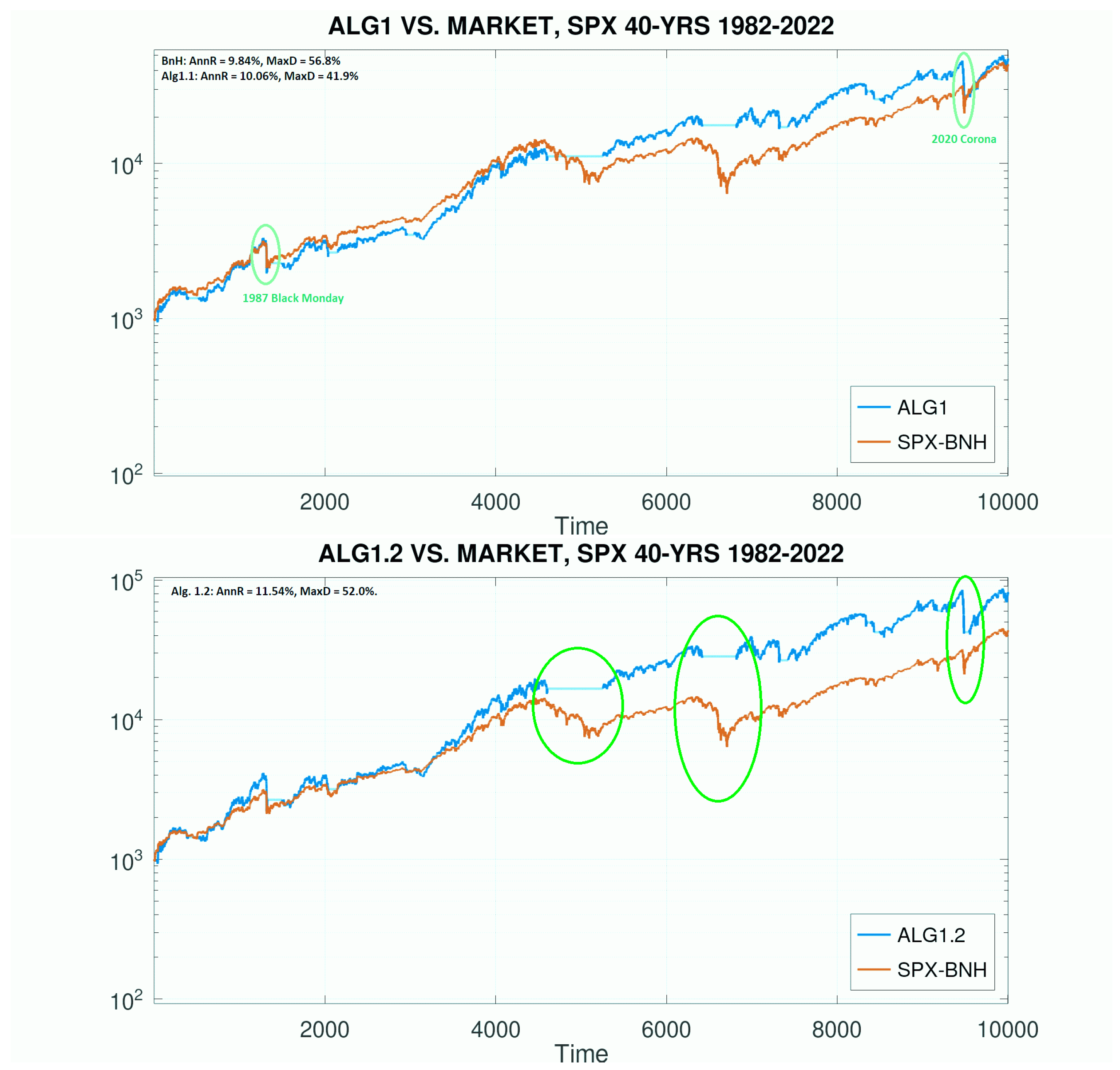
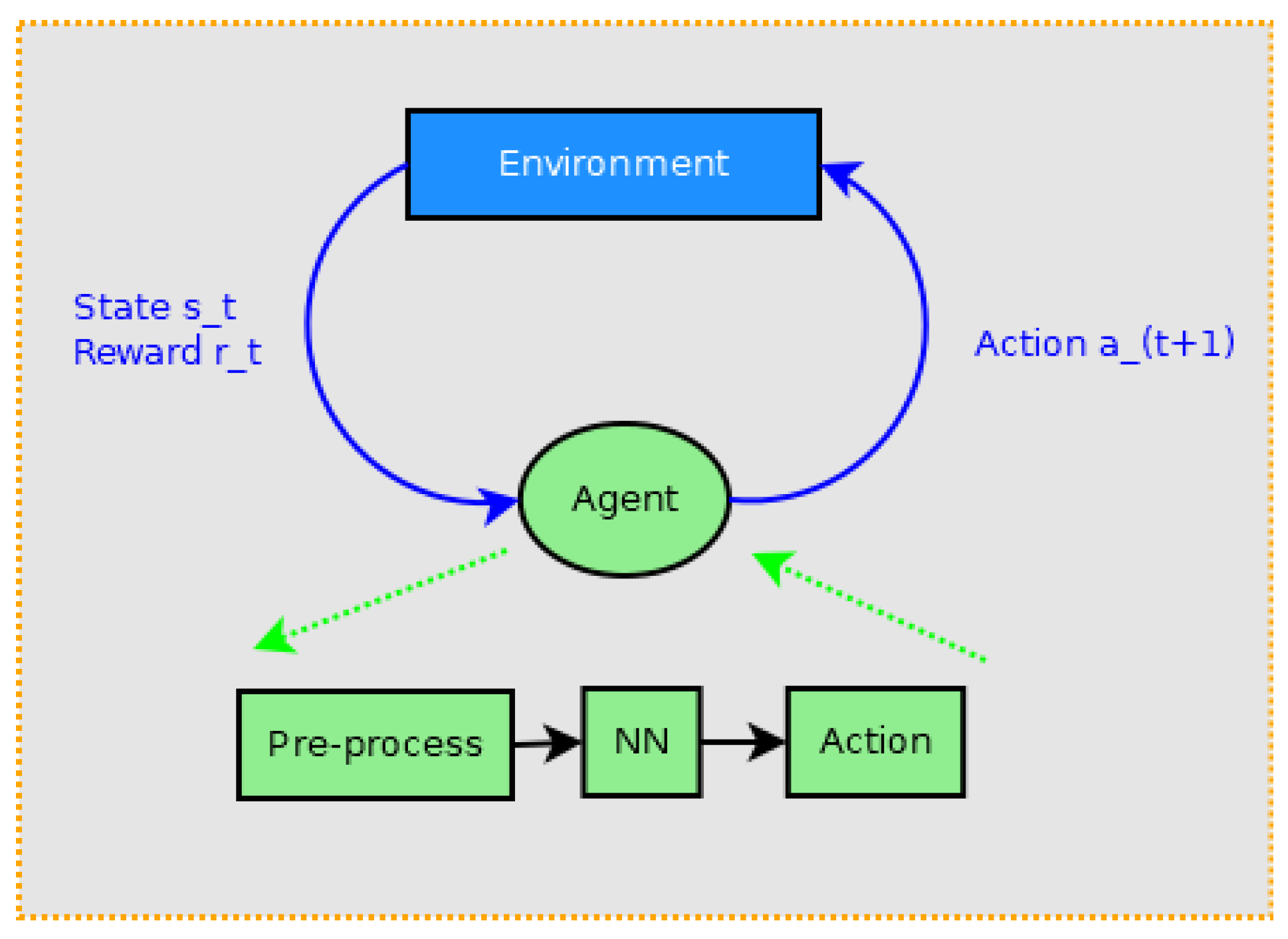
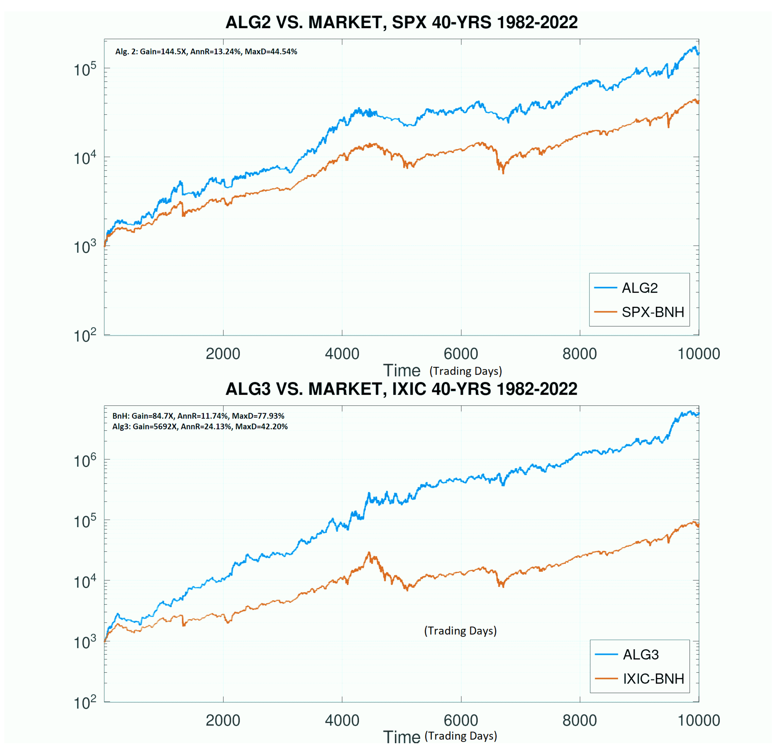
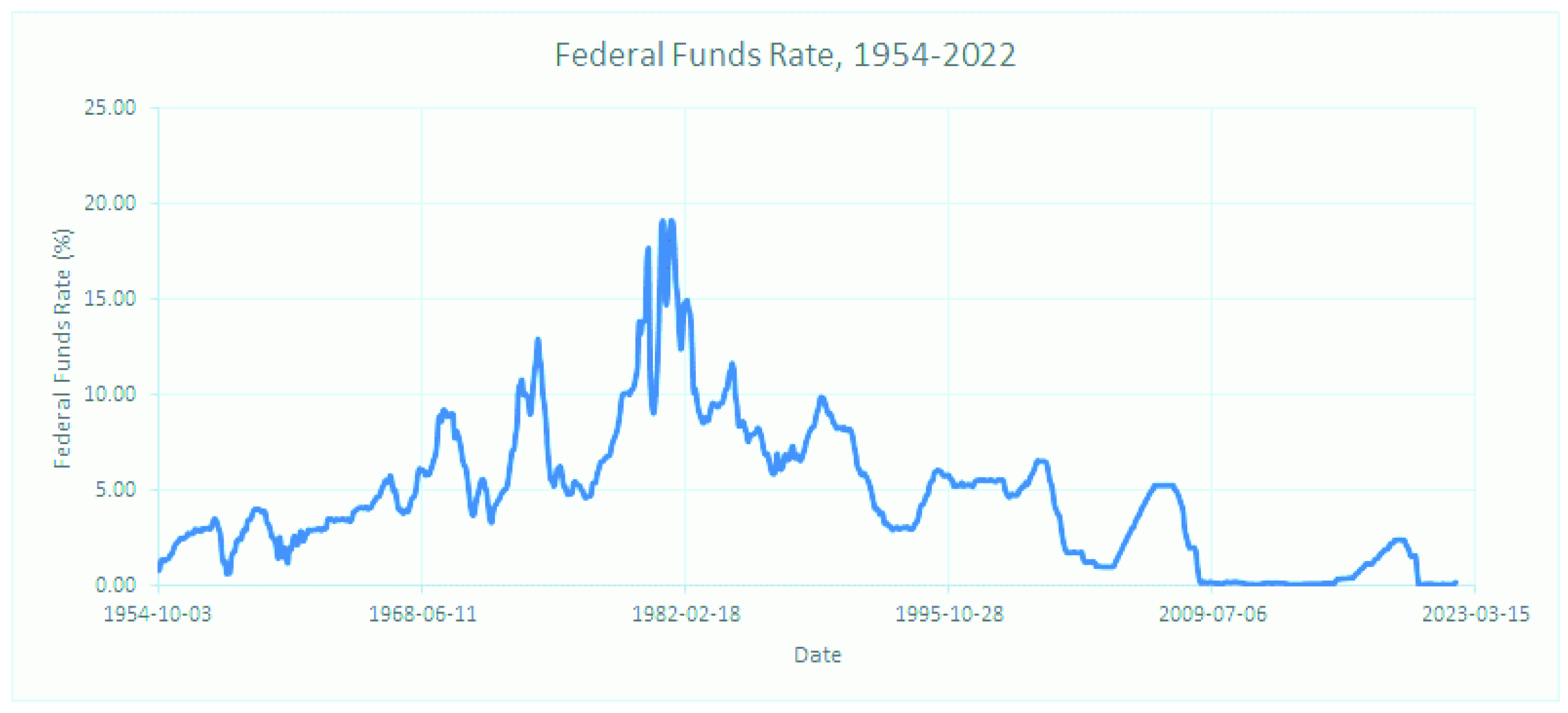
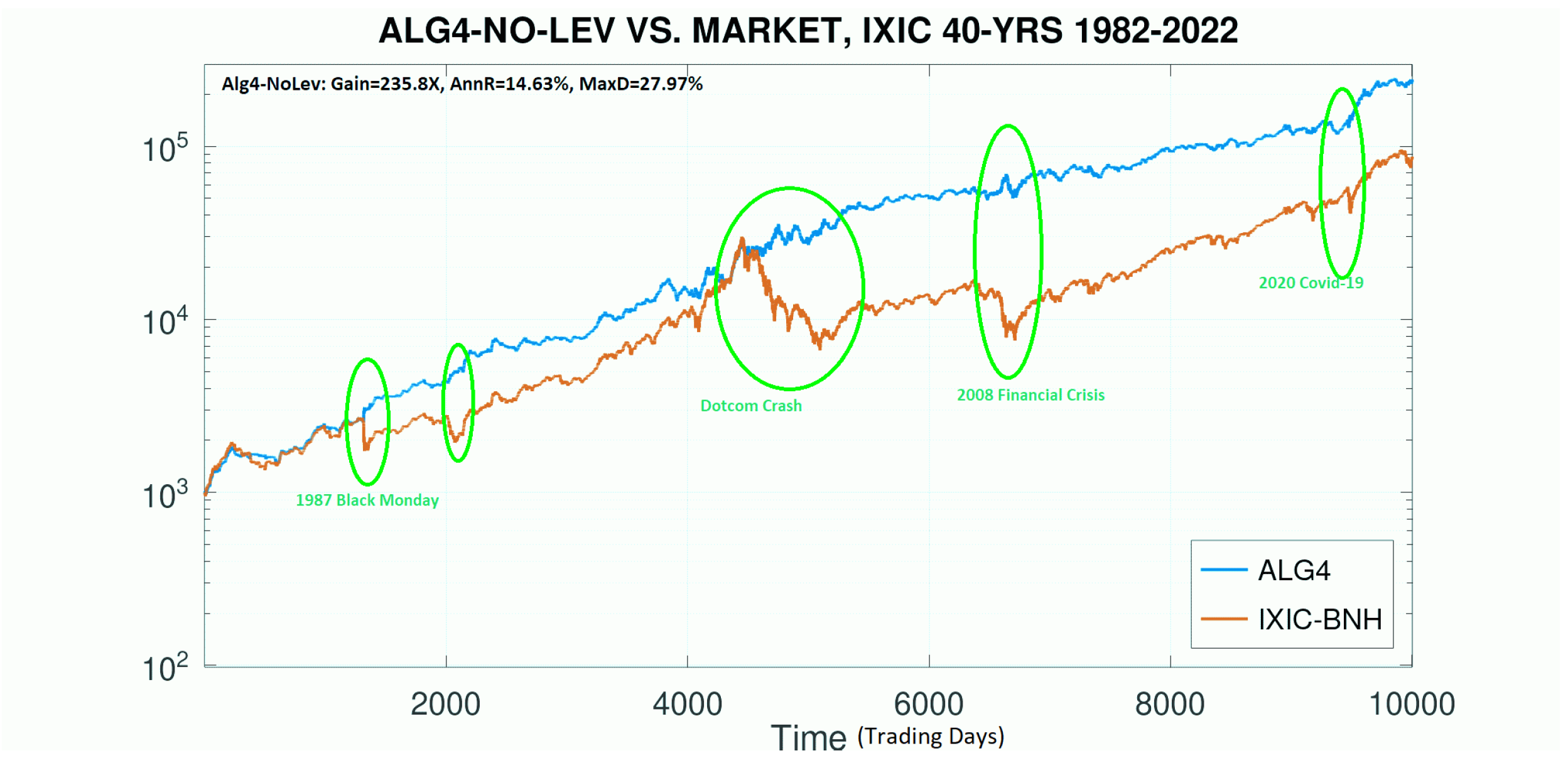
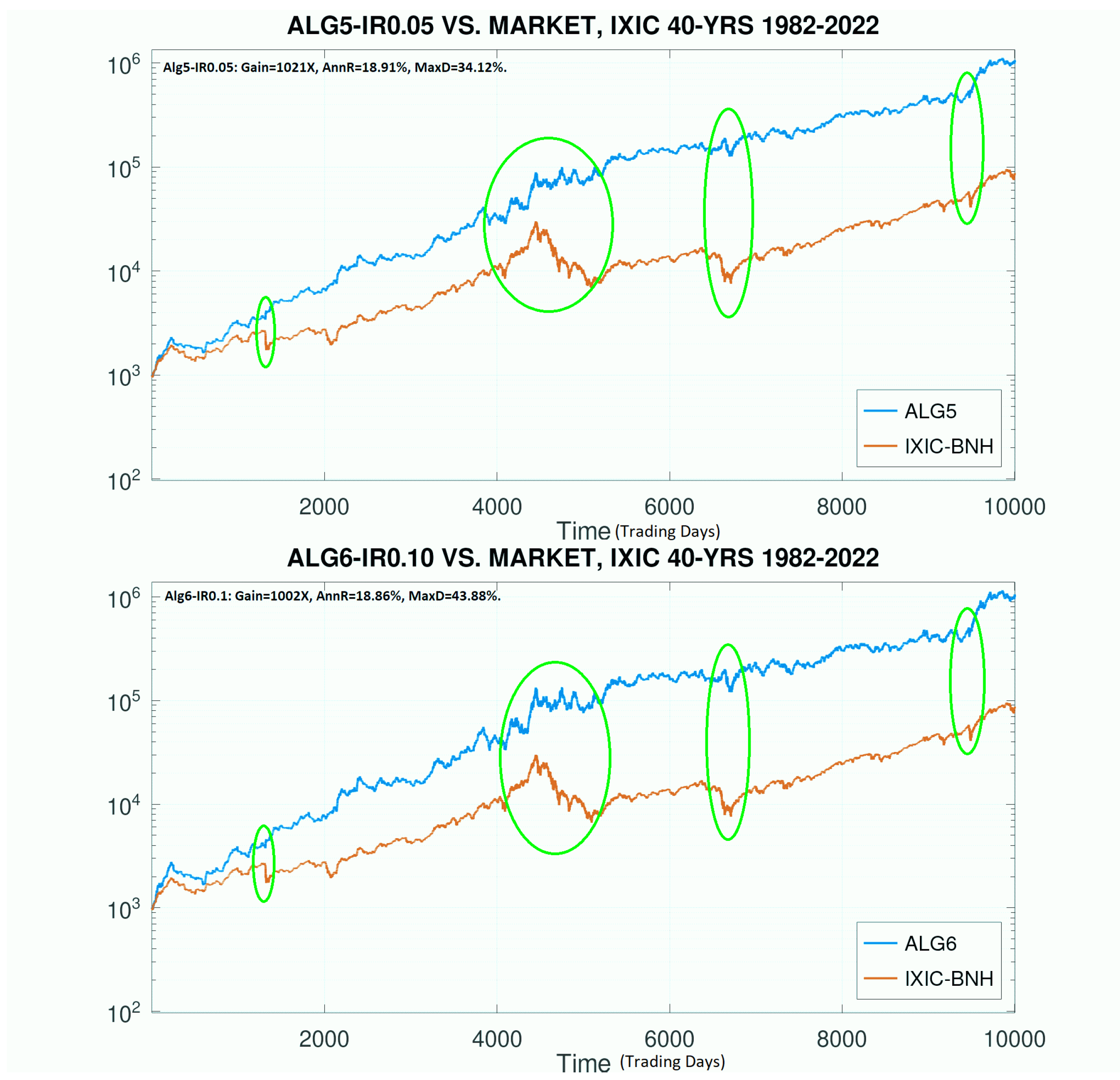
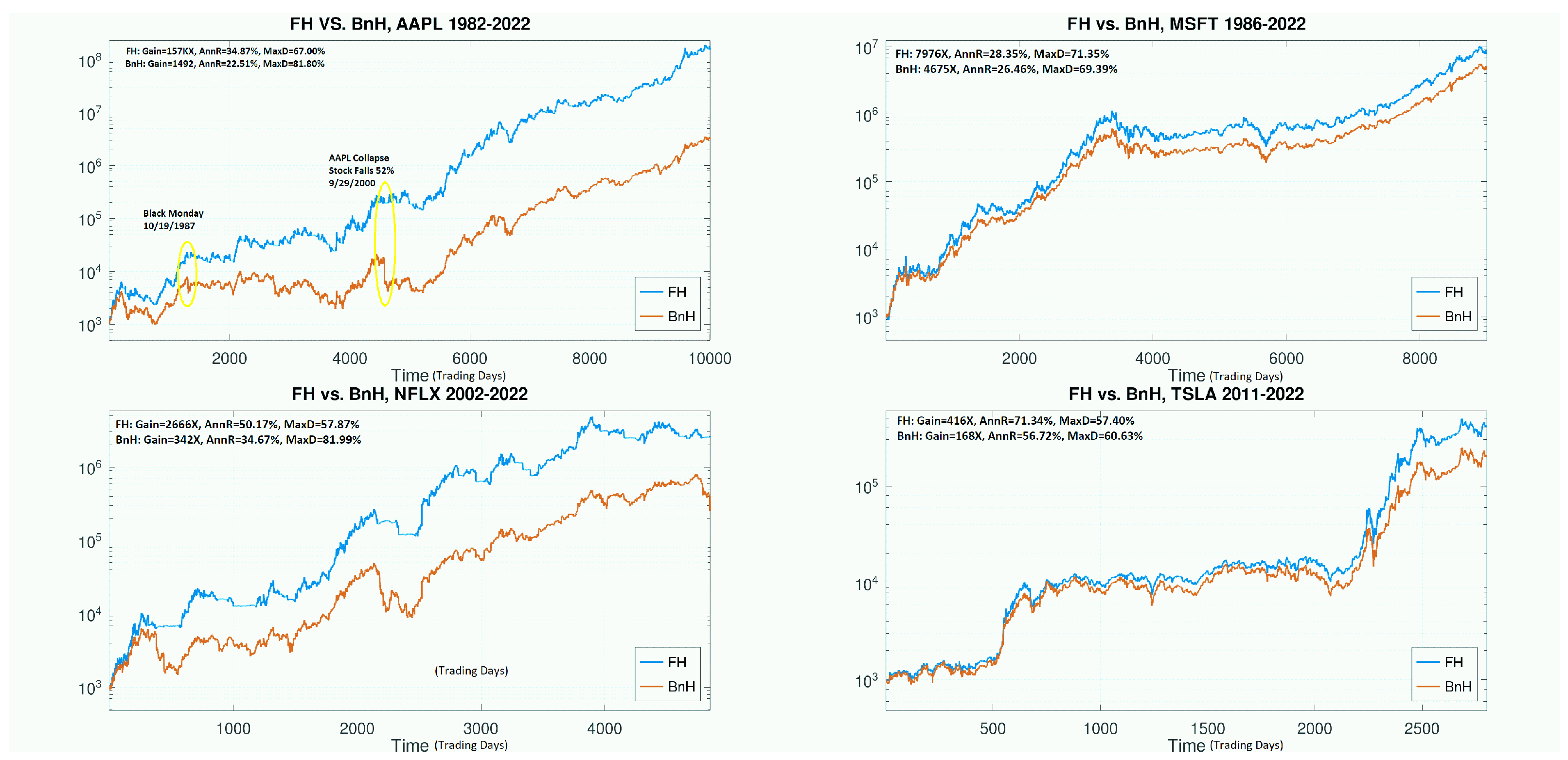
Publisher’s Note: MDPI stays neutral with regard to jurisdictional claims in published maps and institutional affiliations. |
© 2022 by the authors. Licensee MDPI, Basel, Switzerland. This article is an open access article distributed under the terms and conditions of the Creative Commons Attribution (CC BY) license (https://creativecommons.org/licenses/by/4.0/).