Article

On the Kavya–Manoharan–Burr X Model: Estimations under Ranked Set Sampling and Applications

by
Osama H. Mahmoud Hassan
1,*,
Ibrahim Elbatal
2,
Abdullah H. Al-Nefaie
1 and
Mohammed Elgarhy
3
1
Department of Quantitative Methods, School of Business, King Faisal University, Al-Ahsa 31982, Saudi Arabia
2
Department of Mathematics and Statistics, College of Science, Imam Mohammad Ibn Saud Islamic University (IMSIU), Riyadh 11564, Saudi Arabia
3
The Higher Institute of Commercial Sciences, Al Mahalla Al Kubra, Algarbia 31951, Egypt
*
Author to whom correspondence should be addressed.
J. Risk Financial Manag. 2023, 16(1), 19; https://doi.org/10.3390/jrfm16010019
Submission received: 10 November 2022 / Revised: 19 December 2022 / Accepted: 22 December 2022 / Published: 28 December 2022
(This article belongs to the Special Issue Stochastic Modeling and Statistical Analysis of Financial Data)

Abstract

:
A new two-parameter model is proposed using the Kavya–Manoharan (KM) transformation family and Burr X (BX) distribution. The new model is called the Kavya–Manoharan–Burr X (KMBX) model. The statistical properties are obtained, involving the quantile (QU) function, moment (MOs), incomplete MOs, conditional MOs, MO-generating function, and entropy. Based on simple random sampling (SiRS) and ranked set sampling (RaSS), the model parameters are estimated via the maximum likelihood (MLL) method. A simulation experiment is used to compare these estimators based on the bias (BI), mean square error (MSER), and efficiency. The estimates conducted using RaSS tend to be more efficient than the estimates based on SiRS. The importance and applicability of the KMBX model are demonstrated using three different data sets. Some of the useful actuarial risk measures, such as the value at risk and conditional value at risk, are discussed.

1. Introduction

Burr (1942) proposed twelve types of cumulative distribution functions (cdfs) for modeling lifespan data. The most common of these distributions are the BX and Burr type XII distributions. The fact that the BX distribution has a declining and growing hazard function is one of its key characteristics. The BX distribution has been used extensively in reliability research, agriculture, biology, and medicine. It may also be used to successfully represent strength data as well as to general lifespan data. Many researchers have examined several features of the BX distribution in recent years; for example, Surles and Padgett (2001) proposed a scaled BX distribution inference for reliability and stress–strength measurements. Aludaat et al. (2008) studied BX distribution parameter estimates for grouped data. Furthermore, Raqab and Kundu (2006) created a two-parameter BX distribution that is a closed variant of the generalized Rayleigh distribution and utilized it to simulate ball bearing data. Algarni et al. (2021) proposed the type I half-logistic Burr XG family and the bivariate Burr X generator of distributions, which were investigated by El-Morshedy et al. (2020). Bantan et al. (2021) discussed the truncated Burr X-G family of distributions. The cdf of the BX distribution is provided via the following equation:
G   B X ( x , α , β ) = [ 1 e ( α x ) 2 ] β , x , α , β > 0 ,
where α   and   β are positive scale and shape parameters, respectively. The associated density function (pdf) and hazard rate function (hrf) are respectively supplied with:
g   B X ( x , α , β ) = 2 β α 2 x e ( α x ) 2 [ 1 e ( α x ) 2 ] β 1 .
and
h   B X ( x , α , θ ) = 2 β α 2 x e ( α x ) 2 [ 1 e ( α x ) 2 ] β 1 [ 1 e ( α x ) 2 ] β
Depending on the shape parameter, the hrf of a BX distribution could be either a bathtub function or an increasing function. When β 1 2 , the hrf is a bathtub shape, and when β > 1 2 , the hrf is growing. Surles and Padgett (2005) demonstrated that the two-parameter BX distribution may be employed in modeling both strength and general lifespan data.
Statistical and applied academics are increasingly interested in constructing flexible lifespan models to improve the modeling of survival data. As a result, substantial work has been performed to generalize several well-known lifespan models, which have been successfully applied to difficulties in a wide range of scientific fields of study. Despite the fact that extra parameters give greater freedom, they also increase the complexity of the parameter estimation. Kumar et al. (2015) proposed a DUS (Dinesh–Umesh–Sanjay) transformation to produce a new parsimonious class of distributions to acquire new lifetime distributions. If G(x) is the baseline cdf, the DUS transformation yields the new cdf F(x), as shown below.
F ( x ) = e G ( x ) 1 e 1 .
The merit of using this transformation is that the resulting distribution retains the attribute of being parameter-sparse because no more parameters are added. Kavya and Manoharan (2020) proposed a generalized lifespan model based on the DUS transformation. The generalized DUS (GDUS) transformation’s cdf is provided via the following equation:
F ( x ; α , ζ ) = exp ( G α ( x ; ζ ) ) 1 e 1 , x > 0 ,
where α > 0 . The associated pdf is supplied with:
f ( x ; α , ζ ) = α g ( x ; ζ ) G α 1 ( x ; ζ ) exp ( G α ( x ; ζ ) ) e 1
where G ( x ; ζ ) is the baseline distribution and g ( x ; ζ )   is the parent pdf in the GDUS family. Because it is obviously a transformation rather than a generalization, it will yield a parsimonious distribution in terms of the computation and interpretation because it never contains any additional parameters other than those involved in the baseline distribution. Alotaibi et al. (2022b) proposed bivariate step stress accelerated life tests for the Kavya–Manoharan exponentiated Weibull model under a progressive censoring scheme. Alotaibi et al. (2022a) proposed the Kavya–Manoharan inverse-length biased exponential distribution under a progressive stress model based on progressive type-II censoring.
Recently, Kavya and Manoharan (2021) introduced a new transformation family, called the KM transformation family of distributions. The cdf is provided via:
F   K M ( x ) = e e 1 ( 1 e G ( x ) ) , x > 0 .
The associated pdf is supplied with:
f K M ( x ) = e e 1 g ( x ) e G ( x ) ,
and the hrf is:
h K M ( x ) = g ( x ) e 1 G ( x ) e 1 G ( x ) 1 .
Using a given baseline distribution, this family generates new lifespan models or distributions. They do not add any extra parameters to the model to keep it tuned to the current uncertainty, instead focusing on modeling the lifetime with a process that produces correct parsimonious findings. They chose the exponential and Weibull distributions as baseline distributions because they are widely used in reliability theory and survival analyses.
As our object in this article, we propose a new extension of the BX model based on the KM transformation family called the Kavya–Manoharan BX (KMBX) model. A battery of general features of the KMBX model is discussed. The KMBX model is developed using the maximum likelihood (ML) technique. It is applied to fit three data sets of biomedical and financial data. Using standard benchmarks, we reveal that it performs better than the selected competing models. The section of actuarial measures concerns useful risk measures, with a focus on the value at risk and conditional value at risk.
The remainder of the article is as follows. The second section presents the KMBX distribution as well as the density function expansion. Section 3 derives the QU function, median, MOs, incomplete MOs, MO-generating function, conditional MOs, mean residual lifetime, and Rényi entropy. Section 4 employs MLL estimates under SiRS and RaSS. In the same section, the simulation experiment is used to compare these estimators based on the BI, MSER, and efficiency. In Section 5, we highlight the significance of the existing model by studying real data applications to convey its efficiency and applicability. Some useful actuarial risk measures, such as the value at risk and conditional value at risk, are discussed in Section 6. Finally, the concluding remarks are mentioned in Section 7.

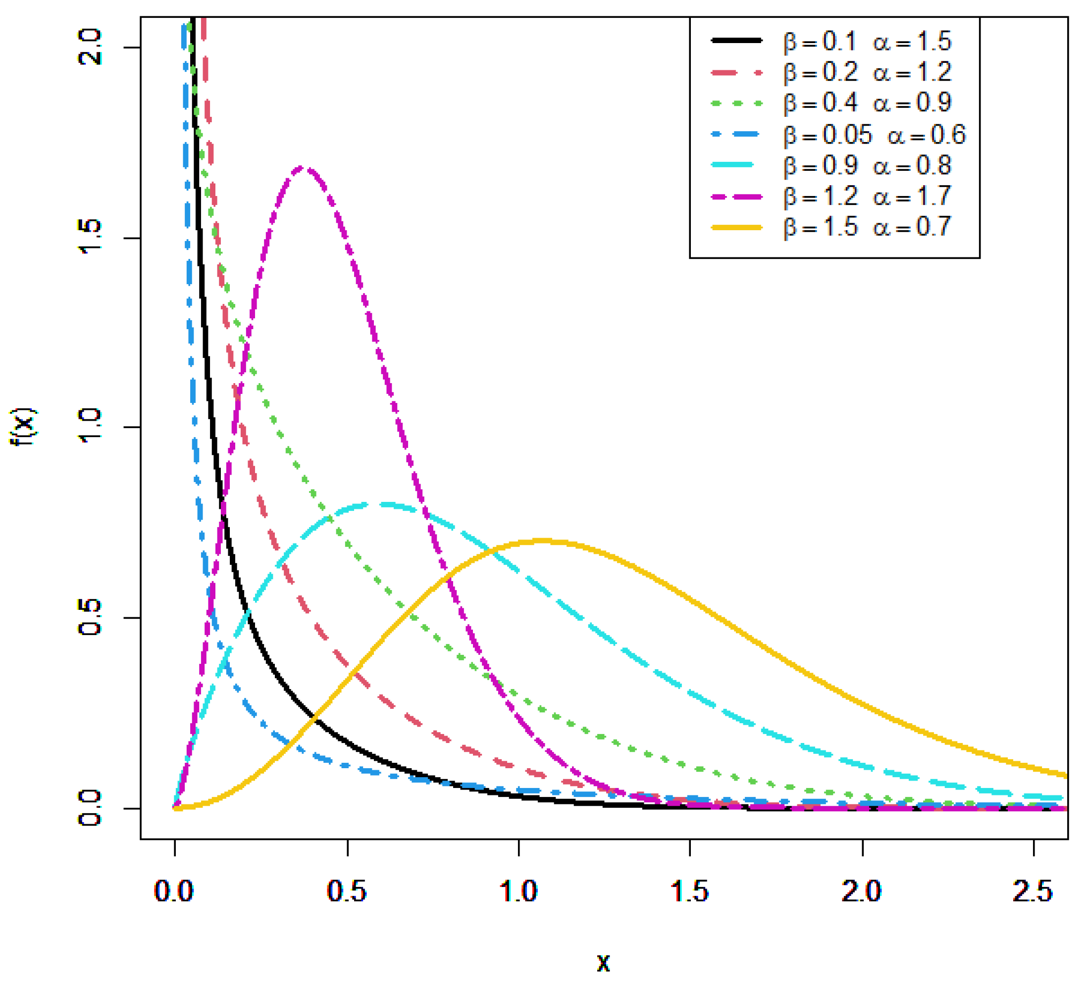
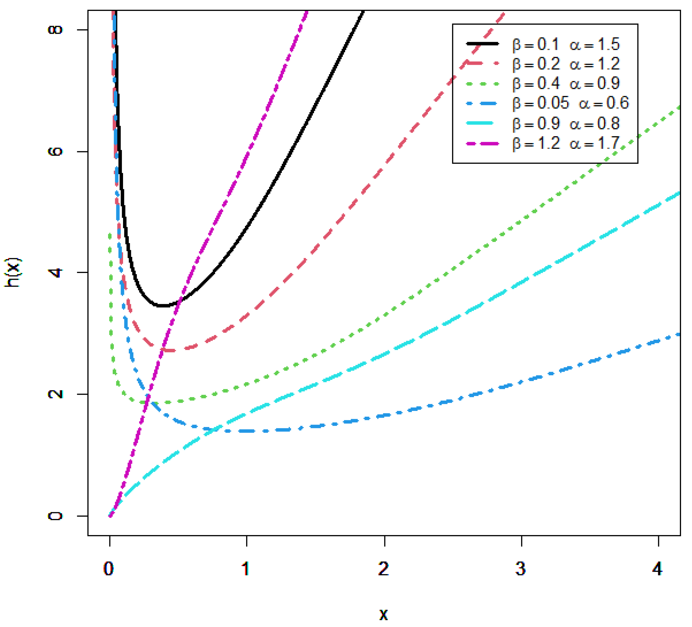
2. Kavya-Manoharan Burr X Distribution

We consider G ( x ) in Equation (7) to be the cdf of the Burr type X distribution given in Equation (1), so that the cdf of the KMBX distribution can be expressed as:
F   K M B X ( x ; α , β ) = e e 1 ( 1 e [ 1 e ( α x ) 2 ] β ) .
The corresponding pdf and hrf are provided via:
f   K M B X ( x ; α , β ) = 2 e β α 2 e 1 x e ( α x ) 2 [ 1 e ( α x ) 2 ] β 1 e [ 1 e ( α x ) 2 ] β ,
and:
h   K M B X ( x ; α , β ) = 2 e β α 2 e 1 x e ( α x ) 2 [ 1 e ( α x ) 2 ] β 1 e [ 1 e ( α x ) 2 ] β × 1 e e 1 ( 1 e [ 1 e ( α x ) 2 ] β ) .
Using the generalized binomial ( 1 z ) b 1 = j = 0 ( 1 ) j ( b 1 j ) z j , | z | < 1 and e x = i = 0 ( x ) i i ! , the expansion of the pdf in (11) may be expressed as below:
f   K M B X ( x ; α , β ) = i , j = 0 ϖ i , j x e ( j + 1 ) ( α x ) 2 ,
where:
ϖ i , j = 2 e β α 2 e 1 ( 1 ) i + j i ! ( θ ( i + 1 ) 1 j ) .
Hereafter, a random variable X that has the pdf from (11) is symbolized by X K M B X ( α , β ) .  Figure 1 and Figure 2 show the curves for the pdf and hazard rate function of the K M B X distribution.

3. Statistical Measures

In this section, we give some important statistical properties of the KMBX distribution, such as the QU function, median, MOs, incomplete MOs, MO-generating function, conditional MOs, mean residual lifetime, and Rényi entropy.

3.1. Quantile Function

The p th QU function of the KMBX distribution is supplied with:
x p = Q ( p ) = 1 α l o g { 1 [ l o g ( 1 p ( 1 e 1 ) ) ] 1 β } 1 2 ,
where p ( 0 , 1 ) . Additionally, when we put p = 0.5, we can get the median as below:
M e d i a n = 1 α l o g { 1 [ log ( 1 0.5 ( 1 e 1 ) ) ] 1 β } 1 2

3.2. Moments and Incomplete Moments

The statistical moments of different orders are important to define the uncertainty characteristics of the distributions. Using the expansion of (13), the r th MO of X is provided via:
μ r = x r f ( x ) d x = i , j = 0 ϖ i , j 0 x r + 1 e ( j + 1 ) ( α x ) 2 d x
setting y = ( j + 1 ) ( α x ) 2 , after using algebra, the r th MOs is provided with:
μ r = i , j = 0 ϖ i , j Γ ( r 2 + 1 ) 2 α r + 2 ( j + 1 ) r 2 + 1 .
Individually, the first four moments are obtained by setting r = 1, 2, 3, and 4 in (18). Additionally, the rth central moment ( μ r ) of X is given by:
μ r = E ( X μ 1 ) r = i = 0 r ( 1 ) i ( r i ) ( μ 1 ) i μ r i .
The skewness (SK) and kurtosis (Ku) are defined by:
S K = μ 3 μ 2 3 2 , K u = μ 4 μ 2 2 .
The s th incomplete MO of the KMB X distribution is expressed by:
η s ( t ) = E ( X s | X < t ) = 0 t x s f ( x ) d x
We can write the following equation from Equation (12):
η s ( t ) = i , j = 0 ϖ i , j γ ( s 2 + 1 , ( j + 1 ) ( α t ) β ) 2 α s + 2 ( j + 1 ) s 2 + 1 ,
where γ ( s , t ) = 0 t x s 1 e x d x is the lower incomplete gamma function.

3.3. Conditional Moments

For the KMBX distribution, it is easy to note that the conditional MOs E ( X s | X t ) can indeed be expressed as:
E ( X s | X t ) = 1 F ¯ ( t ) H s ( x ) ,
where:
H s ( x ) = t x s f ( x ) d x = i , j = 0 ϖ i , j Γ ( s 2 + 1 , ( j + 1 ) ( α t ) β ) 2 α s + 2 ( j + 1 ) s 2 + 1 ,
and Γ ( s , t ) = t x s 1 e x d x is the upper incomplete gamma function. An important application of the conditional MOs is the mean residual life (MRL) function. It is very important in terms of reliability and survival analyses, and it is used to model the burn-in and conservation of the component. For the KMBX distribution, the MRL function in terms of the first conditional MO is:
μ ( t ) = E ( ( X t ) | X t ) = 1 F ¯ ( t ) H 1 ( x ) t ,
where H 1 ( x ) is the first complete MOs following from (24) with s = 1 . Another application is the mean deviations about the mean μ and the median. They are used to measure the spread in a population from the center. The mean deviations about the mean and about the median are defined by δ μ = 2 μ   F   ( μ ) 2 μ + 2 H 1 ( μ ) and δ M = 2 H 1 ( M )     μ , respectively, where F ( μ ) is evaluated from (10), H 1 ( μ ) and H 1 ( M ) can be obtained from (24).

3.4. Moment-Generating Functions

The MO-generating function of the KMBX distribution can indeed be expressed as:
M X ( t ) = E ( e t X ) = 0 e t x f ( x ) d x = r = 0 t r r ! μ r        = i , j , r = 0 t r r ! ϖ i , j Γ ( r 2 + 1 ) 2 α r + 2 ( j + 1 ) r 2 + 1 .

3.5. Rényi Entropy

The Rényi entropy is provided via:
I   R ( δ ) = 1 1 ζ l o g [ 0 f   δ ( x ) d x ] ,   ρ > 0 , ρ 1 .
The Rényi entropy of X can indeed be expressed as:
I   R ( δ ) = 1 1 δ l o g { ( e β α 2 e 1 ) δ i , j = 0 2 δ 1 ( 1 ) i + j Γ ( δ + 1 2 ) i ! [ ( j + δ ) α 2 ] δ + 1 2 } .

4. Parameter Estimation

The MLL estimate of the KMBX model parameters is derived in this part using RaSS and RaSS. A simulation study is also carried out to compare the behavior of the estimators for both approaches.

4.1. MLL Approach under SiRS

We use the MLL estimates (MLLEs) approach to estimate the unknown parameters of the KMBX distribution in this part. We assume that x 1 , , x n is an n -th random sample (RS) from the KMBX distribution provided by (11). The KMBX distribution’s log-likelihood (log-LL) (L) function is provided via
L = n log ( 2 e e 1 ) + n log ( β ) + 2 n log ( α ) + i = 1 n log ( x i ) α 2 i = 1 n x i i = 1 n [ 1 e ( α x i ) 2 ] β + ( β 1 ) i = 1 n log [ 1 e ( α x i ) 2 ] .
Differentiating Equation (29) partially with regard to α and β to equate the results to 0, we get the following:
L α = 2 n α 2 α i = 1 n ( x i ) 2 α β i = 1 n x i 2 e ( α x i ) 2 [ 1 e ( α x i ) 2 ] β 1 + ( β 1 ) i = 1 n 2 α x i 2 e ( α x i ) 2 1 e ( α x i ) 2 ,
and:
L β = n β i = 1 n [ 1 e ( α x i ) 2 ] β log [ 1 e ( α x i ) 2 ] + i = 1 n log [ 1 e ( α x i ) 2 ] .
The MLLEs of parameters α and β symbolized by α ^ and β ^ , respectively, are investigated by solving the above non-linear system of equations simultaneously. As a result, we cannot get specific confidence ranges for the parameters. The large sample approximation must be used. It is known that the asymptotic distribution of the MLE φ ^ is ( φ ^ − φ)   N   ( 0 ,   I 1 ( φ ) ) , where   I 1 ( φ ) , and the inverse of the observed information matrix of the unknown parameters φ = ( α ,   β )   i s :
  I 1 ( φ ) = [   2 L φ 2   ] 1 ( α , β ) = ( α ^ ,   β ^ )
and whose elements are given in the Appendix A.

4.2. MLL Approach under RaSS

We assume X(i)ic, i = 1…m and c = 1…k is an RaSS from the KMBX model, which has sample size n = mk, where k is the number of cycles and m is the set size. We consider Yic = X(i)ic for simplicity, and for a given c, Yic is independent, with the pdf being equal to the pdf of the ith order statistics. The sample’s LL function y1c, y2c,…,ymc:
1 = c = 1 k i = 1 m m ! ( i 1 ) ! ( m i ) ! [ F ( y i c ) ] i 1 f ( y i c ) [ 1 F ( y i c ) ] m i = c = 1 k i = 1 m m ! ( i 1 ) ! ( m i ) ! [ e e 1 ( 1 e [ Q i c ] β ) ] i 1 2 e β α 2 e 1 y i c                     e [ ( α y i c ) 2 + [ Q i c ] β ] [ Q i c ] β 1 [ 1 e e 1 ( 1 e [ Q i c ] β ) ] m i ,
where Q i c = 1 e ( α y i c ) 2 . The log-LL function of the KMBX distribution under RaSS is provided via:
ln 1 = ln c + m k ln β + 2 m k ln α + c = 1 k i = 1 m l n ( y i c ) c = 1 k i = 1 m [ ( α y i c ) 2 + [ Q i c ] β ] + ( β 1 ) c = 1 k i = 1 m l n ( Q i c )         + c = 1 k i = 1 m ( i 1 ) l n [ 1 e [ Q i c ] β ]    + c = 1 k i = 1 m ( m i ) l n [ 1 e e 1 ( 1 e [ Q i c ] β ) ] .
Differentiating Equation (34) partially with regard to α and β and equating the results to 0, we can solve the non-linear system of equations simultaneously. Then, we can get the MLLEs of parameters α and β symbolized by α ^ and β ^ , respectively, using the Mathematica (10) software program.

4.3. Numerical Outcomes

This subsection describes the numerical investigation used to derive the MLLEs of the population parameters for the KMBX distribution using RaSS and SiRS. A comparative study is carried out by comparing estimates in terms of the MSERs, biases, and relative efficiency (REEF). The following algorithm describes the simulation techniques.
First procedure: The RS measuring n = 50, 150, 250, 500, and 1000 with m = n , k = n are generated from KMBX model, where n 2 = m × k . After this, we rank one observation from each cycle.
Second procedure: The numerical values of the parameter are chosen.
Third procedure: The MLLEs are calculated under SiRS and RaSS for the given set of parameters and each n.
Fourth procedure: We repeat the above procedures from the first to third N times representing various samples, where N = 1000. After this, the BIs, MSERs, and REEF = MSER (RaSS)/MSER (SiRS) of the estimates are investigated.
Fifth procedure: Table 1, Table 2, Table 3, Table 4, Table 5 and Table 6 provide the numerical results.
Considering Table 1, Table 2, Table 3, Table 4, Table 5 and Table 6, the relevant points should be noted:
  • The BIs and MSERs for the estimations depending on SiRS are greater than the comparable values depending on RaSS;
  • In most scenarios, the BIs and MSER decrease as the n rises for both sampling strategies;
  • In most cases, the efficiency of the estimates rises as the sample numbers grow;
  • The MLLEs depending on RaSS have lower MSER values than the corresponding values depending on SiRS.

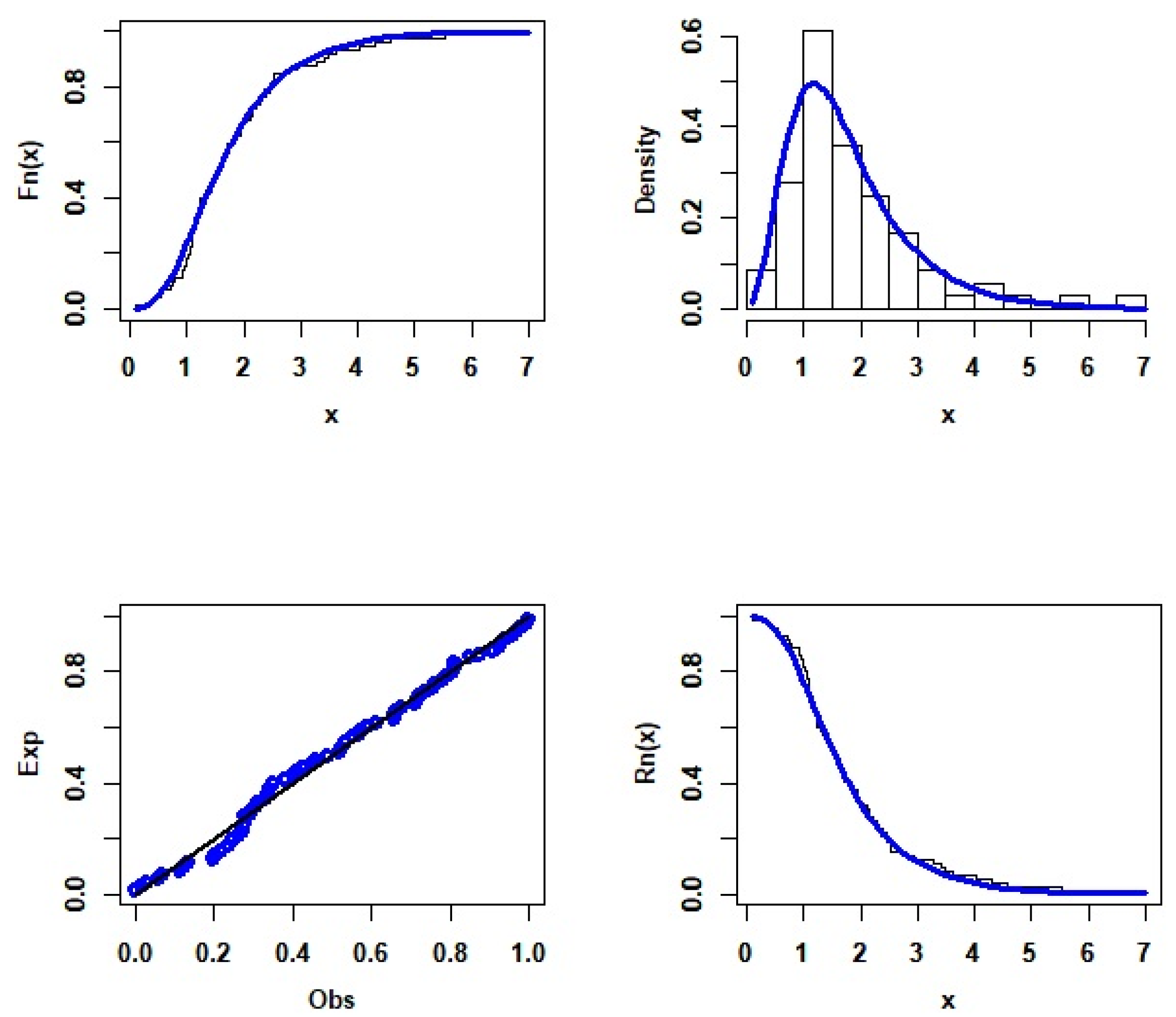
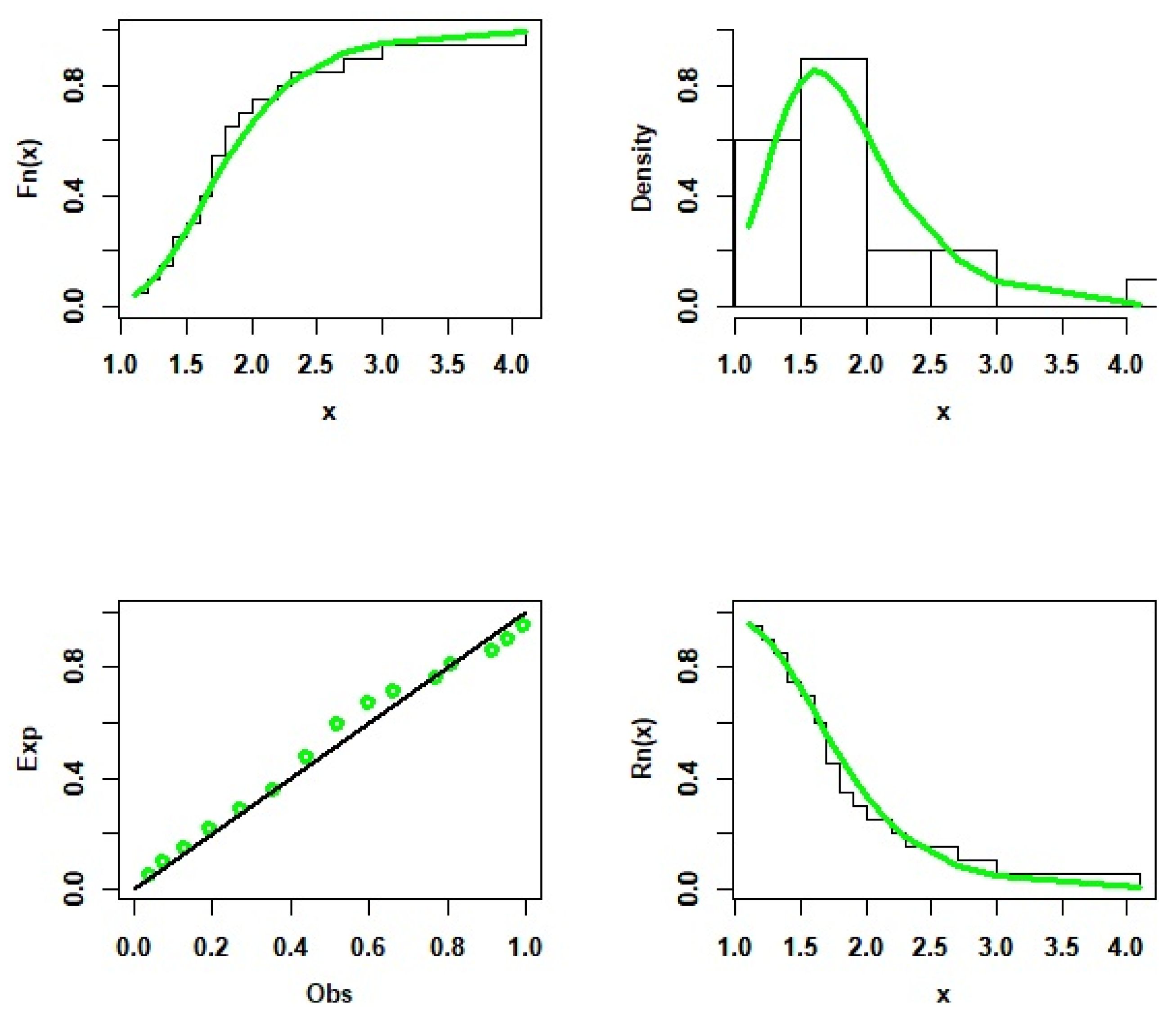
5. Application to Real Data Sets

Here, in this section, we demonstrate the usefulness of the KMBX model by using three data sets. Numerous researchers have utilized these data to demonstrate the applicability of competing models. We additionally offer a formative assessment of the models’ goodness of fit and draw comparisons with other continuous models that have one, two, three, four, five, and six parameters. The goodness of fit measures comprise the Akaike information criterion (INC) ( 1 ), consistent Akaike INC ( 2 ), Bayesian INC ( 3 ), and Hannan–Quinn INC ( 4 ), which are calculated in order to compare the fitted models. The smaller the values of these statistics, generally the superior the match to both data sets.
  • The First Data Set: Survival Times Data
The first data set was studied by Bjerkedal in 1960, representing the survival times (in days) of 72 guinea pigs infected with virulent tubercle bacilli. For these data, shall compared the ts of the KMBX distribution with the exponential (E), Marshall–Olkin E (MOLE), Burr X-E (BXE), Kumaraswamy E (KE), beta E (BE), Kumaraswamy MOLE (KMOLE), generalized MOLE (GMOLE), MOL Kumaraswamy E (MOLKE), and moment E (ME) models (see Refaie 2018).
  • The Second Data Set: Relief Times Data
This set of data contained only the relief times of 20 patients who received an analgesic (Gross and Clark 1975). For these data, we compared the KMBX distribution with the MOLE, BXE, KE, BE, KMOLE, GMOLE, Ailamujia (A) (Lv et al. 2002), inverse A (IA) (Aijaz et al. 2020), E, McDonald (MC) log-logistic (MCLOL) (Tahir et al. 2014), MCWeibull (MCW) (Cordeiro et al. 2014), beta (B) generalized inverse Weibull geometric distribution (BGIWG) (Elbatal et al. 2017), B transmuted (TR) Weibull (BTRW) (Afify et al. 2017), new modified Weibull (NMW) (Almalki and Yuan 2013), TR complementary Weibull-geometric (TRCWG) (Afify et al. 2014), B Weibull (BW) (Lee et al. 2007), exponentiated TR generalized Rayleigh (ETRGR) (Ahmed et al. 2015), Weibull–Lomax (WL) (Tahir et al. 2015), TR Weibull–Lomax (TRWL) (Afify et al. 2015), Burr XII, Kumaraswamy–Weibull–exponential (KWE) (ZeinEldina and Elgarhyc 2018), Weibull (W), gamma-Chen (CH) (GCH) (Alzaatreh et al. 2014), beta-CH (BCH) (Eugene et al. 2002), Marshall–Olkin CH (MOCH) (Jose 2011), TR Chen (TRCH) (Khan et al. 2013), TR exponentiated CH (TRECH) (Khan et al. 2016), and CH distributions.
  • The Third Data Set: Financial Data
The third data set was studied by Mead in 2014, containing actual monthly tax revenues from Egypt from January 2006 to November 2010. For these data, we compared the KMBX distribution with the BX, E, MOLE, exponentiated Weibull (EW), odd Weibull exponential (OWE), and Weibull (W) models. The profile log-likelihood plots are shown in Figure 3, Figure 4 and Figure 5.
The estimated parameters along with their Ser values and the statistics for the fitted models are provided in Table 7, Table 8, Table 9, Table 10, Table 11 and Table 12. We note from Table 8, Table 10, and Table 12 that the KMBX gives the smallest values of 1 ,   2 , 3 , and   4 as compared to the other competitive models. Therefore, the KMBX distribution provides the best t for the three data sets. More information can be found in Figure 6, Figure 7 and Figure 8.
Based on the numerical results acquired in Table 8, Table 10, and Table 12, we found that our model had the lowest values for 1 ,   2 , 3 , and   4 . Figure 6, Figure 7 and Figure 8 all supported these numerical results, showing that the KMBX model is the best model for fitting the three data sets.

6. Actuarial Measures

In this part, we compute certain key risk measures for the recommended distribution, such as the value at risk and conditional value at risk, which are vital for strategy optimization despite uncertainty.

6.1. Value at Risk

If X ∼ KMBX denotes a random variable with the cdf from (10), then its value at risk is:
R V ν = 1 α l o g { 1 [ log ( 1 ν ( 1 e 1 ) ) ] 1 β } 1 2 .

6.2. Conditional Value at Risk

Instead of using the value at risk, Artzner (1997, 1999) suggested using the conditional value at risk. The conditional value at risk is typically used to calculate the mean loss in cases where the value at risk exceeds the nominal values by a significant amount. The next expression serves as its definition:
C R V ν = 1 ν 0 ν R V ν d ν ,                      0 < ν < 1 .
The conditional value at risk of the KMBX is provided via:
C R V ν = 1 ν 0 ν = 1 α l o g { 1 [ log ( 1 ν ( 1 e 1 ) ) ] 1 β } 1 2 d ν ,               0 < ν < 1 .

7. Conclusions

In this research, we investigated the Kavya–Manoharan–Burr X (KMBX) model, which has two parameters. Its statistical and mathematical features (QU function, median, MOs, incomplete MOs, MO-generating function, conditional MOs, mean residual lifetime, and Rényi entropy) were derived. Based on SiRS and RaSS, the model parameters were estimated using the MLL method. A simulation experiment was used to compare these estimators based on the BI, MSER, and efficiency. The relevance and flexibility of the KMBX model were demonstrated using three real data sets. The new suggested model was superior to some well-known models in the modeling of the proposed data. We compared our model with twenty-nine other models, and our model gave the best fit for the data. Some useful actuarial risk measures, such as the value at risk and conditional value at risk, were also discussed.

Author Contributions

Conceptualization, O.H.M.H. and I.E.; methodology, A.H.A.-N.; software, M.E.; validation, O.H.M.H. and I.E.; formal analysis A.H.A.-N.; investigation, A.H.A.-N.; resources, A.H.A.-N.; data curation, M.E.; writing—original draft preparation, M.E.; writing—review and editing, O.H.M.H. and I.E.; visualization, O.H.M.H.; supervision, O.H.M.H. and I.E.; project administration, A.H.A.-N.; funding acquisition, O.H.M.H. All authors have read and agreed to the published version of the manuscript.

Funding

The authors appreciate The Deanship of Scientific Research, Vice Presidency for Graduate Studies and Scientific Research, King Faisal University, Saudi Arabia, grant no. 846.

Data Availability Statement

The data used to support the findings of this study are available from the corresponding author upon request.

Acknowledgments

The authors appreciate The Deanship of Scientific Research, Vice Presidency for Graduate Studies and Scientific Research, King Faisal University, Saudi Arabia, grant no. 846.

Conflicts of Interest

The authors declare no conflict of interest.

Appendix A

The second-order partial derivatives of the log-likelihood function of the KMBX with respect to α, β are given by:
2 L α 2 = 2 n α 2 2 i = 1 n x i 2 β i = 1 n x i 2 e ( α x i ) 2 [ 1 e ( α x i ) 2 ] β 1 + 4 α 2 β i = 1 n x i 4 e ( α x i ) 2 [ 1 e ( α x i ) 2 ] β 1 4 α 2 β ( β 1 ) i = 1 n x i 4 e 2 ( α x i ) 2 [ 1 e ( α x i ) 2 ] β 1 + ( β 1 ) i = 1 n 2 x i 2 ( e ( α x i ) 2 1 ) 4 α 2 x i 4 e ( α x i ) 2 ( e ( α x i ) 2 1 ) 2 ,
2 L α β = 2 α β i = 1 n x i 2 e ( α x i ) 2 [ 1 e ( α x i ) 2 ] β 1 log [ 1 e ( α x i ) 2 ] + i = 1 n 2 α x i 2 [ 1 e ( α x i ) 2 ] β e ( α x i ) 2 1 + i = 1 n 2 α x i 2 e ( α x i ) 2 1 .
and:
2 L β 2 = n β 2 i = 1 n [ 1 e ( α x i ) 2 ] β ( log [ 1 e ( α x i ) 2 ] ) 2 .

References

  1. Afify, Ahmed Z., Zohdy M. Nofal, and Nadeem Shafique Butt. 2014. Transmuted complementary Weibull geometric distribution. Pakistan Journal of Statistics and Operations Research 10: 435–54. [Google Scholar] [CrossRef] [Green Version]
  2. Afify, Ahmed Z., Zohdy M. Nofal, Haitham M. Yousof, Yehia M. El Gebaly, and Nadeem Shafique Butt. 2015. Transmuted Weibull Lomax distribution. Pakistan Journal of Statistics and Operations Research 11: 135–52. [Google Scholar] [CrossRef] [Green Version]
  3. Afify, Ahmed, Haitham Yousof, and Saralees Nadarajah. 2017. The beta transmuted-H family for lifetime data. Statistics and Its Interface 10: 505–20. [Google Scholar] [CrossRef] [Green Version]
  4. Ahmed, Z., Zohdy M. Nofal, and N. Ebraheim Abd El Hadi. 2015. Exponentiated transmuted generalized Rayleigh distribution: A new four parameter Rayleigh distribution. Pakistan Journal of Statistics and Operations Research 11: 115–34. [Google Scholar]
  5. Aijaz, Ahmad, Afaq Ahmad, and Rajnee Tripathi. 2020. Inverse Analogue of Ailamujia Distribution with Statistical Properties and Applications. Asian Research Journal of Mathematics 16: 36–46. [Google Scholar] [CrossRef]
  6. Algarni, Ali, Abdullah M. Almarashi, I. Elbatal, Amal S. Hassan, Ehab M. Almetwally, Abdulkader M. Daghistani, and Mohammed Elgarhy. 2021. Type I half logistic Burr XG family: Properties, Bayesian, and non-Bayesian estimation under censored samples and applications to COVID-19 data. Mathematical Problems in Engineering 2021: 5461130. [Google Scholar] [CrossRef]
  7. Almalki, Saad J., and Jingsong Yuan. 2013. A new modified Weibull distribution. Reliability Engineering and System Safety 111: 164–70. [Google Scholar] [CrossRef]
  8. Alotaibi, Naif, Atef F. Hashem, Ibrahim Elbatal, Salem A. Alyami, A. S. Al-Moisheer, and Mohammed Elgarhy. 2022a. Inference for a Kavya–Manoharan Inverse Length Biased Exponential Distribution under Progressive-Stress Model Based on Progressive Type-II Censoring. Entropy 24: 1033. [Google Scholar] [CrossRef]
  9. Alotaibi, Naif, Ibrahim Elbatal, Ehab M. Almetwally, Salem A. Alyami, A. S. Al-Moisheer, and Mohammed Elgarhy. 2022b. Bivariate Step-Stress Accelerated Life Tests for the Kavya–Manoharan Exponentiated Weibull Model under Progressive Censoring with Applications. Symmetry 14: 1791. [Google Scholar] [CrossRef]
  10. Aludaat, K. M., Moh’D Taleb Alodat, and Tareq Alodat. 2008. Parameter estimation of Burr type X distribution for grouped data. Applied Mathematical Sciences 2: 415–23. [Google Scholar]
  11. Alzaatreh, Ayman, Felix Famoye, and Carl Lee. 2014. The gamma-normal distribution: Properties and applications. Computational Statistics and Data Analysis 69: 67–80. [Google Scholar] [CrossRef]
  12. Artzner, Philippe. 1997. Thinking Coherently. Risk 10: 68–71. [Google Scholar]
  13. Artzner, Philippe. 1999. Application of coherent risk measures to capital requirements in insurance. North American Actuarial Journal 3: 11–25. [Google Scholar] [CrossRef]
  14. Bantan, Rashad A. R., Christophe Chesneau, Farrukh Jamal, Ibrahim Elbatal, and Mohammed Elgarhy. 2021. The Truncated Burr X-G Family of Distributions: Properties and Applications to Actuarial and Financial Data. Entropy 23: 1088. [Google Scholar] [CrossRef] [PubMed]
  15. Burr, Irving W. 1942. Cumulative frequency functions. The Annals of Mathematical Statistics 13: 215–32. [Google Scholar] [CrossRef]
  16. Cordeiro, Gauss M., Elizabeth M. Hashimoto, and Edwin M. M. Ortega. 2014. The McDonald Weibull model. Statistics 48: 256–78. [Google Scholar] [CrossRef]
  17. Elbatal, I., Yehia M. El Gebaly, and Essam A. Amin. 2017. The beta generalized inverse Weibull geometric distribution and its applications. Pakistan Journal of Statistics and Operation Research 13: 75–90. [Google Scholar] [CrossRef] [Green Version]
  18. El-Morshedy, M., Ziyad Ali Alhussain, Doaa Atta, Ehab M. Almetwally, and M. S. Eliwa. 2020. Bivariate Burr X generator of distributions: Properties and estimation methods with applications to complete and type-II censored samples. Mathematics 8: 264. [Google Scholar] [CrossRef] [Green Version]
  19. Eugene, Nicholas, Carl Lee, and Felix Famoye. 2002. Beta-normal distribution and its applications. Communications in Statistics-Theory and Methods 31: 497–512. [Google Scholar] [CrossRef]
  20. Gross, Alan J., and Virginia Clark. 1975. Survival Distributions: Reliability Applications in the Biomedical Sciences. New York: John Wiley and Sons. [Google Scholar]
  21. Jose, K. K. 2011. Marshall-Olkin family of distributions and their applications in reliability theory, time series modeling and stress-strength analysis. Paper presented at ISI 58th World Statistics Congress International Statistical Institute, Dublin, Ireland, August 21–26; pp. 3918–23. [Google Scholar]
  22. Kavya, P., and M. Manoharan. 2020. On a Generalized lifetime model using DUS transformation. In Applied Probability and Stochastic Processes. Infosys Science Foundation Series. Edited by V. Joshua, S. Varadhan and V. Vishnevsky. Singapore: Springer, pp. 281–91. [Google Scholar]
  23. Kavya, P., and M. Manoharan. 2021. Some parsimonious models for lifetimes and applications. Journal of Statistical Computation and Simulation 91: 3693–708. [Google Scholar] [CrossRef]
  24. Khan, Muhammad Shuaib, Robert King, and Irene Hudson. 2013. A new three parameter transmuted Chen lifetime distribution with application. Journal of Applied Statistical Science 21: 239–59. [Google Scholar]
  25. Khan, Muhammad Shuaib, Robert King, and Irene Lena Hudson. 2016. Transmuted exponentiated Chen distribution with application to survival data. ANZIAM Journal 57: 268–90. [Google Scholar] [CrossRef] [Green Version]
  26. Kumar, Dinesh, Umesh Singh, and Sanjay Kumar Singh. 2015. A method of proposing new distribution and its application to bladder cancer patients data. Journal of Statistics Applications and Probability Letters 2: 235–45. [Google Scholar]
  27. Lee, Carl, Felix Famoye, and Olugbenga Olumolade. 2007. Beta-Weibull distribution: Some properties and applications to censored data. Journal of Modern Applied Statistical Methods 6: 173–86. [Google Scholar] [CrossRef]
  28. Lv, H. Q., L. H. Gao, and C. L. Chen. 2002. Ailamujia distribution and its application in support ability data analysis. Journal of Academy of Armored Force Engineering 16: 48–52. [Google Scholar]
  29. Raqab, Mohammad Z., and Debasis Kundu. 2006. Burr type X distribution: Revisited. Journal of Probability and Statistical Sciences 4: 179–93. [Google Scholar]
  30. Refaie, Mohamed K. A. 2018. Burr X exponentiated exponential distribution. Journal of Statistics and Applications 1: 71–88. [Google Scholar]
  31. Surles, J. G., and W. J. Padgett. 2001. Inference for reliability and stress-strength for a scaled Burr type X distribution. Lifetime Data Analysis 7: 187–200. [Google Scholar] [CrossRef]
  32. Surles, J. G., and W. J. Padgett. 2005. Some properties of a scaled Burr type X distribution. Journal of statistical planning and inference 128: 271–80. [Google Scholar] [CrossRef]
  33. Tahir, Muhammad H., Gauss M. Cordeiro, M. Mansoor, and Muhammad Zubair. 2015. The Weibull-Lomax distribution: Properties and applications. Hacettepe Journal of Mathematics and Statistics 44: 455–74. [Google Scholar] [CrossRef]
  34. Tahir, Muhammad Hussain, Muhammad Mansoor, Muhammad Zubair, and Gholamhossein Hamedani. 2014. McDonald log logistic distribution with an application to breast cancer data. Journal of Statistical Theory and Applications 13: 65–82. [Google Scholar] [CrossRef] [Green Version]
  35. ZeinEldina, Ramadan A., and M. Elgarhyc. 2018. A new generalization of Weibull-exponential distribution with application. Journal of Nonlinear Science and Applications 11: 1099–112. [Google Scholar] [CrossRef]
Figure 1. The pdf plots of the KMBX model.
Jrfm 16 00019 g001
Figure 2. The hrf plots of the KMBX model.
Jrfm 16 00019 g002
Figure 3. The profile log-likelihood plot for the first data set.
Jrfm 16 00019 g003
Figure 4. The profile log-likelihood plot for the second data set.
Jrfm 16 00019 g004
Figure 5. The profile log-likelihood plot for the third data set.
Jrfm 16 00019 g005
Figure 6. The fitted cdf, pdf, and pp plots and the estimated plot for the first data set.
Jrfm 16 00019 g006
Figure 7. The fitted cdf, pdf, and pp plots and the estimated plot for the second data.
Jrfm 16 00019 g007
Figure 8. The fitted cdf, pdf, and pp plots and the estimated plot for the third data.
Jrfm 16 00019 g008
Table 1. The MLLEs, BIs, MSER, and REEF of the KMBX model under SiRS and RaSS at α = 0.9, β = 0.5.
nSiRSRaSSREEF
MLLEBIMSERMLLEBIMSER
500.964940.064940.023020.914080.014080.003640.15794
0.566630.066630.029050.504240.004240.002720.09348
1500.925640.025640.013940.89715−0.002860.000960.06905
0.49715−0.002850.008010.49692−0.003080.000800.09998
2500.915920.015920.004390.900130.000130.000190.04265
0.505870.005870.002860.501620.001620.000150.05289
5000.906980.006980.002270.89978−0.000220.000170.07597
0.510650.010650.001790.49973−0.000270.000140.07568
10000.89338−0.006620.000870.89998−0.000020.000030.03759
0.49586−0.004150.000520.500360.000360.000030.05376
Table 2. The MLLEs, BIs, MSER, and REEF of the KMBX model under SiRS and RaSS at α = 0.7, β = 1.2.
nSiRSRaSSREEF
MLLEBIMSERMLLEBIMSER
500.711990.011980.016410.69496−0.005040.002040.12425
1.233710.033710.077651.18874−0.011260.014650.18867
1500.701280.001280.004120.703410.003410.000520.12526
1.218430.018430.053811.217440.017440.004860.09033
2500.710350.010350.002810.69710−0.002900.000140.05060
1.213970.013970.014231.19018−0.009820.001570.11022
5000.701680.001680.001320.69931−0.000700.000050.04155
1.223490.023490.010041.19994−0.000060.000760.07581
10000.700550.000550.000370.69965−0.000360.000030.08976
1.218960.018960.005041.201060.001060.000290.05743
Table 3. The MLLEs, BIs, MSER, and REEF of the KMBX model under SiRS and RaSS at α = 1.2, β = 0.8.
nSiRSRaSSREEF
MLLEBIMSERMLLEBIMSER
501.232910.032910.049861.222580.022580.007770.15578
0.821140.021130.035980.820700.020700.006010.16693
1501.203900.003900.027851.18876−0.011240.002550.09166
0.79966−0.000340.013550.78934−0.010660.001610.11864
2501.234910.034910.007371.19494−0.005060.000470.06430
0.842200.042200.009670.79098−0.009020.000640.06587
5001.200880.000880.006001.19423−0.005770.000340.05708
0.79162−0.008380.006180.79611−0.003890.000290.04713
10001.19978−0.000220.002281.19724−0.002760.000100.04262
0.812490.012490.001630.79893−0.001070.000090.05454
Table 4. The MLLEs, BIs, MSER, and REEF of the KMBX model under SiRS and RaSS at α = 0.5, β = 0.5.
nSiRSRaSSREEF
MLLEBIMSERMLLEBIMSER
500.502850.002850.005120.503860.003860.000730.14321
0.49913−0.000870.017640.518840.018840.005700.32300
1500.505290.005290.002300.506980.006980.000310.13363
0.521270.021270.016390.518850.018850.001810.11041
2500.510100.010100.001720.49867−0.001330.000060.03632
0.522920.022920.007400.49353−0.006470.000370.04959
5000.505590.005590.000560.500380.000370.000040.06248
0.49469−0.005310.002750.501020.001020.000180.06560
10000.500330.000330.000180.500460.000460.000010.06492
0.501080.001080.000640.501630.001630.000080.12523
Table 5. The MLLEs, BIs, MSER, and REEF of the KMBX model under SiRS and RaSS at α = 1.5, β = 1.2.
nSiRSRaSSREEF
MLLEBIMSERMLLEBIMSER
501.594460.094460.117201.533480.033480.016380.13979
1.358380.158380.153401.221610.021610.011850.07722
1501.586300.086300.036461.47738−0.022620.003380.09269
1.265620.065620.034141.17926−0.020740.003040.08898
2501.528350.028360.016871.509140.009140.000860.05073
1.227960.027960.016951.211890.011890.000830.04872
5001.49492−0.005080.005491.502260.002260.000580.10633
1.18883−0.011170.006621.201710.001710.000450.06753
10001.49477−0.005230.003231.504600.004600.000170.05218
1.200180.000180.002601.203800.003800.000150.05880
Table 6. The MLLEs, BIs, MSER, and REEF of the KMBX model under SiRS and RaSS at α = 0.8, β = 0.8.
nSiRSRaSSREEF
MLLEBIMSERMLLEBIMSER
500.888570.088570.021690.804730.004720.002240.10323
0.855320.055320.039410.807650.007650.004430.11247
1500.803400.003400.009420.804610.004610.000670.07145
0.845450.045450.031420.807450.007450.002180.06927
2500.828810.028810.004740.801710.001710.000150.03126
0.822890.022890.014060.800720.000720.000640.04558
5000.79461−0.005390.002980.800890.000890.000080.02542
0.79290−0.007100.006430.802030.002030.000290.04512
10000.79628−0.003720.000550.800680.000680.000050.09571
0.79694−0.003060.001530.79923−0.000770.000200.13225
Table 7. Numerical values of MLLEs and (SErs) for the first data set.
ModelsMLLEs and SErs
KMBX (α, β)0.443
(0.038)
1.081 (0.153)
KMOLE (α, μ, τ, β)0.373
(0.136)
3.478 (0.862)3.306 (0.781)0.299 (1.113)
BXE (θ, β)0.475
(0.06)
0.206 (0.012)
GMOLE (λ, α, β)0.179
(0.07)
47.640 (44.90)4.47 (1.33)
BE (μ, τ, β)0.807
(0.70)
3.461 (1.003)1.3311 (0.8551)
KE (μ, τ, β)3.304
(1.1061)
1.1 (0.76)1.037 (0.614)
MOLKE (α, μ, τ, β)0.01
(0.002)
2.7162 (1.3158)1.99 (0.784)0.099 (0.05)
MOLE (α, β)8.778
(3.555)
1.3788 (0.1929)
ME (β)0.925
(0.077)
E (β)0.540
(0.06)
Table 8. Numerical values of 1 , 2 , 3 , and   4 for the first data set.
Models 1 2 3 4
KMBX193.494194.2193.209195.307
KMOLE207.82 216.94208.42211.42
BXE235.30 239.90235.50237.10
GMOLE210.54 217.38210.89213.24
BE207.38 214.22207.73210.08
KE209.42 216.24209.77212.12
MOLKE209.44 218.56210.04213.04
MOLE210.36 214.92210.53212.16
ME210.40 212.68210.45211.30
E234.63 236.91234.68235.54
Table 9. Numerical values of MLLEs and (SErs) for the second data set.
ModelsMLLEs and (SErs)
KMBX (α, β)0.655 (0.085)3.563 (2.431) ---
BGIWG (α, γ, θ, p, μ, τ)19.187
(33.03)
20.597
(43.24)
1.435
(0.84)
9.85
(2.001)
39.231 × 10⁻⁵
(63.25)
5.802
(4.35)
MOLE (α, β)54.474
(35.581)
2.32 (0.374)
BXE (θ, β)1.164
(0.33)
0.321 (0.030)
KE (μ, τ, β)83.76
(42.361)
0.57 (0.326)3.333 (1.188)
GMOLE (λ, α, β)0.52
(0.256)
89.462 (66.28)3.169 (0.772)
BE (μ, τ, β)81.633
(120.41)
0.542 (0.327)3.514 (1.410)
KMOLE (α, μ, τ, β)8.87
(9.15)
34.83 (22.31)0.299 (0.24)4.90 (3.18)
A (β)0.95
(0.15)
IA (β)3.45
(0.55)
E (β)0.53
(0.12)
KWE (μ, τ, α, β, λ)7.820 (3.992) 21.52 (0.10) 1.47 (1.022) 0.402 (0.362) 0.005 (0.002)
BTRW(α, β, μ, τ, λ)5.619
(9.35)
0.531
(0.15)
53.344
(111.45)
3.568
(4.27)
−0.772
(3.894)
-
MCLOL (α, β, μ, τ, c)0.881
(0.11)
2.07
(3.69)
19.23
(22.34)
32.03
(43.08)
1.93
(5.17)
-
MCW (α, β, μ, τ, c)2.7738
(6.38)
0.3802
(0.188)
79.108
(119.131)
17.8976
(39.511)
3.0063
(13.968)
-
TRECH (α, β, μ, τ)300.01 (587.04)0.50 (0.56)2.43 (1.08)0.34 (0.11)
TRCWG (α, β, γ, λ)43.663
(45.46)
5.127
(0.814)
0.282
(0.042)
−0.271
(0.66)
--
CH (μ, τ)0. 14
(0.05)
0.95 (0.09) --
ETRGR(α, β, λ, δ)0.103
(0.44)
0.692
(0.09)
−0.342
(1.97)
23.54
(105.37)
--
TRWL(μ, τ, β, θ, λ)8.619
(42.83)
6.215
(4.501)
0.248
(0.67)
0.226
(0.202)
0.697
(0.338)
WL(μ, τ, θ, λ)14.74
(64.67)
5.585
(3.84)
0.263
(0.67)
0.22
(0.184)
BXII (λ, θ)0.016 (0.038)103.60 (245.14)
NMW (α, β, γ, δ, θ)0.122
(0.06)
2.784
(20.37)
8.23 × 10⁻⁵(0.151)0.0003
(0.025)
2.79
(0.43)
-
W (λ, θ)0.0021 (0.0004) 1.435 (0.0602)
GCH (α, β, μ, τ)7.59 (2.09)1.99 (0.46)5.00 (1.07)0.53 (0.003)
BW (α, β, μ, τ)0.831
(0.954)
0.613
(0.34)
29.95
(40.413)
11.632
(21.9)
BCH (α, β, μ, τ)85.87
(103.13)
0.48 (0.51)2.01 (0.69)0.55 (0.20)
MOLCH (α, μ, τ)400.01
(488.06)
2.32 (0.64)0.43 (0.08)
TRCH (α, μ, τ)0.75 (0.28)0.07 (0.03)1.02 (0.09)
Table 10. Numerical values of 1 ,   2 , 3 , and   4 for the second data set.
Model 1 2 3 4
KMBX39.28339.98937.88539.671
BGIWG43.85448.1440.35944.826
MOLE43.5145.5144.2243.90
BXE48.10 50.1048.8048.50
KE41.78 44.7543.2842.32
GMOLE42.75 45.7444.2543.34
BE43.48 46.4544.9844.02
KMOLE42.80 46.8445.5543.60
A54.32 55.3154.5454.50
IA53.65353.88852.95453.847
E67.67 68.6767.8967.87
KWE41.8619 46.1476 42.833746.8405
BTRW43.66250.12439.46844.828
MCLOL43.05147.33739.55644.023
MCW43.85448.1440.35944.826
TRECH39.5642.22736.76440.338
TRCWG51.17355.45947.67852.145
CH53.1453.84651.74253.529
ETRGR42.39645.06339.643.174
TRWL47.80452.0944.30948.776
WL47.26149.92844.46548.039
BXII46.41447.1245.01646.803
NMW43.90748.19340.41244.879
W45.1728 45.8786 45.561547.1642
GCH46.3549.01743.55447.128
BW41.60744.27438.81142.385
BC40.5143.17737.71441.288
MOLCH44.8846.3842.78345.463
TRCH53.6355.1351.53354.213
Table 11. Numerical values of MLLEs and (SErs) for the third data set.
ModelsMLLEs and SErs
KMBX (α, β)0.061
(0.006)
1.204 (0.195)
BX (α, β)0.0644
(0.006)
1.0310 (0.184)
EW (α, β, a)1.548
(0.913)
0.471 (0.131)88.690 (8.407)
OWE (α, a, b)0.016 (0.019)6.616 (5.444)1.547 (1.563)
MOLE (α, a)0.209
(0.031)
11.565 (5.202)
W (α, β)0.007 (0.003)1.822 (0.134)
E (β)0.074 (0.010)
Table 12. Numerical values of 1 ,   2 , 3 , and   4 for the third data set.
Models 1 2 3 4
KMBX 394.464394.678394.006396.086
BX 399.393399.607403.548401.015
EW538.535538.979544.716540.942
OWE404.876405.313411.109407.309
MOLE552.738552.956556.859554.343
W398.593398.808402.749400.215
E611.935612.006613.995612.737
Disclaimer/Publisher’s Note: The statements, opinions and data contained in all publications are solely those of the individual author(s) and contributor(s) and not of MDPI and/or the editor(s). MDPI and/or the editor(s) disclaim responsibility for any injury to people or property resulting from any ideas, methods, instructions or products referred to in the content.

