
Surviving Black Swans II: Timing the 2020–2022 Roller Coaster

FastVDO LLC, 3097 Cortona Dr., Melbourne, FL 32940, USA
J. Risk Financial Manag. 2023, 16(2), 106; https://doi.org/10.3390/jrfm16020106
Submission received: 10 January 2023
/
Revised: 2 February 2023
/
Accepted: 5 February 2023
/
Published: 9 February 2023
(This article belongs to the Section Mathematics and Finance)
Abstract
:Unbeknownst to the public, most investment funds actually underperform the broader market. Yet, millions of individual investors fare even worse, barely treading water. Algorithmic trading now accounts for over 80% of all trades and is the domain of professionals. Can it also help the small investor? In a previous paper, we laid the foundations of a simple algorithmic market timing approach based on the moving average crossover concept which can indeed both outperform the broader market and reduce drawdowns, in a way that even the retail investor can benefit. In this paper, we extend our work to study the recent volatile time period, 2020–2022, and especially the unexpected market roller coaster of 2022, to see how our ideas hold up. While our methods overall would not have made gains in 2022, they would have suffered lessor drawdowns than the market, and made consistent gains over longer periods, including the volatile 2020–2022 period. In addition, at least one of our algorithms would have made handsome profits even in 2022, and can generally negotiate black swans well.
1. Introduction
The financial market can seem like a jungle, at once enchanting and dangerous. It is inhabited by two types of investors: professional institutional investors and traders, plus professional investment advisors, whose time frames are typically short (e.g., a year or less, down to microseconds), and retail small investors, whose time frames are typically long, stretching to decades. Professional traders understand market volatility and generally use algorithmic trading to deal with it. By contrast, the small investor has limited knowledge of the market, finds volatility frightening, and has few tools at her/his disposal to make sound investment decisions. It is known that the typical small investor greatly underperforms the market (estimated 5% annual return), but actively managed funds also underperform.
In a previous paper (Topiwala and Dai 2022), we presented substantial background on market history, investor performance, and algorithmic trading methods suitable for our market timing needs. We showed strong evidence that despite overwhelming negative opinions regarding even the possibility of successful timing, simple timing methods can be developed that can be effective in both outperforming the market, as well as in reducing drawdowns. To avoid needless duplication, we refer the reader to (Topiwala and Dai 2022) for fuller background on algorithmic trading. We remark that for algorithms working on microsecond data, one often works with fancy stochastic calculus models, Brownian motion, Black-Scholes formulas, etc. For algorithms working on daily closing data as we do, while some of this big machinery may still apply, we do not need it. Instead, we work with the simplest but most reliable empirical methods available—those based on moving averages. While these ideas are well known in the literature, we greatly enhance them to make them both robust and reliable.
In short, we developed a trading platform and algorithm suite which we call FastHedge containing some 20 core algorithms, articulated with a variety of parameters such as various moving average time periods (up to 4), leverage level, borrowing rates and slippage, as well as a variety of discrete switches such as decision smoothing, leverage scaling, drawdown thresholds, and algorithm adaptivity. When these are all combined, we estimate that there are roughly 1K total distinct parametric algorithms to be selected in the suite. However, importantly, in testing, we hold virtually all the parameters constant, and for all testing periods simultaneously (whether for 100, 250, 1000, or 10,000 trading days, or roughly 5 months, 1 year, 4 years, or 40 years), and vary only the core trading decision algorithms. These core algorithms are all based on simple moving averages, as we review. However, for more background, please see the paper (Topiwala and Dai 2022). It should be noted that even with some modest complexity in the algorithm framework, it still runs in seconds on a laptop and instantly in server-class machines.
In this paper, we continue our work to focus on the recent highly volatile period 2020–2022, with a special interest in the unexpected market downturn in 2022 itself. While we illustrate our concepts by trading a single variable (such as an index), the framework can be applied to many types of financial variables, such as stocks, bonds, futures, etc. In fact, we remark that the savvy investor may indeed want to diversity by investing in multiple variables, for several reasons, including portfolio diversification and independent variable optimization. We will discuss these ideas briefly in the sequel. Along the way, we perhaps uncover a hidden reason why AAPL has recently been the number one stock in Warren Buffett’s portfolio for Berkshire Hathaway—it is hard to beat in performance! However, no stock (not even AAPL) is likely to be good to hold forever, mainly due to high volatility, whereas trading an index can be profitable for a lifetime with reduced volatility. We will provide compelling evidence for this statement.
First, we remark that predicting the market direction for any extended period such as a year is a highly questionable undertaking (and our market timing approach does not attempt it). At the end of 2021, Goldman Sachs optimistically predicted that 2022 would end with the S&P 500 index (SPX) at 5100, while a more pessimistic Morgan Stanley predicted it would end at only 4400 (Goodkind 2022). In fact, 2022 began at SPX 4796, but ended at 3839. Essentially no one saw this coming!
Not the major investment banks with their massive research arms, intimate market knowledge and deep compute prowess. The “dirty” truth is that despite decades of dealing in the market, Wall Street is “terrible” at predicting its direction (Goodkind 2022), and has always been so! This revelation is perhaps surprising, since given the manpower, money, and resources that Wall Street can marshall for this task, we might expect better; the only reasonable conclusion one can make of this fact is that the market is simply not predictable in the long run. Furthermore, note that our methods do not try to make such a risky prediction! Rather, we are simply playing a statistical game of market direction day-by-day, based on our estimation of current market trends. In fact, I have personally heard a CEO of a large investment bank admit at a major conference that despite their army of investigators, the market cannot be effectively predicted more than a week or so out.
Not even the Federal Reserve Bank (Fed), with its long history of managing the economy, labor markets, and the general financial environment. In fact, the Fed has the further distinction of not even recognizing raging inflation when it was obvious to everyday consumers, and then acting very late and perhaps over aggressively to stomp it out. As late as 9 January 2023, one Fed member was quoted as saying that they were “willing to overshoot!” In essence, while market volatility in 2022 and into 2023 was already in the cards, the Fed has inadvertently made it worse.
The market can also be like a vast ocean one has to cross, with deep swells and mountainous waves. Here and there one spots the great ships of the major market players powering through the foam (e.g., investment banks, funds, and institutional investors). However, if the market is inherently unpredictable, confounding some of the deepest pockets in the world and rocking their ships, and the Fed can and does act erratically in dealing with it, creating treacherous waters to brave, how well can a small investor floating on a skiff with a simple market timing method as his oar fare? The short answer: not bad! The year 2022 would not have been profitable, but also not a disaster. Armed with the FastHedge advisory, neither the swells nor the sharks sink our valiant investor. We will of course elaborate.
The rest of this paper is organized as follows. As this is a follow-on paper, we will assume some familiarity with our previous development, but for reader convenience, Section 2 reviews some of the pertinent background, market history, our simulation framework, investment performance metrics (including new ones!), and some key prior results. Section 3 presents our new market timing results for the period 2020–2022, covering both index and major stock investing in US markets, showing resilient performance despite the downturn. Section 4 covers long-term investing over periods ending in 2022, to see how the bear market of 2022 impacted long-term gains (limited!). Our results are presented in easily interpretable graphical form, showing strong performance curves versus the buy-and-hold method, as well as the drawdowns over time. Finally, Section 5 provides a summary of all our new results in a convenient tabular form and uses our innovative performance metrics to compare investments. We show strong value-add for our methods over buy-and-hold, with consistent annual gains and constrained drawdowns. We also find that our newly developed measures outperform standard measures such as the Sharpe Ratio in rating investments according to risk-adjusted gains. Thus, our contributions to the literature include both our innovative methods as well as performance metrics.
For future laughs, we also note the new predictions for 2023: undaunted by 2022 failures, most major banks predict the SPX to close around 4000 (Barclays sees it at 3725, while JP Morgan at 4200) (Goodkind 2022). We make no such predictions, but are busy waxing our skiff.
2. Investment and Market Timing Essentials
In this section, we review some of the essential background material previously presented, in condensed form, to enable the reader to read this paper on its own. We then present new results, especially relevant to the time periods ending in 2022.
2.1. Investment Basics
There is only one rule in investment: buy low and sell high. While even retail investors know this much, it is in the details of the execution of this rule that separates investors. While there is a wide spectrum of investment approaches available to achieve this, in effect, there are two main and distinct strategies.
One method is fundamental analysis, which aims to understand businesses from an operational and cash flow point of view, calculating the present value of estimated future earnings to price the shares of companies. When the actual price is below the calculated price, it is deemed undervalued, and suitable for investing. Later, if that price is above the calculated price, it is overvalued, and suitable for selling. This approach is also called value investing, and it is widely practiced.
The second method is based on technical analysis, where instead of looking at details of a company’s finances, one just studies the price history of its shares (and possibly those of related stocks in the market). An entire language has been developed of so-called chart patterns, with funny names like head-and-shoulders, triple bottom, and what not, and along with them, on the order of one hundred technical indicators and overlays (e.g., the MACD, the RSI, Bollinger Bands, and so on) (ChartSchool 2022). We will not explain these, as we will use only the simplest and best-known indicators—the simple moving averages (which we do explain below).
We collect some general but important remarks here. Both investment methods are being successfully employed in the marketplace. Both can also be applied to multiple financial variables independently. Finally, both approaches can also take a short position (also called hedging) in any variable. Notice that in fact both methods actually time the market, but mainly differ in how to decide when to buy and when to sell (or short). Note also that these methods differ from one other important method: just buying and holding securities or an index fund (which we call buy-and-hold, or sometimes BnH).
In fact, a value investor will typically be interested in trading a large number of variables for a variety of reasons, including portfolio diversification as well as independent optimization. For an investor trading market indices, portfolio diversification is built in. However, importantly, independent performance optimization is not! In plain English, by trading the SPX index, one certainly owns a piece of all the top 500 stocks. However, in trading an index fund, one is in effect trading all securities at the same time—rather than trading each variable separately according to its own optimum timeframe. Furthermore, this makes a massive difference in overall portfolio performance.
If this point is not immediately obvious, consider this simple thought experiment. Suppose an investor is both long and short a variable (say 10 shares of SPY, both + and −). The value of that portfolio is zero, since it is equivalent to not owning any shares, and will remain so even as the share price of SPY varies. However, here is the difference. If the share price goes up, he can sell the positive shares and make a profit. If the price goes down, he can close out the short position and make a profit. Furthermore, the point is that he can do that independently, whereas if he were restricted to one investment, he would have no shares and not make any profit. So in a market that just zigzags sideways, these two investment approaches can be profitable, and in fact is a common strategy to deal with market volatility—called hedging. This simple idea generalizes and improves when one works with a number of investments. In fact, value investors often try to keep each investment down to about 3% of the portfolio, requiring 33 investments, and trade them individually.
Thus, our exposition should be considered illustrative of how to trade financial variables. It does not displace modern portfolio theory, nor specifically dictate trading just one variable. On the contrary, even in trading indices, one can trade a variety of indices, including sector indices for example, as well as international stock indices, to achieve investment objectives. It will nevertheless emerge in our development that even in trading just a single variable (say IXIC), one can achieve superior performance as well as reduced risk levels, a lifeline for small investor portfolios as well professional investment businesses.
2.2. Market Timing Background
What is market timing? Operationally, it is a method of investing in a financial instrument that decides when to be in, out, or even inverse at each time increment (our increment is daily, at the end of the day), based on its recent price history. In our previous paper (Topiwala and Dai 2022), we developed a simple and effective timing method, suitable for even the small investor to employ. While this method can be applied to any financial variable, for illustrative purposes we will mainly focus on investing in market indices, especially the US-based S&P 500 (SPX), and Nasdaq (IXIC) indices (and ETF funds that track them, such as SPY and QQQ). We occasionally also consider timing with specific stocks, such as AAPL or MSFT as examples. In addition, we also permit leveraging and shorting.
We previously presented both graphical and quantitative evidence that our methods can be quite effective in both outperforming the baseline indices (as a buy-and-hold investment), as well as reducing the drawdowns that they undergo from time to time. In this paper, we mainly focus on time periods ending in December 2022, including the strange period 2020–2022, with a special interest in 2022 itself. Our goal is to provide both short-term and long-term views of how our market timing methods fared in uncharted downturns, such as what we recently faced in 2022.
As previously reported, market timing has been studied for decades by both academics as well as industry professionals, whose opinion is overwhelmingly negative on the entire enterprise. The academic literature, in particular, including (Damodaram n.d.; Henriksson and Merton 1981; Merton 1981), as well as Sharpe (1975), has been very skeptical of market timing as a strategy. Reference (Graham and Harvey 1994) review the investment advice of over 200 newsletters for signs of market predictive ability and found “no evidence that letters systematically increase equity weights before market rises and decrease weights before market declines”.
In contrast, Chen and Liang (2007) studies the market timing ability of over 200 market-timing hedge funds and concludes: “we find economically and statistically significant evidence of timing ability, including return timing, volatility timing, and joint timing, both at the aggregate level and at the individual-fund level. In addition, timing ability appears especially strong in bear and volatile markets, suggesting that market timing funds provide investors with protection against extreme market states.”.
In Topiwala and Dai (2022), we developed more sophisticated timing methods that perform well over long investment horizons, including over the 1987 Black Monday, the 2000 Dotcom crash, the 2008 Financial Crisis, as well as the 2020 Corona Crash Black Swan events. In this paper, we investigate what damage the 2022 meltdown has caused our trading framework. We survive this test.
2.3. Market History
We reiterate that for our elementary but empirical market timing systems to do well, we require some basic properties of markets—which are fortunately in evidence (as shown in Figure 1)!
- Markets have long-term trends, which are generally up.
- They have periods of downturns as well, which can be protracted.
- They also have some rapid plunges (e.g., Black Monday).
- They may even have some self-similarity properties at different scales (a point we mention, but do not explore).
We mainly take advantage of item (1), while (2) is just a special case, (3) is a feature that we have to deal with (a plunge is nearly instant in time, while a trend is spread out); (4) is an interesting feature that we may eventually investigate, potentially using methods of multiscale analysis (Topiwala 1998). For now, it is a tantalizing side feature that we ignore.
2.4. Simulation Setup
To develop concrete methods, let us limit the scope of our inquiry to some investment specifics. We are interested in whether an individual small investor, starting with some initial capital, can possibly outperform a market index over the period of time (typically a lifetime, say 40 years, but also shorter periods, mainly for finer analysis). Simultaneously, we ask if the investor can reduce her/his drawdowns over the same period while achieving similar gains. Either of these results is a score; both would be a home run. Rather than developing a strategy for value investing, we will simply perform market timing. To avoid picking stocks, we invest in a market index itself but decide when to be in/out (or even inverse). To be specific, we focus on U.S. markets: the S&P500 (SPX) and the Nasdaq (IXIC) indices. In summary, we consider just the performance after 40 years of a single initial investment (say $1K), and ignore both inflation and taxes, but do include the cost of money (pegged at 3% interest), as well as slippage in making investment decisions (0.25%). Since inflation affects all investment strategies, it is fair to ignore it for comparison purposes (but we must remember that the multiples we achieve are unadjusted). Taxes are more serious, but if one manages these trades in a retirement account such as an IRA, then taxes can be ignored safely for now as well. In a period of 40 years, the investor is likely to come across many types of markets, and indeed, the last 40 years did see several major Black Swan events (e.g., 1987 Black Monday, 2000 Dotcom crash, 2008 financial crisis, 2020 Corona event, and the 2022 downturn). Therefore, a successful market timing strategy must, first and foremost, be able to negotiate such major Black Swan events—by a strategy that, for every single day, decides to be in or out of the market with nothing more than the daily closing price data up to that day.
For simplicity, we also avoid information available from the history of many other variables, such as other indices, market sectors, foreign markets, currencies, commodities, politics, wars, weather reports, and the like. In general, there is no end to the available influencing information, but unless simple and concrete methods can be developed to utilize such information, it is not only useless, but confusing, and we choose to ignore it. More importantly, we also show there is no need to interrogate other information. For now, we even ignore the market volume data, which is traditionally considered very informative. Our thesis is not that it and many other data are not informative, but only that one can get by with even less—just the adjusted closing price of a variable!
Simulation Setup: Start with $1K, allow leverage, model interest rate as 3%, and track the performance of a timing algorithm vs. an index (buy-and-hold) for a period of time (e.g., decades, for example, 40 years).
Goal of Market Timing: To meet or exceed an investment, while limiting maximum drawdowns (e.g., to <50%, or even <40%) over the investment time period.
Such a strategy, if moreover easy to execute, would be a life-line for the long-suffering retail investor, whose typical performance of about 5% annual return far lags the indices (Topiwala and Dai 2022). It can also help professionals and be a profitable investment business model. Our timing methods typically generate trade signals at the rate of two to three trades a month on average, all at the end of the day. We note that this can have tax consequences in investment accounts (which we ignore), but not in retirement accounts. We also ignore trading costs (which are negligible these days), but do account for interest paid in borrowing money for leveraging, as well as slippage in making trades.
One simple bookkeeping note is that while we like to see graphs of portfolio value against time in dates, we often switch to using trading days instead of dates on the x-axis, as the underlying algorithms actually work with trading days regardless of calender dates. To make the translation, note that there are roughly 250 trading days in a year (more precisely 252), so 1000 trading days is roughly 4 years, and 10,000 trading days is roughly 40 years or the maximum time horizon of a typical small investor. When we need to be precise, we note that 2022 had 252 trading days, while the period 1 January 2020 to 31 December 2022 had precisely 756 trading days. This will allow the reader to follow our exposition in either case.
2.5. Market Performance Metrics
The first and simplest measure that is directly useful is a graph of the investment’s value over time, and this will be our primary type of evidence. If investment A returns superior gains compared to investment B, then the graph of A’s value would generally sit above that of B’s value; and it would be preferred. However, if A experiences greater volatility (e.g., variability) than B over the investment period, that would temper our interest in investment A vs. B. All investments experience volatility, and thus have some risks. One wants a measure of the risk-adjusted return of an investment to properly compare them. Finally, how much return one obtains from an investment should be compared to what the market may call a “risk-free” investment, e.g., the yield on a U.S. Treasury (bill, note, or bond), backed by the “full faith and credit of the US government”. These are debt instruments of the U.S. government, giving very modest yields, which are literally considered to be of NO risk by Wall Street; they are thus a common yardstick by which to measure the performance of an investment. That is how the so-called was developed, named after the 1990 Nobel Prize-winning economist William F. Sharp (Sharpe 1994), which is just the excess return of an investment (over a risk-free one), divided by the volatility of the investment, measured as the standard deviation of the excess return, when measured in increments of time (for example, daily returns). In practice, the Sharpe ratio is computed using the expected value of the excess daily return of the asset, divided by the standard deviation of the daily return. Actually, many authors drop the risk-free part of this formula (setting it to zero), especially for short-term or intraday trading, and simplify it to just the normalized portfolio (or stock) return, normalized by the standard deviation.
Here, E means expectation value or mean over the data record, which may be for 10 days or 10,000. Since we want the Sharp ratio as an annualized measure, while the returns are measured here on a daily basis, the root N is used as a normalization factor (and would not be needed if returns were measured yearly). Finally, along with many other authors (including Theate and Ernst (2002)), we simplify by setting the risk-free return to zero. Note the important use of the standard deviation, the root of the variance (or mean-squared error (MSE)), to normalize the risk-free return. A key and known problem with the use of the standard deviation in the Sharpe ratio is that it penalizes variability in the upside just as much as the downside, which contradicts investment objectives (a defect cured by the so-called Sortino ratio). For completeness, we also mention another useful measure, the Treynor ratio (Treynor and Mazuy 1966), whose numerator is the same as for the Sharpe ratio, but the denominator is the beta of the portfolio (defined as the ratio of covariance to a variance ). A number of papers and blogs discuss the use of both the Sharpe and Treynor ratios (plus scaled versions), for example, to measure hedge fund performance (Van Dyck et al. 2014). For now, we stay focused on the well-known Sharpe ratio, and another useful ratio we will introduce shortly.
It is well known that the mean-squared error (MSE), or mathematically, the -norm, which derives from geometry, may not be the best measure in many other fields; and it is inadequate in finance as well. The Sharpe ratio is not our favored yardstick for measuring meaningful performance, and we will rely on simpler, more useful ones. Later, we will be able to contrast them.
First, for clarity, in our discussion, we will mainly be interested in long-term investments, over a period of decades, so it is convenient to work with returns on an annualized basis. We will consider total return (also called gain) as a multiplicative factor on the initial investment. Due to the compounding effect of returns over time, we compute the following to obtain the annualized return. Note that an initial investment of dollars, with an annual rate of return r, over a period of M years, would give:
Finally, what is meaningful to the small investor, who is investing for a lifetime, is measuring total returns against major losses or drawdowns, especially the maximum drawdown over an investment period. Mathematically speaking, we are more interested in the -norm of losses, rather than the -norm as measured by the standard deviation. For small investors with their life savings on the line, that is a much more meaningful measure. Thus, we introduce a simpler, but more valuable measure: the annualized return over maximum drawdown, which we call the . In (Topiwala and Dai 2022), we had called it the ARMD but adjust terminology here, and it has elsewhere been called the RoMaD (Chen 2020); in fact, we invented it independently and find it is a natural metric for the long-term investor. For convenience, the ARM Ratio may also be abbreviated to just ARMR (and pronounced like “armor”).
In addition, we define Co-MaxD as (1 − MaxD), and define a second, new measure: the Product of Annualized Return and Co-MaxD, or PARC. While both ARMR and PARC reward investment approaches that trim MaxD to near 0, and punish those where MaxD approaches 1, their sensitivities vary. ARMR loses sensitivity as MaxD approaches 1, whereas PARC is highly sensitive there (and the reverse as MaxD nears 0). Since strategies where MaxD approaches 0 are hard to find, while those where MaxD approaches 1 are common, PARC, which appears to be totally new here, would presumably be an even more effective measure. We will show in this paper that both the ARMR and PARC are useful performance measures, and decisively better than the Sharpe Ratio as metrics for the long-term investor. Furthermore, we will show that PARC emerges as the best single measure in our arsenal for rating long-term investment strategies. It is far superior to the Sharpe Ratio (see Section 5).
Investment Objective: In our view, the objective of sound long-term investment is to simultaneously maximize the annualized return (AR) and minimize the maximum drawdown (MaxD) over the period of investment; that is, to maximize the ARM Ratio (ARMR), or better, to maximize the PARC Measure.
2.6. Rule-Based Trading Using Moving Averages
One simple market timing approach is in fact well known in the industry and involves the use of the so-called weighted moving average, WMA(N), the weighted average price of a stock or index over the past N trading days. Starting from a given day, labeled Day 0, count backward up to N − 1 days and average the price on those days, with weights.
As a special case, set
More precisely, the exponential moving average () is an infinite sum going back, where We will mainly use the for our elementary analysis. Now, a very simple and well-known indicator based on the SMA is the following. Let S and L be two positive integers, S < L, and consider and . For example, one can set S = 50 and L = 200 and consider the 50-day and 200-day simple moving averages. Our indicator is the difference.
Here, “in” means to be long the market, while “out” can mean go to cash, or even sell short the market (for now, we just go to cash, but later we will actually short the market). While these specific time periods of 50 and 200 days are widely studied in the market, they are not written in stone and we employ many others. In sum, we develop an algorithm suite, which we call FastHedge, employing up to four time periods in (Topiwala and Dai 2022) to get robust results. As primary evidence, we produced a large numbers of plots, showing the performance of our algorithms vs. Buy-and-Hold (BnH) for an index fund, or other assets. Here, we just illustrate the idea of the basic Algorithm 1 graphically, and reproduce a couple of salient charts (Figure 2 and Figure 3) from (Topiwala and Dai 2022). The basic Algorithm 1 already manages to smooth out the 2000 Dotcom crash and 2008 Financial Crisis, but still gets tripped up with the 1987 Black Monday, and the 2020 Corona Crash. Our more sophisticated algorithms do better. We note for the record that in our research, substantially more attention has been paid to trading on the Nasdaq index—as it moves faster and affords the best gains—than on trading the S&P500 index. Perhaps partly as a result, we obtain better results for IXIC than for SPX.
| Algorithm 1: |
| Ind = SMA(50) − SMA(200). If Ind > 0 be in, Else be out |
In summary, our timing approach has the following benefits: (a) it can negotiate Black Swan events; (b) it can outperform benchmark indices such as the SPX and IXIC; and (c) it can reduce maximum drawdowns compared to those benchmarks. We believe these are all significant accomplishments for a simple automatic trading algorithm, especially one that can be used even by small investors for manual trading. It is noteworthy that while paper (Topiwala and Dai 2022) was developed in early 2022, the full year proved to be an unexpected major downturn. So one may reasonably ask: how did these same algorithms fare in the full 2022 downturn? In effect, this can serve as a live test of our algorithm suite to check whether its overperformance on the historical record was really due to overfitting to the past. If so, it could fall apart against this untested and challenging new Black Swan.
Before we delve into this interesting question, we must first recognize that all trading algorithms by their nature have limitations, that they all have decision boundaries for which market persistence around them would be very taxing, and thus that no algorithm can manage all possible market conditions. This furthermore should not come as any surprise to the reader, as any finitely formulated algorithm has only a limited knowledge base captured within it, whereas the market has unlimited degrees of freedom, and will eventually attack every algorithm. With this piece of humility, the real question is how well our existing suite of algorithms did in this new challenge, what were the lessons learned, and how can the algorithm suite be further bolstered to be more resilient to such an event (without damaging the resilience to previous market conditions!).
3. Timing The Strange Period 2020–2022
Now that we have the basics under our belt, we can look at how these ideas fare in actual trading, here and now. Our recent time period 2020–2022 has been quite unusual in a number of ways. 2020 brought an unprecedented global pandemic not seen in one hundred years. 2020–2021 also brought powerful government interventions, both medically and monetarily, which again changed the financial landscape. Furthermore, 2022 brought an unexpected war, supply-chain issues, rapid inflation, and a reluctant Fed that finally acted powerfully, if not overzealously, raising the federal funds rate with historic speed. All in all, it has been a very volatile period. The SPX sank 20% in 2022 (19.96%), while the IXIC sank 33.9%. These certainly qualify as bear market conditions for both indices, ending the long 13-year bull market, and the Nasdaq drop was especially deep. This makes our work even more challenging since we especially favor trading the Nasdaq IXIC index.
Yet importantly, we note that even these levels of drawdown are within our stated acceptable limits (e.g., 40–50%); so buy-and-hold methods remain a viable option. However, are they the best? With deep cuts seemingly inevitable, investment is not for the faint of heart. After all, losing over a third of one’s portfolio value in a single year would be frightening for any investor, small or large, retail or professional. Furthermore, losing 50% or more could be life-altering for a small investor, regardless of long-term potential. However, could we actually have done better? This time period has taught us among other things to recalibrate our investment goals. An important lesson here is that we should perhaps strive to reduce drawdowns even further, even if it means accepting slightly less performance in the long run. Future returns are never known, but a deep current drawdown is painfully real. Notice that compared to our previous paper (Topiwala and Dai 2022), we have adjusted the goal of long-term investment to include keeping drawdowns to be limited to 40% (compared to the previous 50%).
Interestingly, our next figure shows that while this period was indeed volatile, both the SPX and the IXIC actually ended up for the 3-year period 2020–2022: SPX at 17.9%, and IXIC at 15.1%. Not bad! For the small investor using index-based investment, these are decent results in a volatile period for the bedrock BnH strategy; but they did suffer significant drawdowns in that time! SPX suffered a 33.9% drawdown due to the global pandemic in March 2020, while for the IXIC the worst drop actually occurred in late 2022: 35.9% (from a high on 19 November 2021 to a low on 28 December 2022, with no Santa Rally). Meanwhile, if we look at some popular stocks, such as AMZN, NFLX, and TSLA, they underwent even more volatile swings in this period, some up to 75%. A drawdown of about 35% is bad enough, but a drawdown of 50% to 75% in these instances would be catastrophic, and totally unacceptable to virtually any investor. This provides powerful fresh evidence that we need a way to know when to be in, and out (or inverse).
Real markets can and do go down 50% or more, and in the case of the famous 1929 Crash, over 82%, a truly nightmarish level. This is where individual investors, who find such situations frightening and may well sell at the depths of the drop, differ from the professionals, who are familiar with such events, and would either exit early, or hold on to the securities with the faith that they will likely come roaring back later. However, for both indices and stocks, in our FastHedge framework, we find a better way to invest in them, with smart market timing. We illustrate with our indices SPX and IXIC, as well as with the stocks AMZN, NFLX, and TSLA here. In a later section, we also remark on two more stocks: AAPL and MSFT, which are truly exceptional stocks, as we will quantify.
In Figure 4, we show the SPX and IXIC indices over the period 2020–2022, both individually, and combined and normalized. One interesting observation one can directly make is that they are highly correlated, but that IXIC exaggerates the moves of the SPX (that is, it is more volatile). Some estimates indicate the IXIC and SPX have a roughly 0.75 correlation coefficient, while the IXIC is about 1.25 more volatile. Nevertheless, in practical terms, we have found that different algorithms and parameter settings are needed to (partially) optimize trading on each index.
Figure 5 shows the much greater volatility experienced by three common stocks: AMZN, NFLX, and TSLA. Just looking at their price charts, one can already guess that timing these stocks would be challenging. Nevertheless, we do manage to succeed in doing so. Figure 6, Figure 7 and Figure 8 do so in an elementary way, by keeping leverage at just 1X, and considering only modest trading on them. The trades themselves are recorded in these figures (and done algorithmically), which provide visual evidence that our FH method improves on the underlying stocks. One can see from Figure 8 that TSLA required the most trades in that timeframe. Furthermore, it is well-known that TSLA has been an especially volatile stock.
4. Performance over Long Periods Ending in 2022
We now consider the performance of investments over longer periods, say 40 years, just ending in 2022. This would be the point of view of an investor retiring in the current period, and for concreteness, say at the end of 2022, having to deal with the substantial downturn in the closing year. Would 2022 wreck the retirement party? Not if she/he followed the FastHedge (FH) approach; see Figure 9 and Figure 10. Our methods offer considerate gains despite major downturns experienced by the markets during the last 40 years (as mentioned before: the 1987 Black Monday plunge, the 2000 Dotcom Crash, the 2008 Financial Crisis, the 2020 Corona Crash, and the 2022 Meltdown). Regardless of these Black Swan events, the retiree can walk away with a nice parachute. As Exhibit 1, we can see visually in Figure 9 that FH investing in IXIC dramatically outperforms the index itself, with strong and steady growth.
The drawdown graph is especially reassuring, as drawdowns are contained and soon recovered. Thus, this figure represents our baseline investment strategy and forms the basis of comparisons for all other investments in this paper. Since the IXIC index itself returns over 10% on average, our FH approach is doing substantially better, leaving our retiree with a handsome nest egg. The returns on these investments are quantified in Figures 13 and 14 later, where we see that over 40 years we achieve an Annual Return of over 22%, with a MaxD of only 37.5%! In our research, we have not found any strategy that can beat such a combined performance over decades. Finally, this performance is achieved despite ending in the 2022 Meltdown. Furthermore, our performance metrics, to be quantified in the next section (Figure 14), confirm that for investments tested over the 40-year period, this really is exceptional performance.
Figure 11 and Figure 12 delve into the story of the single largest US-based stock: AAPL, again over 40 years. In Figure 11, we can see that the unleveraged FH version already provides much steadier growth than the AAPL stock itself, although it underperforms it. Figure 12 goes a step further, that with mild leveraging, our FH version now matches the performance of the stock, but with much less volatility. That is, we have found a way to catch a wild tiger (AAPL) by its tail. Again, these results are quantified in Figures 13 and 14. While the stock itself has a MaxDrawdown of over 80% (and the 1.4X leveraged version has a fatal 99.8% MaxD), our FH versions are considerably tamer, which are quantified in the tables in the next section.
5. Performance in Tablular Form with Quantitive Metrics
We now present our key findings in a convenient tabular form (Figure 13 and Figure 14), making for easy comparison to other approaches and research findings. We provide information for trading for a variety of variables and time periods, all ending on 31 December 2022: 100, 252, 756, 2500, and 10,000 trading days. These correspond roughly to the last five months, all of 2022, the full period 2020–2022, the last 10 years, and the last 40 years, respectively. We test for some of the most common US-based investment instruments and indices: SPX, IXIC, as well as AAPL, MSFT, AMZN, NFLX and TSLA. We indicate which algorithm from our suite of 22 core algorithms is best performing for each time period and variable (these vary), but for the important case of trading IXIC, we also show the performance of a single algorithm for all timeframes—proving that it can indeed do acceptable well at all times, and generate wealth-creating returns over a lifetime. This in itself is strong evidence against overfitting and data mining biases. We also provide some information on the degree of leverage used (we only use leverage when we are long the market, never when short). Finally, in Figure 13, we also provide two other indicators, whether a variety of algorithms are under test (typically the case), and whether an adaptive trading model is used or not (again, typically the case). Our tables also reveal some key facts.
- Trading indices such as SPX and IXIC are highly profitable, especially in the long term (but comes at the cost of some sizable but controlled and limited drawdowns).
- Trading individual stocks such as our tech stocks can also be profitable, and in fact, some have shown spectacular performance. However, all come with high degrees of volatility (drawdowns) over long periods of time. Our algorithmic approach is specifically designed to tackle that problem.
- Investing in an index incorporates ignorance of which stocks are likely to be winners, and which are losers. Naturally, investing only in winners beats the index. There are methods for value investing that, with significant homework and insight, one can obtain information about such matters. However, our methods are designed to bypass such painstaking analyses and take the guesswork out of investing.
Some individual stocks, such as AAPL and MSFT in particular, have had remarkable runs in recent times, providing spectacular returns in excess of 20% Annualized Return, with fairly low drawdowns (of under 40% for the last 10 years). Such results match or even exceed our best-reported results for trading an index for periods of time, and provide powerful reasons why these stocks have been Wall Street darlings for a decade. No wonder AAPL is the number one holding in Buffett’s Berkshire Hathaway portfolio. However, our analysis shows that for long-term trading, holding AAPL would be unacceptably painful due to drawdowns exceeding 80%. Furthermore, if one wanted to leverage AAPL, then BnH would encounter drawdowns that are nearly 100% (e.g., 99.8% in our simulation, which would wipe out the investor). Fortunately, we have a method to control that tendency of AAPL stock in the long term, as Figure 14 shows.
By contrast, MSFT is quite unique: the only improvement we could make (admittedly in the quite limited parameter search space) on MSFT is leveraging; its best performing algorithm is our algorithm No. 1, which is the simple Buy-and-Hold (BnH)! What can we conclude from this? From our viewpoint, since its going public in 1986, it has been one of the best-managed high-growth US businesses, if not the best. It remains possible that a systematic search over algorithmic parameter space (our algorithms comprise some 1K total arsenal) will reveal true trading enhancements. However, that is beside our point. For even these stellar stocks break down when we look at a lifetime (say 35–40 years). Even though they gave an excellent total performance in the long-term (9000 trading days for MSFT, 10,000 for AAPL), their maximum drawdowns which are in the range of 70–80% (and even more when leveraged) are completely unacceptable. Moreover, since no one knows when these levels of drawdown will occur on any particular variable, the investor is strongly advised to monitor trade signals carefully.
For systematic gains, for any type of investor, it is imperative to work with aggregate indices such as the IXIC and trade them. It is hard to pick the winners, as Buffett does. There are dedicated professionals who can, through dint of hard work and honed instinct, identify the winners more often than not, and obtain excellent returns by investing only in them. Indeed, always investing in winners can do better than holding the index, which provides aggregate returns. However, we have one further trick at hand: leveraging. It is not easy to leverage individual stocks and does well (as Figure 14 shows), but it is easy to leverage an index successfully. Our work shows that the time, skillset and effort to analyze a portfolio of stocks, while certainly beneficial, are not requisite for good performance.
That is good news for the small investor, especially with his limited understanding of markets, their histories, and financial analysis. We can make good investment decisions just based on the recent price histories. We can find that AAPL is a good investment as easily as Buffett can. Furthermore, we can tell when it is time to get out of it just as fast. Even better, we can stay invested in indices and not worry about which are the winners or losers—let the marketplace figure that out. Our top performing FH approach is highlighted in yellow in Figure 14: IXIC, with 2X leverage, with an AR = 22.1% and a MaxD = 37.5%. We believe this strikes the right balance between aggressive growth and constrained drawdowns. Furthermore, our performance metrics favor it reasonably well. This will be our comparison point for all other investments in these tables. For shorter periods, high-flying stocks such as AAPL, MSFT, and TSLA can certainly do better (TSLA even exhibiting a startling 47.5% AR). However, they do not have longevity, and eventually encounter more brutal downturns that can be devastating for small investors. We explain now how our performance metrics guide the user to good investments.
Thus, we now comment on the important differences between our key performance metrics: the ARM Ratio, the PARC Measure, and the well-known Sharp Ratio (whose author received a Nobel prize!). We already commented on the relative merits of these metrics in (Topiwala and Dai 2022); our comments here merely add to the evidence. Referring to Figure 14, first compare the metrics for SPX vs. AAPL, both for 10,000 trading days, with SPX with leverage = 2 under FastHedge, while AAPL has leverage = 1 under BnH (FastHedge Algorithm 1). Our metric ARMR ranks the SPX slightly higher than AAPL, even though it has half the annual return; its drawdowns are much more survivable (at about 47% vs. 81%)! Furthermore, to press our point to the limit, when we leverage AAPL at 1.4X, we hit a drawdown of nearly 100% (99.8%), a level NO investor in the world could tolerate. Even then, the Sharpe Ratio FH is 0.612, exceeding the Sharpe Ratio of both SPX and even the unleveraged AAPL stock. By contrast, the ARMR downgrades the 1.4X leveraged AAPL stock to just 0.189, the lowest rating in the table. Similarly, MSFT, for 9000 trading days, and with leverage = 1 or 1.4, are rated above both SPX and unlevered AAPL, even with max drawdowns in the range of 70%. It is true that an annual return exceeding 20% is very attractive, and even the ARMR gives it a good rating—but not above the 1.4X leveraged AAPL under Algorithm 1, which is rated higher. Not so with the Sharpe Ratio. One can find many examples of such misratings using the Sharpe Ratio, whereas the ARMR appears to be well aligned with the investment goals of both retail and professional investors, investing for the long-term.
Finally, we discuss the newly minted PARC Measure. We believe it is the most informative measure yet. In most instances, we see it is well aligned with the ARMR and has the same advantages over the Sharpe Ratio. However, it has one trick play up even on the ARMR. Looking at AAPL in Algorithm 1 (BnH), leveraged 1.4X, which has a disastrous 99.8% MaxDrawdown, PARC rates it simply as 0.000, while the ARMR rates it as 0.189. This is where even the ARMR (let alone the Sharpe) fails to warn us adequately, while the PARC Measure nails it. Likewise, in comparing MSFT with 2500 days and either 1X or 1.4X, against TSLA, we see that while TSLA’s fabulous 47.5% AR is exciting, its 73.4% MaxD is too high a price to pay for it. Both ARMR and PARC rate it well, but lower than the MSFT investment. Finally, while ARMR rates TSLA (2500 days) slightly over our highlighted IXIC investment (10,000 days), PARC places the IXIC higher. We feel it is the right call, at least for the small investor. For professional investors dealing in larger sums and the ability to trade often, TSLA’s powerful growth would be enticing. However, as Cathie Wood has found with the ARK investments recently, it is still not a joy ride.
Finally, we address an issue common to all algorithmic trading. There is a charge often levied on those developing algorithm trading strategies—that they are rigged!—tuned and overfitted to a financial variable and its history, and thus may not really fare well on new unseen data. For us, the period 2020–2022 was thus a litmus test—if our algorithms were tuned to the nice runup prior to 2020, how would they hold up the current period. The answer is: pretty well. However, here, we want to go well beyond just the evidence for this short 3-year period. In Figure 14, we should that an FH algorithm, trading on IXIC for the past 10,000 trading days (40 years), could achieve outstanding performance in both AnnR and in low MaxD. However, was it unique, a needle in a haystack? In fact, the opposite is actually true, and as we show in our final Figure 15. We have slightly modified some parameters compared to Figure 14 (where it was fairly optimized). However, the surprise is that many of our algorithms, when tested with all parameters fixed for the entire period, performed well in both metrics. This shows that not only our best-in-class results, but the entire suite of algorithms, is itself robust, and not overfitted. The typical small investor, instead of getting his usual 5% a year return as he currently gets, would do much better with almost any of these algorithms in hand!
6. Conclusions
In this paper, (as in the previous), we employed an elementary form of algorithmic trading, namely rule-based market timing using moving averages, to achieve strong results in index investing over long periods. We were specifically cognizant of the risk of over-tuning to past market behavior in our algorithm development efforts (what is also called over-fitting or data-mining bias), a risk common to all algorithmic trading, since algorithms over-fitted to the past record may not respond well to novel market behavior in the future. With that in mind, we aimed to incorporate as few tunable parameters as possible, as well as to test specific fixed algorithms (including any parameters) on a variety of time scales, from 100 trading days up to 93 years (in (Topiwala and Dai 2022)), to check if they perform reasonably well in all types of markets and timeframes. We found that single, specific algorithms can indeed perform consistently well for a particular variable (say the SPX or IXIC), over a variety of time scales. While a globally (in time) best algorithm may not be the best in smaller segments of time, it can at least provide acceptable performance in all time segments and provide consistently strong results in any extended time period ranging into decades. Moreover, the volatile period 2020-2022 has provided a fresh new test period. Our results here show that we passed that test.
In the end, any trading algorithm can be improved, or alternately, also defeated by a well-contrived time series (sometimes called a corner case) designed to test its failure modes. All trading algorithms have decision boundaries, and markets that straddle those boundaries will bleed performance. The question is not whether real markets will test such corner cases (they will), but whether they will persist in them. From a theoretical perspective, the idea is to construct decision algorithms that are both simple and generic, so its failure modes constitute a vanishing subspace of the space of possible trajectories of real markets, ideally of zero measure (for a measure on the path space of market trajectories, typically because the failure modes are strictly lower dimensional). Moreover, working a number of investments simultaneously, and using hedging, can help overcome the failure modes of any one investment.
Our methods are suitable for advising trading decisions by both individuals and professionals, are fairly easy to execute by hand and instantly in software, and show resilient performance in the face of the many Black Swan events to date. While past performance is no guarantee of future returns and any algorithm can be improved, since the algorithms themselves are generic, as long as markets continue to have long-term trends, and mostly upwards, these methods should remain applicable.
Thus, our work supports the thesis that effective market timing is not only possible but relatively easy, best done with major market indices, using leverage, and requiring only a manageable number of trades per year. Moreover, the core algorithms used in such a framework can be fully generic, not involving any parameters tuned to a financial variable or time period. (There are other discrete parameters utilized that are somewhat financially variable-dependent, but these are always fixed throughout all of our tests, and not varied.) We hereby push back on the received wisdom that the market timing enterprise is meaningless. Will the past one hundred years of market growth repeat going forward? As we enter a brave new world of population growth, climate change, divisive governments and lack of global cooperation, no one can predict another one hundred years of steady growth. The human enterprise has been challenged many times in history, with famines, floods, plagues and wars, and survived to thrive. While the future is untold, to paraphrase Warren Buffett, while there may be real limits to growth, until we hit those, it would be a bad idea to bet against mankind.
Author Contributions
This paper is solely the work of P.T., including all aspects of conceptualization, formal analysis, investigation, data acquisition and curation, and writing. All authors have read and agreed to the published version of the manuscript.
Funding
This paper received no external funding.
Data Availability Statement
All data sources for figures other than our results are cited in the paper. Our own results figures rely on index and stock data widely available from many sources, for example historical data from finance.yahoo.com (accessed on 1 January 2023).
Conflicts of Interest
The author declares no conflict of interest.
References
- ChartSchool. 2022. Available online: https://school.stockcharts.com/doku.php?id=chart_school&campaign=web&gclid=Cj0KCQiAnsqdBhCGARIsAAyjYjR76pMXP_-XEzBWsrFjtJHzq57aLHxojITGC5m0XxW3x0Xg3EkwdYYaAk4jEALw_wcB (accessed on 30 December 2022).
- Chen, James. 2020. Return Over Maximum Drawdown (RoMaD). Available online: https://www.investopedia.com/terms/r/return-over-maximum-drawdown-romad.asp (accessed on 30 April 2022).
- Chen, Yong, and Bing Liang. 2007. Do Market Timing Hedge Funds Time the Market? Journal of Financial and Quantitative Analysis 42: 827–56. [Google Scholar] [CrossRef]
- Damodaram, Aswath. n.d. Dreaming the Impossible Dream? Market Timing. NYU Stern School of Business Document. Available online: https://pages.stern.nyu.edu/~adamodar/pdfiles/invphiloh/mkttiming.pdf (accessed on 30 April 2022).
- Goodkind, Nicole. 2022. Wall Street’s Dirty Secret: It’s Terrible at Forecasting Stocks. Available online: https://www.cnn.com/2022/12/28/investing/premarket-stocks-trading/index.html?utm_source=optzlynewmarketribbon (accessed on 30 December 2022).
- Graham, John, and Campbell Harvey. 1994. Market timing ability and volatility implied in investment newsletters’ asset allocation recommendations. Journal of Financial Economics 42: 397–421. [Google Scholar] [CrossRef]
- Henriksson, Roy, and Robert Merton. 1981. On Market Timing and Investment Performance. II: Statistical Procedures for Evaluating Forecasting Skills. Working Paper. Cambridge: Sloane School of Management, MIT. [Google Scholar]
- Macrotrends. 2022. Available online: https://www.macrotrends.net (accessed on 30 April 2022).
- Merton, Robert. 1981. On Market Timing and Investment Performance. I. An Equilibrium Theory of Value for Market Forecasts. Journal of Business 54: 363–406. [Google Scholar] [CrossRef]
- Sharpe, William. 1975. Likely Gains from Market Timing. Financial Analysts Journal 31: 60–69. [Google Scholar] [CrossRef]
- Sharpe, William. 1994. The Sharpe ratio. The Journal of Portfolio Management 21: 49–58. [Google Scholar] [CrossRef]
- Theate, Thibaut, and Damien Ernst. 2002. An Application of Deep Reinforcement Learning to Algorithmic Trading. Available online: https://arxiv.org/abs/2004.06627 (accessed on 30 April 2022).
- Topiwala, Pankaj. 1998. Wavelet Image and Video Compression. Berlin: Springer. Available online: https://www.amazon.com/s?k=wavelet+image+and+video+compression&crid=349R6JQD7OVUE&sprefix=wavelet+image+and+video+compression%2Caps%2C116&ref=nb_sb_noss (accessed on 30 December 2022).
- Topiwala, Pankaj, and Wer Dai. 2022. Surviving Black Swans: The Challenge of Market Timing Systems. Journal of Risk and Financial Management 15: 280. [Google Scholar] [CrossRef]
- Treynor, Jack, and Kay Mazuy. 1966. Can Mutual Funds Outguess the Market? Harvard Business Review 44: 131–36. [Google Scholar]
- Van Dyk, Francois, Gary Van Vuuren, and Andre Heymans. 2014. Hedge Fund Performance Using Scaled Sharpe and Treynor Measures. International Journal of Economics and Business Research 13: 1261–300. [Google Scholar] [CrossRef]
Figure 1.
A remarkable century of markets and growth, even through the Depression and World Wars: (top) 105 years of the Dow; (middle) 95 years of the S&P500; (bottom) 51 years of the Nasdaq index; data from (Macrotrends 2022).
Figure 1.
A remarkable century of markets and growth, even through the Depression and World Wars: (top) 105 years of the Dow; (middle) 95 years of the S&P500; (bottom) 51 years of the Nasdaq index; data from (Macrotrends 2022).
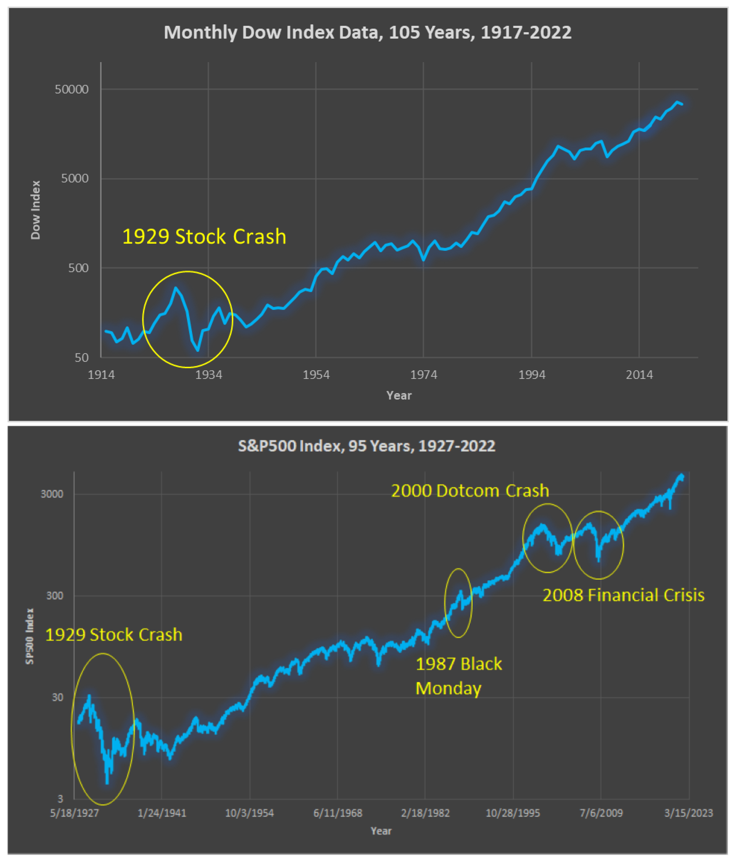

Figure 2.
(top) Example of Algorithm 1 in action, with a segment of the S&P500 data, showing key elements. When SMA(50) crosses below the SMA(200), the method switches from long to short or cash, and vice versa. (bottom) Performance of Alg1 vs. BnH, on SPX, 1982–2022. Alg1 underperforms simple BnH, but it reduces drawdowns. That in itself may be a benefit for small investors.

Figure 3.
Performance of more sophisticated algorithms on SPX and IXIC, still based on the same set of ideas, which deliver strong performance, yet limited and improving drawdowns. Since these time periods include several major market events, including the Black Swans, these results indicate that fairly elementary algorithms can indeed deliver powerful investment results, which may be applicable to both professional and individual small investors.

Figure 4.
The performance of SPX over the period 2020–2022 (top), IXIC (middle), and normalized indices (bottom) which facilitates comparisons. It is obvious from the normalized index figure (bottom) that SPX and IXIC are highly correlated, but that IXIC moves more (in technical jargon, it has a higher beta). It is interesting to note that for the full 3-year period 2020–2022, both indices actually ended up positive: SPX was up 17.9%, while IXIC was up 15.1%, which are certainly not bad returns for the simple BnH method over such a volatile period. However, the maximum drawdowns during the period were certainly distressing (33.9% for SPX, and 35.9% for IXIC). Can we do better?

Figure 5.
If the major indices SPX and IXIC had a rough ride during 2020–2022, just look at some popular stocks: (top) AMZN, (middle) NFLX, and (bottom) TSLA.
Figure 5.
If the major indices SPX and IXIC had a rough ride during 2020–2022, just look at some popular stocks: (top) AMZN, (middle) NFLX, and (bottom) TSLA.

Figure 6.
Performance of a FastHedge trading strategy for AMZN stock in the 3-year period 2020–2023, including portfolio gains as well as the trades made.
Figure 6.
Performance of a FastHedge trading strategy for AMZN stock in the 3-year period 2020–2023, including portfolio gains as well as the trades made.

Figure 7.
Performance of a FastHedge trading strategy for NFLX stock in the 3-year period 2020–2023, including portfolio gains as well as the trades made.
Figure 7.
Performance of a FastHedge trading strategy for NFLX stock in the 3-year period 2020–2023, including portfolio gains as well as the trades made.

Figure 8.
Performance of a FastHedge trading strategy for TSLA stock in the 3-year period 2020–2023, including portfolio gains as well as the trades made.
Figure 8.
Performance of a FastHedge trading strategy for TSLA stock in the 3-year period 2020–2023, including portfolio gains as well as the trades made.

Figure 9.
(top) The performance of a FastHedge algorithm on the Nasdaq index IXIC over a 40-year period ending 31 December 2022, compared to BnH. (middle) An indication of the investment position for each trading day, which shows the trades made by the system. (bottom) This system has robust performance, easily beating the index, while also reducing drawdowns significantly.

Figure 10.
(top) The performance of a FastHedge algorithm on the S&P500 index SPX over a 40-year period ending 31 December 2022, compared to BnH. (middle) An indication of the investment position for each trading day, which shows the trades made by the system. (bottom) This system has robust performance, easily beating the index, while also reducing drawdowns significantly.

Figure 11.
(top) The performance of a FastHedge algorithm for trading AAPL stock over a 40-year period ending 31 December 2022, compared to BnH. (middle) An indication of the drawdowns for the FastHedge algorithm over the 40-year period, and (bottom) of the BnH algorithm with AAPL stock, with unacceptably high losses above 80%.

Figure 12.
(top) The performance of a FastHedge algorithm for trading AAPL stock with 1.4X leverage (when long) over a 40-year period ending 31 December 2022, compared to BnH (plotted without leverage). (middle) An indication of the drawdowns for the FastHedge algorithm over the 40-year period, and (bottom) of the 1.4X leveraged BnH algorithm with AAPL stock, with catastrophic losses nearing 100%.

Figure 13.
Tabular representation of key findings of this paper, showing performance over a range of trading time periods: approximately 5 months, 1 year, 3 years, 10 years, and 40 years, all ending 31 December 2022, for a various of financial instruments, including indices and individual stocks.
Figure 13.
Tabular representation of key findings of this paper, showing performance over a range of trading time periods: approximately 5 months, 1 year, 3 years, 10 years, and 40 years, all ending 31 December 2022, for a various of financial instruments, including indices and individual stocks.

Figure 14.
Tabular representation of key findings of this paper, showing the performance of all tested financial variables over long time horizons, and quantified using a variety of metrics, including the ARM Ratio, the PARC Measure, and the Sharpe Ratio. This table provides strong evidence that both the ARMR and PARC outperform the Sharpe Ratio, with PARC taking the top spot, as useful metrics for investment decisions. Tellingly, even when the leveraged AAPL stock has a 99.8% MaxD, Sharpe still gives it a fairly high score of 0.612, while ARMR downgrades it considerably to 0.189, and PARC grades it simply as 0.000, its minimum score. Among investments that were tested for long periods (9 K–10 K days), our highlighted investment in IXIC performs best according to PARC (and visually has an excellent performance in Figure 9), and is thus our baseline strategy. More details of comparisons are provided in the text.

Figure 15.
Performance of the suite of FastHedge algorithms on the IXIC index over the 10,000 trading days (about 40 years) ending 31 December 2022. The core settings used here are slightly different than those used in Figure 14, but our main point is that a large variety of the core algorithms performed very well, and had acceptable levels of maximum drawdowns. Furthermore, each of these algorithms was held fixed (including all other parameters) during the entire test. Moreover, the design of these algorithms is entirely generic, and they have not been tuned to any financial variable or time period. This is strong evidence against any charge of algorithm overfitting or data mining in our framework. Only a few of the algorithms actually underperform the IXIC index itself, and for reasons we understand fully. (No. 1 is the basic BnH, and does the worst.)

Disclaimer/Publisher’s Note: The statements, opinions and data contained in all publications are solely those of the individual author(s) and contributor(s) and not of MDPI and/or the editor(s). MDPI and/or the editor(s) disclaim responsibility for any injury to people or property resulting from any ideas, methods, instructions or products referred to in the content. |
© 2023 by the author. Licensee MDPI, Basel, Switzerland. This article is an open access article distributed under the terms and conditions of the Creative Commons Attribution (CC BY) license (https://creativecommons.org/licenses/by/4.0/).
Share and Cite
MDPI and ACS Style
Topiwala, P. Surviving Black Swans II: Timing the 2020–2022 Roller Coaster. J. Risk Financial Manag. 2023, 16, 106. https://doi.org/10.3390/jrfm16020106
AMA Style
Topiwala P. Surviving Black Swans II: Timing the 2020–2022 Roller Coaster. Journal of Risk and Financial Management. 2023; 16(2):106. https://doi.org/10.3390/jrfm16020106
Chicago/Turabian StyleTopiwala, Pankaj. 2023. "Surviving Black Swans II: Timing the 2020–2022 Roller Coaster" Journal of Risk and Financial Management 16, no. 2: 106. https://doi.org/10.3390/jrfm16020106