Abstract
This study constructs Divisia monetary aggregates for the “Asian Tigers”—Hong Kong (1999–2024), South Korea (2009–2024), Singapore (1991–2021), and Taiwan (2005–2024)—and assesses whether Divisia monetary aggregates explain nominal GDP better than simple-sum money. Our findings demonstrate that Divisia indices respond more sensitively to economic shocks. For Hong Kong and Taiwan, narrow Divisia money provides the best explanations for fluctuations in nominal GDP. Our results suggest that Divisia monetary aggregates can be beneficial for monetary policy analysis in these territories and underscore the importance of further research into the empirical performance of Divisia monetary aggregates in macroeconomic prediction.
1. Introduction
The “Barnett critique” highlights the superiority of Divisia monetary aggregation over the traditional simple-sum method of monetary aggregation (Barnett et al. 1992; Chrystal and MacDonald 1994; Belongia 1996). The simple-sum approach, which assumes that all financial components are perfect substitutes, is not consistent with economic theory. Even much earlier studies (Chetty 1969; Moroney and Wilbratte 1976; Boughton 1981) found that financial assets are less than perfect substitutes and advocated for different weights to be assigned to each component within monetary aggregates. While the simple-sum method has historically been used to measure spikes in the growth rate of the money supply, Barnett (2016) has demonstrated that these simple-sum spikes can be misleading. For example, after the end of the “monetarist experiment period”, Milton Friedman observed a seemingly alarming surge in simple-sum M2, which Barnett attributed to regulatory changes having no significant effect on the demand or supply for monetary services in the economy. Barnett’s research highlights that the Divisia index, based on well-established aggregation and index number theory, offers a more accurate measure of the money supply by avoiding the distortions and unusual spikes that are inherent in the simple-sum method.
The survey by Kumah (1989) indicated that the measurement of money in over 150 countries is limited to M1, M2, and M3, depending on the level of development or monetization of the financial system. A comparison of M2 and Lf (which is similar to M3 in other countries), and inflation rates in South Korea (hereafter Korea) from January 1998 to September 2022 reveals that these traditional simple-sum monetary aggregates could not adequately reflect the inflation trend or nominal GDP during the same period. This observation underscores Barnett’s (1980) criticisms of adding financial assets’ components without appropriately weighing each asset’s contribution to the monetary service flow. Barnett argued that the simple-sum monetary aggregate, which assumes equal weights for all components, cannot accurately measure the flow of monetary services. He advocated the well-known Divisia quantity index, which weights component growth rates with the value shares for each component, to provide a measure consistent with economic aggregation and index number theory.
The superiority of the Divisia monetary aggregates has been increasingly recognized across many countries. Studies have shown that the Divisia aggregates provide better recession signals, more accurate money-demand predictions, and improved macroeconomic forecasts for the Euro Area and the United States (Hendrickson 2014; Serletis and Gogas 2014; Barnett and Gaekwad 2021; Brill et al. 2021). In Asia, Divisia aggregates have been found to offer more precise monetary signals during financial crises and better forecasts of economic activity, particularly in Singapore, India, and China, although their efficacy during the COVID-19 pandemic posed challenges (Barnett and Nguyen 2021; Barnett et al. 2022b; Sengupta et al. 2024). Further confirmation of the Divisia monetary aggregates’ utility in enhancing monetary policy comes from studies in the UK and Saudi Arabia (Alkhareif and Al-Rasasi 2021; Belongia and Ireland 2021; Barnett et al. 2022a). Since 2010, research in territories like Germany, Indonesia, Israel, Pakistan, Taiwan, and Turkey supports the advantages of the Divisia aggregates (Sarwar et al. 2010; Puah and Hiew 2011; Chen and Nautz 2015; Benchimol 2016; Binner and Kelly 2017; Polat 2018). However, relevant studies about Korea, Taiwan, Hong Kong, and Singapore have become less common in recent times (See Appendix A Table A1).
In light of this fact, active research on Divisia monetary aggregates in various Asian countries is now underway (Jha and Longjam 2008; Barnett and Nguyen 2021). However, there has been a noticeable gap in research for Hong Kong, Korea, and Taiwan—territories that continue to use simple-sum monetary indicators. The only previously published research on Divisia monetary aggregates for Taiwan was Shih (2000), who constructed Divisia monetary aggregates for Taiwan and evaluated the empirical performance of those aggregates against the standards chosen by the central bank for the intermediate target variable in the conduct of monetary policy. Additionally, such research on Hong Kong, Korea, and Taiwan could enable a meaningful focus on applying Divisia monetary aggregates to all developing and developed Asian territories. Habibullah (1999) states that the Divisia monetary aggregates are more effective in developed countries with market-oriented financial systems. Korea’s recent reclassification as a developed country by the United Nations Conference on Trade and Development (UNCTAD) in July 2021 highlights the need to examine the usefulness and feasibility of Divisia monetary aggregates in this new context.
The term “Asian Tigers”, also known as “Asian Dragons”, collectively refers to Hong Kong, Korea, Singapore, and Taiwan, which experienced rapid economic growth from the 1960s to the 1990s (Figure 1). This term metaphorically compares these territories’ dynamic and aggressive economic growth to the characteristics of tigers. There are two main reasons why our study focuses on the Asian Tigers. First, despite their high level of economic development, these territories still use simple-sum monetary aggregates and can benefit from exploring the Divisia approach. Second, the complexity and advanced nature of these territories’ financial systems make them highly relevant for observing the effects of Divisia monetary measurement. For these reasons, research on Divisia monetary aggregates for the Asian Tigers is likely to provide significant academic and policy implications.
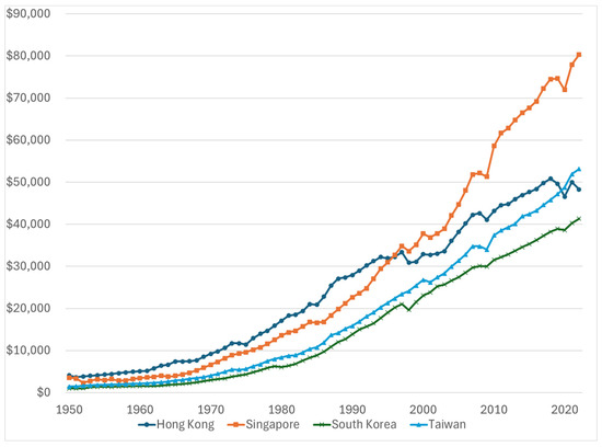
Figure 1.
Nominal GDP per capita of the Asian Tigers (1950–2022). Source: Bolt and Van Zanden-Maddison Project Database 2023. Note: These data are adjusted for inflation and differences in the cost of living and are expressed in international dollars at 2011 prices.
Our study aims to calculate and compare Divisia monetary aggregates with simple-sum aggregates for the Asian Tigers—Hong Kong, Korea, Singapore, and Taiwan. To achieve this, we utilize relevant data for each country’s money supply and conduct a comparative analysis between the simple-sum and Divisia monetary aggregates. The study addresses two key research questions. First, can countries achieve more accurate analytical research outcomes using Divisia economic monetary aggregates instead of simple-sum accounting aggregates? Is Habibullah’s (1999) conclusion still relevant in the current economic environment? Second, do Divisia economic monetary services provide a better explanation of nominal GDP than simple-sum accounting measures of money? By exploring these questions, the study aims to enhance the understanding of the relevance and effectiveness of Divisia measures in varying economic contexts.
This study has three significant contributions and implications. Firstly, it is the only study on economic monetary aggregation that collectively focuses on the Asian Tigers, known for their rapid economic growth. Notably, there has been no research on Korea and Taiwan since 2010, and no studies have examined the Divisia monetary aggregates in Hong Kong. Secondly, this study provides an opportunity to examine whether Divisia monetary aggregates can effectively reflect economic conditions in developed Asian territories. Finally, this study will provide a more accurate financial policy indicator for these Asian territories.
For example, (Barnett et al. 2022b) highlight the importance of the Divisia index for monetary aggregation in Hong Kong, particularly with the emergence of Central Bank Digital Currencies (CBDCs) and the increasing diversity of transaction services. In the case of Korea, the Bank of Korea emphasized the significance of Divisia monetary aggregates in a note (Park and Shim 2018), demonstrating that the Divisia economic index for M2 provides a more accurate reflection of economic growth than the simple-sum accounting monetary aggregate. Furthermore, the Korea Institute of Finance argued that “For quantitative easing (QE) to be successful in the post-global financial crisis era, it is important to measure the actual liquidity that can influence the real economy, which Divisia monetary aggregates can help achieve” (Korea Institute of Finance 2016). In the case of Taiwan, the rapid economic, social, and political changes since the early 1980s led to long-term macroeconomic imbalances. The subsequent financial innovations and deregulation, particularly following the 1989 Banking Act amendment, revealed the limitations of the simple-sum method for measuring money supply, necessitating the adoption of the Divisia index (Binner et al. 2002). Furthermore, Shih (2000) suggests that a re-evaluation of the usefulness of Divisia aggregates as a monetary target variable after the developments of the Taiwanese financial markets reach a certain stage, might be useful. These studies underscore that Divisia monetary aggregates provide a more reliable tool for informing financial policy.
In sum, this study pioneers research on the Asian Tigers jointly, evaluating the effectiveness of Divisia monetary aggregates across various economic contexts and emphasizing their importance as a more accurate financial policy indicator.
We hypothesize that the Divisia monetary index provides a more accurate and robust explanation of nominal GDP fluctuations than the simple-sum method. The Divisia monetary index, by accounting for the different levels of services of various monetary assets, is expected to outperform the traditional simple-sum method in explaining changes to nominal GDP. To test this hypothesis, we comprehensively compare the Divisia economic monetary index with the simple-sum accounting measure across the Asian Tiger territories to assess the effectiveness of the measures in explaining nominal GDP. Specifically, we use the Augmented Dickey–Fuller (ADF) test to check for stationarity, the Johansen cointegration test to analyze long-term relationships, and the Vector Error-Correction Model (VECM) to examine both short-term dynamics and the long-term equilibrium. The objective is to determine whether the Divisia monetary index indeed offers a superior explanation of nominal GDP fluctuations than the simple-sum aggregate.
The remainder of this paper is structured as follows: Section 2 outlines the methodology followed for our analysis, while Section 3 presents the data and identification strategies used for analyzing the issue. Section 4 details the results of the Divisia monetary aggregates and the corresponding test outcomes. Finally, Section 5 discusses the limitations and concludes the study.
2. Methodology
2.1. Simple Sum
Problems with the U.S. monetary demand function using simple-sum money measures were caused by rapid institutional innovation and changes in regulations. Liberalizations of bank management have caused demand for the constituent assets of the available simple-sum monetary accounting aggregates to fluctuate. The mix of monetary services from monetary assets and the savings motive associated with the interest rate payments on monetary assets has varied across components and over time. The opportunity costs of each monetary asset have fluctuated over both time and monetary assets. Measuring the services from aggregated monetary assets by simple-sum aggregation has become inconsistent with aggregation and index number theory and produces the appearance of instability of the demand from the improper measurement of the service flow.
Barnett (1980) identified the fundamental problem in measuring the monetary service flow as an accounting sum. He pointed out that monetary aggregation by accounting summation implies that each component asset is a perfect substitute for each of the others, and he showed how existing economic aggregation and index number theory can solve the problem. In addition, numerous studies have argued that the assumption of perfect substitutability is unreasonable (e.g., Feige and Pearce 1977; Barnett 1982).
Fisher (1922) concluded that the simple sum is the most unreasonable among all the possible indexes he studied in his famous book (also see Barnett et al. 1992). As stated by Fisher (1922, p. 363), the simple sum has the two worst properties of an index number:
“There are two objections to Formula 1, the simple arithmetic (1) that it is simple and (2) that is arithmetic; that it is at once freakish and biased.”
Barnett (1980, 1981) provided the relevant microeconomic aggregation and index number theory to measure monetary services. See (Barnett et al. 1992) for an overview of the relevant derivation and theory.
2.2. Divisia Index
In Divisia aggregation, the opportunity costs of individual monetary asset services are the prices used in computing the share weights of the monetary component growth rates. This opportunity cost is the user cost price of each monetary asset’s services. That price is the interest rate foregone to consume the services of the asset during the period. The interest foregone at the end of the period is discounted from the end of the period to the beginning of the discrete time period (Barnett 1978). Thus, the opportunity cost is
where is the expected rate of return on the ith component monetary asset, and R refers to the expected return on the “benchmark” asset, which is an economy’s pure capital providing only store of value and no other services. For example, demand deposits and cash that do not pay interest have the highest user cost price with = 0 and, hence, the highest marginal utility. But as in the famous diamonds versus water paradox, high marginal utility does not necessarily mean high total or average utility. While the user cost prices are needed to compute the expenditure shares that weigh the component growth rates, the user cost prices are not weights in the index. They are prices at the margin. In aggregation and index number theory, user cost price aggregates have a dual relationship with monetary quantity aggregates and can be used to produce the implied interest rate aggregates uniquely (Barnett 2010).
Upon deriving the user cost of monetary assets, Barnett (1980) linked the resulting index number theory with microeconomic monetary aggregation theory. Diewert (1976) defined a class of superlative index numbers that bridged the gap between index number theory and aggregation theory. Diewert proved that the Fisher Ideal and Törnqvist–Theil Divisia indices are in a class of superlative indexes providing a second-order approximation to any aggregator function. Barnett correspondingly proposed two quantity indices for monetary aggregation, consisting of the Fisher Ideal and Divisia indices in discrete time with user cost prices. The Törnqvist–Theil discrete time approximation to the Divisia index is the most useful quantity index for policymakers since it has the most easily understood form of any index numbers in Diewert’s (1976) superlative index number class. We shall hereafter refer to the Törnqvist–Theil as just the Divisia index, although, strictly speaking, the Divisia index is the continuous time index attained when discrete time converges to continuous time. Ishida (1984) correspondingly agreed that the Divisia index (in discrete time) is the best statistical index, and he then proceeded to produce Divisia monetary aggregates for Japan.
The Divisia index in continuous time is a line integral approximated during time period t in discrete time by the Törnqvist–Theil index, . Let designate the multiplication operator over the N component assets, i = 1, …, N. Then, the resulting discrete-time Divisia index is
where xi,t is the quantity of good i during period t. In our case, that quantity will be the nominal quantity of monetary asset i, and sit will be asset i’s share in the user cost evaluated expenditure on the services of all of the N monetary asset components, as follows:
Taking the log of each side of Equation (2), we find the equation below and can observe that the growth rate of the Divisia index is a weighted average of the growth rates of each component asset, as follows:
The growth rate of the Divisia aggregate can be written as
where and is the log change operator. Single-period changes, beginning with a base period, could be cumulated to determine the Divisia aggregate level in each period.
2.3. Benchmark Rate
The benchmark rate is an important variable in the user cost prices needed in the computation of the expenditure shares appearing in the Divisia index growth rate. The benchmark rate theoretically reflects the return on a pure capital investment that offers no monetary services, setting an upper limit on the returns on monetary assets that do provide monetary services, as well as a possible lower rate of return. The benchmark rate must never be less than the highest return among the component assets, which provide both monetary services as well as investment returns. In practice, the benchmark rate is often calculated as the highest yield among the assets in the broadest monetary aggregate, or a proxy yield on a high-yielding illiquid asset. The benchmark rate must never be less than the rate of return on any of the monetary component assets to avoid negative user cost prices violating the definition of the benchmark asset.
Selecting an appropriate proxy for the benchmark rate is essential, as it significantly impacts the behavior and accuracy of Divisia monetary aggregates. Countries tailor this concept to their specific contexts. For instance, Hahm and Kim (2000), for Korea, opted for the upper envelope over the yields on 3-year corporate bonds and the yield on all monetary assets, while Barnett and Nguyen (2021) used the prime lending rate in Singapore. In Taiwan, Binner and Kelly (2017) added a 100-basis point liquidity premium to the upper envelope over the rates of return on all monetary assets within the aggregate. The choice of proxy is important to ensure that the user costs accurately reflect the opportunity costs of holding money and align with the financial environment of the respective country. However, there is reasonable robustness of the Divisia index to the choice of benchmark rate, since that rate appears symmetrically in all terms in both the numerator and denominator of the expenditure shares. In contrast, accurate measurement of the rates of return on the component assets is very important, since the share weights are sensitive to those measures.
2.4. Vector Error-Correction Model (VECM)
Based on our results, we evaluate whether Divisia monetary aggregates significantly enhance the explanatory power of changes in nominal GDP (NGDP) compared to simple-sum aggregates. To test this hypothesis, we first verify the order of integration for each of the variables using the Augmented Dickey–Fuller (ADF) test to check for unit root, with the lag lengths determined by the Akaike Information Criterion (AIC) (Akaike 1973). The null hypothesis is that the variable has a unit root. Two variables are cointegrated if there exists a linear combination that is integrated of order zero, I(0), which indicates that the variables have a long-run relationship and share a common stochastic trend over time (Engle and Granger 1987). Cointegration requires that the variables be stationary in their first differences and non-stationary in levels. Based on the findings of the ADF test, we then assess cointegration using the Maximum Likelihood approach proposed by Johansen (1988).
Following these steps, we use the Vector Error-Correction Model (VECM) to analyze whether Divisia monetary aggregates offer a better explanation for NGDP, a widely accepted proxy for economic activity, compared to the simple-sum monetary aggregates. The VECM is particularly suitable for addressing the limitations of the Vector Autoregressive (VAR) model, specifically its inability to account for cointegrated variables that share a long-term equilibrium relationship. This framework allows us to model both short-term deviations and long-term equilibrium relationships between variables. Previous studies have used similar approaches, employing the ADF test and estimating models with ECM or VECM techniques to assess the explanatory power of Divisia monetary aggregates (Habibullah 1999; Hahm and Kim 2000; Sarwar et al. 2010; Ramachandran et al. 2010; Puah and Hiew 2011; Bhatnagar 2022). The VECM is formulated as follows:
where L is the lag operator, Mt refers to the respective variable for monetary policy for the four territories (that include simple-sum monetary aggregates, Divisia monetary aggregates, and an interest rate variable), and NGDPt is the log of quarterly nominal GDP, while (NGDPt−1 − Mt−1) refers to the error-correction term. Following Ramachandran et al. (2010), we test the null hypothesis that β13 = 0 and β23 = 0. If we reject the first and accept the second, then that would imply that the growth rate of output responds to disequilibrium errors in the last period, while the growth rate of money does not.
2.5. Forecast Error-Variance Decomposition (FEVD)
We use a Forecast Error-Variance Decomposition (hereafter referred to as FEVD) analysis to quantify the importance of each shock in explaining the variation in each variable by calculating the fraction of the forecast error variance attributable to each shock at different horizons. This analysis provides insights into the dynamic interactions between variables, revealing the relative importance of various shocks in driving fluctuations.
In the context of monetary policy analysis, FEVD has proven particularly valuable. For instance, when applied to Divisia monetary aggregates, FEVD can demonstrate their superior performance over simple-sum aggregates in explaining variations in economic output. The analysis effectively identifies which monetary aggregates influence output more, underscoring their value in policy analysis. The ability of FEVD to decompose and attribute forecast errors to specific shocks makes it an especially valuable tool for understanding the nuances of monetary policy and economic fluctuations, thereby informing more effective decision-making.
3. Data
3.1. Hong Kong
Hong Kong’s financial system is structured around a three-tier banking framework comprising licensed banks, restricted license banks (RLBs), and deposit-taking companies (DTCs). Licensed banks, offering the broadest range of services, significantly influence the narrow money supply (M1) through demand deposits and currency circulation. RLBs principally engage in merchant banking and capital market activities and take deposits of any maturity of HKG 500,000 or more. DTCs contribute to broader monetary aggregates, particularly M2 and M3, by accepting deposits of HKG 100,000 or more with an original term of maturity of at least 3 months. DTCs also engage in a range of specialized activities, including consumer finance, commercial lending, and securities business.
Significant fluctuations have marked the trajectory of Hong Kong’s monetary aggregates following domestic policy changes and external economic pressures. During the 1980s and early 1990s, Hong Kong saw steady growth as it established itself as a global financial center. However, the 1997 Asian Financial Crisis introduced volatility, leading to stringent monetary policies to defend the currency peg and stabilize the financial system. Post-1997, especially after the 2008 global financial crisis, broader monetary measures such as M2 and M3 expanded again from liquidity injections by the Hong Kong Monetary Authority (HKMA) and increased foreign capital inflows.
The monetary aggregates M1, M2, and M3 are primary indicators of the economy’s money supply. Appendix B Table A2 provides a basic description of Hong Kong’s monetary asset components. The monthly dataset covers January 1999 to June 2024, with the data on levels reported in millions of Hong Kong dollars (HKG). M1, the most liquid form, reflects immediate spending power through currency in circulation and customers’ demand deposits. M2 builds upon M1 by including customers’ savings and time deposits and negotiable certificates of deposit (NCDs) issued by licensed banks held outside the banking sector, offering a broader perspective on available funds. M3 encompasses all components of M2 plus customers’ deposits with restricted license banks and deposit-taking companies, plus NCDs issued by these institutions held outside the banking sector.
The types of liabilities included in the money supply of Hong Kong are similar to those in other economies. However, a major difference relates to the treatment of Government and Exchange Fund placements with banks. The government’s deposit holdings are included in the Hong Kong dollar broad money, whereas in most other economies, they are excluded. Furthermore, exchange fund placements with a maturity of over 1 month are counted as customer deposits and, hence, included in the money supply figures.
Although the HKMA reports interest rates for savings and time deposits with licensed banks, the HKMA does not provide the rates for savings and time deposits with restricted licensed banks and deposit-taking companies. We use the average interest rates for time deposits (6 months) and savings deposits of less than HKG 100,000 quoted by the major licensed banks for time and savings deposits included in M2. But for deposits with RLBs and DTCs, we use the 3-month time deposit rate, since DTCs require that deposits have an original term of maturity of at least 3 months. However, due to data limitations, although DTCs require the deposits to be of at least HKG 100,000, and RLBs require the deposits to be of at least HKG 500,000, we use the 3-month deposit rate for deposits of less than HKG 100,000 as a proxy for the rate of deposits with RLBs and DTCs.
In the series for the level of NCDs issued by RLBs and DTCs during the period from May 2011 to April 2015, the quantities reported are zeros, which does not seem credible. We smoothed the data on NCDs for the above period by approximating the zero-quantities by the average of the quantities 12 months before and 12 months after that period. Since the rate of return on NCDs is not reported, we use the yield for 1-year exchange fund bills, which has been included in the broad money aggregates since April 1997. We chose a timeline post-1997 to make use of the “new data” series reported by HKMA. For the benchmark rate, we use the best lending rate quoted by the Hong Kong and Shanghai Banking Corporation Limited and reported by the HKMA.
To compare the performance of Divisia monetary aggregates and simple-sum aggregates in explaining nominal GDP, we use the seasonally adjusted data for nominal GDP between 2009 Q1–2023 Q4 reported by the Census and Statistics Department of the Government of the Hong Kong Special Administrative Region. For the interest rate variable, we use the overnight lending rate provided by HKMA. For our analysis, we use log-transformed variables unless mentioned otherwise. We seasonally adjust all the monetary variables using the X-13 ARIMA (Autoregressive Integrated Moving Average) SEATS procedure.
3.2. South Korea
In Korea, the compilation of various monetary indicators, including the old version of M2, began in March 1981. In 2002, the Bank of Korea revised and published M1 and M2 as new indicators, guided by the IMF’s Monetary and Financial Statistics Manual (International Monetary Fund 2000). Since 2006, the Bank of Korea has also prepared and published liquidity indicators Lf and L, resembling M3 and M4 in some other territories. The monetary statistics by economic entities, released in September 2013, show the amount of currency held by each economic entity based on M2 among monetary and liquidity indicators. Until 2002, Korea’s monetary and liquidity indicators served as intermediate targets for monetary policy. However, with the adoption of an inflation-targeting system, the interest rate-oriented monetary policy framework now uses interest rates as informative variables for policy management.
Appendix B Table A3 provides a basic description of Korea’s monetary asset components, covering a monthly dataset from January 2009 to June 2024, with the data on levels reported in millions of Korean won (KRW). The data, sourced from the Economic Statistics System (ECOS) of the Bank of Korea, are based on monthly averages and have been seasonally adjusted. The Bank of Korea classifies the primary components of M1 (narrow money) as currency in circulation, demand deposits, and transferable savings deposits. M2, which includes M1, refers to broad money, encompassing money market funds (MMFs), short-term time and savings deposits, beneficiary certificates, marketable financial instruments, short-term financial debentures, short-term money in trust, and others. The maturity of all assets in M2 is within 2 years. Lf includes liquid financial instruments. L includes long-term assets (over 2 years), such as long-term financial instruments and life insurance reserves.
Unfortunately, the Bank of Korea does not report matched interest rates for all assets1. When the Bank of Korea collects data, it gathers total amounts and interest rates separately from various institutions, which can lead to mismatches between the two2. For instance, short-term financial debentures and short-term money in trust do not have corresponding interest rates. In such cases, to best reflect the interest rates of short-term assets, the most relevant proxy interest rates were used, such as the interest rates of 1-year treasury bonds and 91-day CDs, which best capture the characteristics of short-term assets. For Lf’s life insurance reserves, the 3-year treasury bond rate was used as a proxy for the interest rate on life insurance because treasury bond yields are directly employed in insurance product design, pricing, and reserve calculations, and they also serve as a key factor influencing the overall financial performance of insurance companies (Lee 2016)3. L includes long-term assets such as liquid financial instruments like government and municipal bonds. In this case, to adjust for the yield curve, the rate of return on long-term assets was replaced with the interest rate on comparable short-term assets, specifically the 1-year Treasury bond rate.
This paper will use the corporate bond rate (BBB-) as the benchmark rate for Korea, following the approach of Hahm and Kim (2000) for compatibility with their results. However, there are two more reasons. First, there are data limitations for Korea. Barnett et al. (2013) measured the benchmark rate as the weighted average effective loan rate for low-risk, 31–365 days’ loans across all commercial banks from the FRED database maintained by the St. Louis Federal Reserve Bank. A comparable loan rate does exist in Korea and typically exceeds deposit interest rates. However, the loan rate is a weighted average rate for all loans, not specifically for low-risk short-term loans. Therefore, in the case of Korea, it is challenging to distinguish between various risk levels and loan periods. Secondly, corporate bonds in Korea are categorized by ratings such as AA- and BBB-, which allows for a more precise differentiation of risk levels. Moreover, the Bank of Korea provides data on corporate bonds with a 3-year maturity, which will be used in this study. While a 3-year bond rate is relevant to the theory, we do not use long-term bond rates, which would be too far removed from the necessary short-term rate of return for an accurate benchmark.
To compare the performance of Divisia monetary aggregates and simple-sum aggregates in explaining nominal GDP, we use the seasonally adjusted data for nominal GDP between 1999 Q1 and 2024 Q1 reported by the Federal Reserve Bank of St. Louis. For the interest rate variable, we use the overnight lending rate provided by the Bank of Korea. For our analysis, we use log-transformed variables unless mentioned otherwise.
3.3. Singapore
Singapore’s monetary policy framework employs an institution-based approach to measuring money supply, aligning with methodologies used in the United Kingdom and Germany. This approach defines monetary aggregates based on the liabilities of specific financial institutions rather than the characteristics of monetary instruments. The narrowest measure, M1, includes currency in active circulation and private sector demand deposits within the banking system. M2 expands upon M1 by incorporating quasi-money, while M3, the broadest measure, further includes net deposits with non-bank financial institutions (NBFIs). The banking system comprises the Board of Commissioners of Currency, Singapore (BCCS), and commercial banks, forming the foundation for M1 and M2 calculations. M3 extends this scope by integrating net deposits from finance companies, offering a more comprehensive view of the monetary landscape.
A significant modification to this framework, which has evolved over time, occurred in November 1998, following the Post Office Savings Bank’s (POSB) merger with the Development Bank of Singapore (DBS). This consolidation required a recalibration of monetary measurements, as POSB’s deposits were reclassified on par with other commercial banks and thus incorporated into M1 and M2 aggregates. Additionally, the computation of M3 was adjusted to include POSB’s term deposits held with the Monetary Authority of Singapore (MAS), which were previously excluded. To maintain consistency in monetary data, authorities implemented retrospective revisions dating back to October 1982, when POSB initially placed deposits with MAS. This restructuring underscores Singapore’s commitment to precise monetary statistics and adapting to evolving institutional dynamics. Consequently, Singapore’s monetary policy framework is anchored in a tripartite system of monetary aggregates—M1, M2, and M3—each serving as a distinct indicator of money supply with progressively expanding scope and complexity.
For Singapore, we use monthly data from January 1991 to June 2021, with data reported in millions of Singapore dollars (SGD) from the MAS. The period concludes in June 2021 due to the transition of the commercial bank interest rate data from monthly to quarterly reporting. The MAS reports three levels of simple-sum monetary aggregates. Appendix B Table A4 provides a basic description of Singapore’s monetary asset data. M1 includes currency in circulation and demand deposits in banks, both carrying zero interest rates. M2 expands upon M1 by adding fixed deposits, savings deposits, and negotiable certificates of deposit (NCDs) within the banking sector. M3 further broadens the definition of money by including net deposits in finance companies. According to MAS guidelines, POSB’s fixed deposits and savings deposits have been included within the respective commercial banks, while the remaining components of POSB have been incorporated into M1. Here, “banks” refers to commercial banks, and “finance” refers to finance companies.
Barnett and Nguyen (2021) previously examined Singapore’s financial data and proposed alternatives to address data limitations. Our paper not only refines their approach but also underscores the significant role of their proposals. To achieve a more accurate composition of monetary aggregates, POSB’s non-fixed deposits and non-savings components were included in M1, which aligns with Singapore’s banking guidelines. Following DBS’s acquisition of POSB in November 1998, POSB’s data were incorporated into M1 and M2, with separate data no longer provided. Consequently, M2 now includes POSB’s fixed deposits and savings, while M1 comprises the remaining components. The allocation of POSB data follows Barnett and Nguyen’s (2021) methodology, assuming POSB interest rates align with those of the banking sector.
For M3, net deposits with finance companies were divided into fixed and savings deposits using the net deposits’ liabilities ratio and corresponding 3-month interest rates. Due to the unavailability of the NCDS interest rate for M2, we substitute the 3-month T-bill rate. Barnett and Nguyen (2021) used the 3-month commercial bill rate but switched to the T-bill rate post-2013 after the MAS ceased providing the former data. The 3-month T-bill rate is chosen as it is a short-term, low-risk asset with comprehensive data available.
This paper adopts the short-term lending rate as the benchmark rate for Singapore, following the methodology of Barnett et al. (2013), for three principal reasons. First, from a theoretical perspective, the benchmark rate should reflect the rate of return on pure capital and must exceed the returns on all monetary assets that provide services to depositors. Second, from an economic standpoint, it is unrealistic for banks to offer deposit rates that exceed their investment yields. Lastly, in the specific context of Singapore, the prime lending rate consistently exceeds the interest rates on the component monetary assets.
To compare the performance of Divisia monetary aggregates and simple-sum aggregates in explaining nominal GDP, we use the seasonally adjusted data for nominal GDP between 2005 Q4 and 2020 Q2 as reported by the Singapore Department of Statistics. For the interest rate variable, we use the overnight lending rate provided by the Monetary Authority of Singapore. Due to the interest rates being reported from 2005 to 2020, we choose that timeline. For our analysis, we use log-transformed variables unless mentioned otherwise.
3.4. Taiwan
Taiwan’s financial system, while sharing similarities with other advanced economies in East Asia, possesses distinct characteristics that set it apart. The system is characterized by a well-developed banking sector and a robust regulatory framework. The Central Bank of the Republic of China (Taiwan), the nation’s central bank, plays a pivotal role in regulating monetary aggregates. These aggregates are essential indicators of the economy’s money supply and financial stability, and the central bank’s management of them is a key aspect of the financial system’s stability.
A unique feature of Taiwan’s financial landscape is the role of Chunghwa Post, the official postal service. Beyond its traditional functions, Chunghwa Post operates a postal savings system, forming a significant component of the nation’s broader financial infrastructure. This system allows individuals to hold savings accounts and make deposits, contributing substantially to the overall monetary aggregates, particularly M2. Integrating postal services with financial functions provides Taiwan with a distinctive mechanism for mobilizing domestic savings and enhancing financial system stability.
Over time, Taiwan’s monetary aggregates have shown significant changes in response to both internal and external economic factors. The rapid industrialization of the 1970s and 1980s led to substantial increases in M1 and M2, followed by a period of stabilization in the 1990s as the economy matured. Global events, such as the 1997 Asian Financial Crisis and the 2008 Global Financial Crisis, prompted shifts in monetary strategy. The central bank responded by implementing various measures to manage liquidity and ensure financial stability. In the post-2008 era, the central bank has maintained a cautious approach, balancing economic stimulus with concerns about asset bubbles and inflation, resulting in moderate growth in monetary aggregates with occasional adjustments.
Appendix B Table A5 provides a basic description of Taiwan’s monetary asset components. The monthly dataset covers January 2005 to June 2024 with the data on levels presented in millions of New Taiwan dollars (TWD). In terms of monetary aggregates in Taiwan, the central bank distinguishes between M1A and M1B, with M1A representing currency in circulation, checking accounts, and passbook deposits, while M1B includes M1A plus passbook savings deposits. M2 expands on M1B by including savings deposits, time deposits, foreign currency deposits, postal savings deposits, negotiable certificates of deposit (NCDs), money market funds (MMFs), repurchase agreements, and government deposits.
The data on levels for MMFs provided by the central bank start from October 2004. Therefore, for our analysis, we use the data starting from January 2005 to June 2024. However, the data for MMFs have not been reported since May 2017. We use a regression of the series to fill in the missing data.
For the rates of return on passbook deposits, passbook savings deposits, time and savings deposits, and foreign currency deposits of commercial banks, we use the respective interest rates quoted by the Bank of Taiwan and reported by the central bank. For the rate of return on NCDs, we use the 91–180 days’ NCDs rate in the secondary market. For the rates of return on repurchase agreements, we use the 91–180 days’ repos rate on government bonds in the secondary market. Since the rates of return on MMFs are not reported, we use the overnight interbank loan rate. For the benchmark rate, we use the average base lending rate offered by the five major banks as published by the Central Bank of the Republic of China (Taiwan).
To compare the performance of Divisia monetary aggregates and simple-sum aggregates in explaining nominal GDP, we use the seasonally adjusted data for nominal GDP between 2005 Q1–2024 Q1 reported by the National Statistics, Republic of China (Taiwan). For the interest rate variable, we use the overnight lending rate provided by the Central Bank of the Republic of China (Taiwan). For our analysis, we use log-transformed variables unless mentioned otherwise. We seasonally adjust all the monetary variables using the X-13 ARIMA (Autoregressive Integrated Moving Average) SEATS procedure.
4. Results
4.1. Divisia Monetary Aggregates Results
4.1.1. Hong Kong
In Hong Kong, as shown in Figure 2a and Figure 3a, M1 and DM1 are identical, as is expected since they consist of the same components with zero interest rates, leading to identical user cost prices. However, a significant divergence exists between the narrower M1/DM1 and the broader M2 and M3 measures for both simple-sum and Divisia aggregates. Simple-sum measures of M2 and M3 are generally higher than their Divisia counterparts, suggesting that simple-sum measures overstate the quantity of monetary services in the economy.
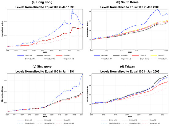
Figure 2.
Divisia versus simple-sum monetary aggregates for the four Asian tigers.
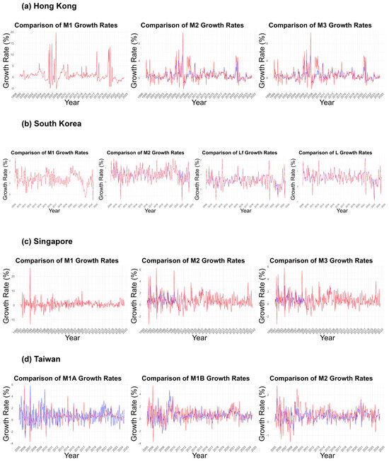
Figure 3.
Divisia versus simple-sum growth rates for the four Asian tigers.
Over time, particularly after 2008, the gaps between simple-sum and Divisia measures widen, likely due to financial innovations and interest rate changes. Divisia measures capture fluctuations, such as those during the global financial crisis and the COVID-19 pandemic, more distinctly, thereby highlighting their sensitivity to changes in the monetary environment. This underscores the importance of using Divisia aggregates for a more accurate understanding of monetary conditions in Hong Kong and the crucial role they play in shaping effective monetary policy.
4.1.2. South Korea
In Korea, as depicted in Figure 2b and Figure 3b, M1 and DM1 are almost identical, reflecting that M1’s components, including cash and demand deposits, have zero or very low interest rates. While there are slight differences between simple-sum M2 and DM2, with DM2 generally being slightly higher, the difference between them remains consistent over time.
A more noticeable difference is seen between Lf and DLf, with DLf being consistently higher. Additionally, DL follows a similar trend, maintaining a higher level than the corresponding simple-sum measures. Clearly, the broad simple-sum monetary aggregates undervalue the growth rate of monetary services produced by its components.
All monetary aggregates show an upward trend over time, with a notable increase after 2015. The consistent elevation of Divisia indices above simple-sum measures indicates that in Korea, the simple-sum measures undervalue the growth of monetary services in the economy, reflecting the structure of Korea’s financial market, interest rate environment, and financial instrument substitutability. Over time, the widening divergence between Divisia and simple-sum indices underscores the importance of using Divisia aggregates for accurate monetary policy analysis in Korea.
4.1.3. Singapore
In Singapore, Figure 2c and Figure 3c reveal notable differences between simple-sum and Divisia measures, especially in the broader aggregates such as M2 and M3. M1 and DM1 are nearly identical in Singapore, as the components of M1, such as currency and demand deposits, typically have low or zero interest rates, leading to equivalent user cost prices.
However, unlike in Korea where Divisia measures were consistently higher, Singapore’s DM2 and DM3 are slightly lower than their simple-sum counterparts, with nearly identical growth rates. This aligns with findings from Barnett and Nguyen (2021), that Divisia measures behave most differently from simple-sum measures when interest rates are high. A significant structural change in November 1998, when simple-sum M2 peaked due to the acquisition of POSB into the banking sector, is not reflected in Divisia’s measures, indicating their robustness to institutional changes not altering demand for monetary services.
During the 1997–1998 Asian financial crisis, a notable contraction in money services was observed in the growth rates of DM2 and DM3, while this change was less apparent in M2 and M3, thereby indicating that the Divisia index is more sensitive to economic shocks than the simple sum accounting stock.
4.1.4. Taiwan
In Taiwan, the analysis of monetary indicators, as shown in Figure 2d and Figure 3d, reveals significant differences between M1A and DM1A. Unlike other territories, Taiwan’s M1A includes passbook deposits that typically carry higher interest rates. In contrast, DM1A and DM2 show levels lower than their simple sum counterparts.
Over time, all monetary indicators exhibit an upward trend, although growth rates fluctuate during major economic events such as the 2008 global financial crisis and the 2020 COVID-19 pandemic. Divisia indices appear more sensitive to these shocks, and there is a trend of widening gaps between Divisia and simple-sum indices over time, reflecting the impact of financial innovations and interest rate changes.
The Divisia indices’ ability to capture changes in economic conditions more accurately underscores their importance in Taiwan’s monetary policy decisions. The differences between Divisia and simple-sum indices in M1B and M2 can be attributed to the structural characteristics of Taiwan’s financial market and the substitutability of various financial products. The greater sensitivity of Divisia indices to economic shocks and financial innovations suggests they provide a more accurate reflection of Taiwan’s monetary environment. The findings of this analysis significantly differ from the earlier paper by Shih (2000), as expected from the rapid development of Taiwan’s financial markets since the late 90s.
In sum, the analysis across Hong Kong, Korea, Singapore, and Taiwan demonstrates that Divisia monetary aggregates offer a more precise reflection of economic conditions than simple-sum measures, particularly during financial innovations and economic shocks. This is attributed to the Divisia indices’ heightened sensitivity to interest rate changes and their superior ability to capture the liquidity and substitutability of financial assets, underscoring their importance for accurate and effective monetary policy analysis in these regions.
4.2. VECM Results
4.2.1. Hong Kong
Appendix B Table A6 shows the results of the ADF test for all the variables in the log level and the first difference. The results show the presence of a unit root in the log level for all variables but no presence of a unit root in the first differences, thereby indicating that the order of integration of the variables is 1.
We then carry out the Johansen cointegration test using p − 1 lags, where p is determined by the Akaike Information Criterion (AIC). Based on the results, as presented in Appendix B Table A7, where “r” represents the cointegration rank, we conclude that at a 5% level of significance M1 and DM1 are cointegrated with NGDP. On the other hand, M2, DM2, M3, DM3, and R are not cointegrated with NGDP. We then proceed to fit a VEC model for M1 and DM1. Table 1 summarizes the results and Table 2 shows the results of the cointegration space. We note that in the cases of both M1 and DM1, we reject the null hypothesis that β13 = 0 and accept the null hypothesis that β23 = 0. This implies that the growth rate of both simple-sum and Divisia money are exogenous to NGDP and are, therefore, predictors of NGDP. In the case of Hong Kong, both simple-sum and Divisia aggregates perform equally well in terms of predicting NGDP. In Hong Kong, narrow money contributes towards the prediction of NGDP more significantly than broad money.

Table 1.
Error-Correction Term.
Table 2.
Results of the cointegration space.
4.2.2. South Korea
Appendix B Table A8 shows the ADF test results for all the variables at the log level and in the first difference. The ADF test results for Korea show that although GDP, M2, Lf, L, DM2, DLf, DL, and R are integrated to the order of 1, M1 and DM1 are not. They are in fact integrated in the order of 2. Because candidates for inclusion in a cointegrating vector must share an identical order of integration, we do not perform the Johansen cointegration tests for GDP and M1 and GDP and DM1. However, conducting the Johansen cointegration tests between GDP and the rest of the variables (M2, Lf, L, DM2, DLf, and DL) presented in Appendix B Table A9 shows no presence of cointegrating relationships.
4.2.3. Singapore
Appendix B Table A10 shows the ADF test results for all the variables at the log level and in the first difference for Singapore. The test results show that although M1, M2, M3, DM1, DM2, DM3, and R are integrated to the order of 1, NGDP is not. Because candidates for inclusion in a cointegrating vector must share an identical order of integration, we do not perform the Johansen cointegration tests for Singapore.
4.2.4. Taiwan
Appendix B Table A11 shows the results of the ADF test for all the variables at the log level and in the first difference. The results show the presence of a unit root in the log level for all variables but no presence of a unit root in the first difference, thereby indicating that the order of integration of the variables is 1.
We then conduct the Johansen cointegration test using p − 1 lags where p is determined by the Akaike Information Criterion (AIC). Based on the result, as presented in Appendix B Table A12, we conclude that at a 5% level of significance, DM1A is cointegrated with NGDP. On the other hand, M1A, M1B, M2, DM1B, DM2, and R are not cointegrated with NGDP. We then proceed to fit a VEC model for DM1A. Table 3 below summarizes the results, and Table 4 shows the results of the cointegration space. We note that in the case of DM1A, we reject the null hypothesis that β13 = 0 and accept the null hypothesis that β23 = 0. This implies that the growth rate of Divisia money supply is exogenous to NGDP and can, therefore, contribute to predicting NGDP. Similar to Hong Kong, in Taiwan, Divisia narrow money contributes more significantly towards the prediction of NGDP as opposed to broad money.
Table 3.
Error-Correction Term.
Table 4.
Results of the cointegration space.
4.3. FEVD Results
4.3.1. Hong Kong
Figure 4 and Figure 5 depict the variance decomposition for the models with M1 and DM1 in Hong Kong. The FEVD analysis confirms our findings above. We see that both M1 and DM1 are almost completely exogenous in the sense that almost none of their variances are being explained by shocks in NGDP. On the other hand, shocks in M1 and DM1 explain a significant fraction of the variances in NGDP. By the 10th quarter, those shocks explain almost 40% of the fluctuations in NGDP. It is important to note that, since the interest rates are zero for the components in M1, the simple sum and Divisia measures for narrow money in Hong Kong are the same. Therefore, the results of the FEVD analysis for M1 and DM1 are identical.
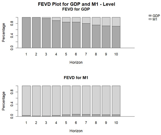
Figure 4.
FEVD Plot for GDP and M1.
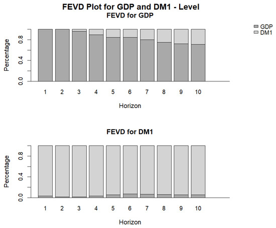
Figure 5.
FEVD Plot for GDP and DM1.
4.3.2. Taiwan
Figure 6 depicts the variance decomposition for the model with DM1A in Taiwan. We can see that DM1A is completely exogenous in the sense that almost none of its variance is explained by shocks in NGDP. On the other hand, shocks in DM1A explain a significant fraction of the variances in NGDP. By the 10th quarter, those shocks explain almost 40% of the fluctuations in NGDP.
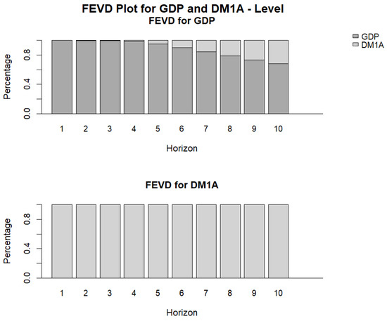
Figure 6.
FEVD Plot for GDP and DM1A.
4.4. Forecast Evaluation and Residual Analysis
4.4.1. Hong Kong
To check for the reliability of the Vector Error Correction model (VECM) used in Section 4.2, we perform a dynamic factor model and time-series analysis of the residuals. We backtest the VECM by producing Monte Carlo simulations with 1000 replications to forecast 10 horizons. We use the forecast performance metrics of mean absolute error (MAE), mean error (ME), and root mean square error (RMSE) for 10 horizons, shown in Appendix B Figure A1, to evaluate the model’s forecast performance. The MAE, ME, and RMSE all increase with the forecast horizon for both GDP and M1, with M1 consistently showing higher error rates. This suggests that the model’s predictions for money supply are less accurate than for GDP. The positive and increasing ME for both variables indicates a systematic overestimation in the model’s forecasts. Overall, the forecast performance for Hong Kong suggests that the VECM model’s accuracy diminishes for longer-term predictions, with money supply being particularly challenging to forecast accurately.
We then perform dynamic factor analysis as well as residual analysis on the VECM as shown in Appendix B Table A13. The factor loadings show that both GDP and M1 have equal weights on the first factor (PC1), while they have opposite weights on the second factor (PC2). This suggests that PC1 captures overall economic activity, while PC2 might represent divergences between GDP and money supply. The correlations between VECM residuals and factors are relatively low, indicating that the factors capture most of the systematic variation in the data. Residual diagnostics reveal normality, no significant correlation, and no volatility clustering. The analysis of GDP and DM1 are similar. Since the interest rates are zero for the components in M1, the simple sum and Divisia measures for narrow money in Hong Kong are the same.
4.4.2. Taiwan
Similarly, for Taiwan, we also present the forecast performance metrics of mean absolute error (MAE), mean error (ME), and root mean square error (RMSE) for 10 horizons, as shown in Appendix B Figure A2, to evaluate the model’s forecast performance. Taiwan’s VEC model demonstrates more stability and generally lower forecast errors compared to Hong Kong. The MAE initially increases but then slightly decreases for longer horizons, with GDP showing a higher MAE than DM1A. The ME is negative for both variables, indicating a tendency for the model to underestimate, though the bias for DM1A approaches zero at longer horizons. The RMSE increases with the forecast horizon, with GDP and DM1A showing similar patterns.
We then perform dynamic factor analysis as well as residual analysis on the VECM as shown in Appendix B Table A14. The factor loadings show that both GDP and DM1A have equal weights on the first factor (PC1), while they have opposite weights on the second factor (PC2). This suggests that PC1 captures overall economic activity, while PC2 might represent divergences between GDP and money supply. The correlations between VECM residuals and factors are relatively low except for that between the residuals of GDP and Factor 2, indicating that the factors capture most of the systematic variation in the data. Residual diagnostics reveal near normality, no significant correlation, and no volatility clustering.
5. Conclusions
A large number of theoretical studies as well as empirical studies have repeatedly shown that Divisia monetary aggregates are superior to their simple sum counterparts, which have no competent foundations in economic theory. Nevertheless, many central banks in the world, including those of developed economies, such as the Hong Kong Monetary Authority (HKMA), Bank of Korea (BOK), Monetary Authority of Singapore (MAS), and the Central Bank of the Republic of China (Taiwan), continue reporting money supply as a simple sum. This paper provides the construction of Divisia monetary aggregates jointly for the Asian Tigers, the four developed Asian economies, Hong Kong, South Korea, Singapore, and Taiwan, and explores the link between various monetary aggregates, interest rates, and output. Our analysis demonstrates that for developed Asian economies, Divisia monetary aggregates offer a more precise reflection of economic conditions than simple sum measures, particularly during financial innovations and economic shocks. Our analysis also suggests that for both Hong Kong and Taiwan, growth rates of Divisia monetary aggregates contribute to predicting nominal GDP. However, contrary to evidence in other advanced economies, such as the US, narrow money explains a larger fraction of the variance in economic activity than broad money.
Narrow money tends to respond more sensitively to short-term fluctuations in economic activity because narrow money is more directly and rapidly influenced by monetary policy in our sample. In contrast, broad money includes deposits and financial assets, which may be less sensitive to short run fluctuations, especially in economies where economic agents hold financial assets for longer-term purposes. For example, Friedman and Schwartz (1963) demonstrate how changes in the money supply impact economic activity differently over time, emphasizing the more immediate effects of narrow money. The higher explanatory power of narrow money in this sample may be due to monetary policy having a more pronounced and rapid effect on short-term cash and liquid assets, compared to financial assets held for longer durations in the Asian Tiger economies, perhaps for cultural reasons and slow subjective rates of time discount.
A significant portion of our analysis depended on data reported by the respective central banks of Hong Kong, South Korea, Singapore, and Taiwan. However, due to various limitations in data availability, we had to choose relevant proxy variables for certain interest rates, since the exact rates for the relevant variables included in the money supply of these territories were not reported by the respective central banks.
Author Contributions
All three authors contributed in major ways to this research. All authors have read and agreed to the published version of the manuscript.
Funding
This research received no external funding.
Data Availability Statement
All governmental sources clearly identified in the paper.
Acknowledgments
When relevant, acknowledgements mentioned in footnotes. We are truly grateful for the valuable feedback from the two anonymous reviewers.
Conflicts of Interest
The authors declare no conflicts of interest. All errors are our own.
Appendix A
Table A1.
Recent Country-specific Studies on Divisia Monetary Aggregates.
Table A1.
Recent Country-specific Studies on Divisia Monetary Aggregates.
| Authors | Country | Data Sources | Components | Years | Research Design | Main Results |
|---|---|---|---|---|---|---|
| Anderson and Jones (2011) | US | Federal Reserve Board, Bank Rate Monitor Corporation, FRED | M1, M2 | 1967–2011 | Divisia monetary aggregates, Revision of Monetary Services Indexes | Monetary services indexes (MSI) using Divisia monetary aggregation improves the accuracy of economic forecasts compared to simple sum aggregates, especially for broader monetary measures. |
| Barnett et al. (2022b) | China | People’s Bank of China, China Statistical Yearbook, Ant Group IPO prospectus, Alibaba China. | M0, M1, M2, M3 | 2000–2020 | Divisia monetary aggregates, Spectral analysis, Dickey–Fuller Test | Divisia aggregates outperform simple sums, especially for broader aggregates. Augmented Divisia captures COVID-19 effects. All aggregates have low short-run but high long-run coherence with GDP. Monetary aggregates lag GDP in the short run. |
| Barnett et al. (2016) | India | OECD database, Index Mundi, Econ Stats website, (Ramachandran et al. 2010) | M1, M2, M3 | 2000–2008 | SVAR analysis, Impulse response analysis, Variance Decomposition, Flip-Flop analysis, Forecasting | Models with Divisia monetary aggregates outperform those with simple sum aggregates in explaining exchange rate fluctuations and monetary policy impacts. |
| Belongia and Ireland (2022) | Euro Area | ECB, Bruegel | M1, M2, M3 | 2001–2019 | P-star regressions for the price level | Divisia monetary aggregates significantly predict inflation, with larger and statistically significant coefficients when the sample includes the COVID-19 pandemic period. |
| Belongia and Ireland (2021) | UK | Bank of England | Not applicable | 1978–2019 | P-star model, H-P filter | Divisia monetary aggregates provide a more stable framework for nominal income targeting under the zero lower bound. |
| Belongia and Ireland (2016) | US | Center for Financial Stability, Federal Reserve | M1, M2 | 1967–2013 | Structural VAR | Strong correlations between money supply measures and economic output/prices, especially when using Divisia monetary aggregates instead of simple-sum measures, suggest monetary policy plays an important role in business cycles. |
| Benchimol (2016) | Israel | Bank of Israel, Michelson and Suhoy (2014) | M1, M2 | 1995–2013 | New Keynesian DSGE models, Bayesian estimations, Simulations | Divisia monetary aggregates significantly impact output during crises, offer better forecasting accuracy, and money shocks predict financial risks. |
| Berar and Owladi (2013) | UK | Bank of England, Bankstats | Not applicable | 2011–2012 | Description of amendments to Divisia money series calculation | Switching the ISA interest rate in Divisia calculations from quoted to effective rates leads to downward revisions in Divisia money growth series, especially for the household sector. |
| Bhatnagar (2022) | India | Reserve Bank of India, Central Statistics Office | M1, M2, M3 | 1999–2019 | VECM, FEVD | Divisia aggregates with narrow money better predict economic activity compared to simple sum aggregates. |
| Binner and Kelly (2017) | Taiwan | Central Bank of the Republic of China (Taiwan), DataStream | M2 | 1985–2016 | Block recursive structural VAR model | Divisia monetary aggregates resolve short-run price, output, and exchange rate puzzles and provide sensible long-run impulse responses to monetary shocks. |
| Bissoondeeal et al. (2010) | UK | Bank of England Datastream | M1, M2 | 1977–2008 | Cointegration analysis, Maximum likelihood approach of Johansen and Juselius (1990) methods, Weak exogeneity tests, Parameter constancy tests | Long-run money demand relationships exist for UK Divisia and simple sum aggregates, with similar elasticities and minor differences in share price effects. |
| Brill et al. (2021) | Euro Area | ECB Statistical Data Warehouse, MFI | M1, M2 | 2003–2018 | Divisia monetary aggregates, Panel probit analysis | Divisia monetary aggregates for the euro area predict recessions more accurately than simple-sum aggregates and are useful for macroeconomic analysis and forecasting of country-specific monetary conditions. |
| Chen and Nautz (2015) | Germany | Deutsche Bundesbank, ECB, Eurostat, MFI | M3 | 2001–2014 | Divisia monetary aggregates, Structural VAR models, DM-test | The divergence between M3 and Divisia M3 provides superior forecasts for German output growth during the Great Recession compared to models using only M3 or Divisia M3. |
| Darvas (2015) | Euro Area | ECB, Bruegel, Eurostat | M1, M2, M3 | 2001- 2014 | Structural VAR models, Impulse response functions | Divisia monetary aggregates significantly impact output and prices, while simple-sum measures do not show significant results. |
| El-Shagi and Kelly (2013) | Euro area | Eurostat, IMF, ECB, NCB | M3 | 2003–2013 | Divisia monetary aggregates, Signals approach | Divisia aggregates are excellent predictors of debt crises, better capturing liquidity changes than simple sum measures. |
| Fleissig et al. (2023) | Euro Area | ECB | M1, M2, M3 | 2000–2021 | Fourier demand model, VAR models, Impulse response functions | Divisia monetary aggregates are robust to benchmark rates except during the global financial crisis, indicating differences from simple sum aggregates, particularly in elasticity and substitution responses. |
| Ghosh and Bhadury (2018) | India, Israel, Poland, the UK, the US | Bank of England, Bank of Israel, National Bank of Poland, Ramachandran et al. (2010), OECD database, Center for Financial Stability | M1, M2, M3, M4 | 1994–2017 | Unit root test, Var parameter stability test, Bootstrapped Granger causality | Strong causality from Divisia money to exchange rates, particularly when compared to alternative monetary indicators like simple sum aggregates or interest rates. |
| Gogas et al. (2019) | Euro Area | CEPR, Bruegel | M1, M2, M3 | 2001–2018 | Support Vector Machines | Divisia monetary aggregates significantly improve GDP forecasting accuracy compared to simple sum aggregates, demonstrating robust predictive power in various economic conditions and aggregation levels. |
| Hendrickson (2014) | US | Center for Financial Stability, St. Louis Federal Reserve FRED | M1, M2 | 1967–2012 | Cointegrated VAR model, Granger causality tests, Backward-looking IS equation, Dynamic New Keynesian model | Divisia monetary aggregates provide better explanatory power for money demand stability, nominal income, price level, and the output gap compared to simple sum aggregates. |
| Keating et al. (2014) | US | FRED, BEA, CRB | M4 | 1960–2013 | Structure VAR model, Impulse response functions, Granger causality tests | Divisia M4, as the policy indicator variable, solves the price puzzle without needing to add extraneous information to the model and remains informative even when interest rates are near zero. |
| Kelly et al. (2024) | Switzerland | Swiss National Bank data via DataStream | M3 | 1984–2019 | MRN model, Bayesian VAR benchmark | Incorporating both conventional and Divisia monetary aggregates along with a short-term interest rate significantly enhances inflation forecasting accuracy over 12-, 24-, and 36-month horizons. |
| Leong et al. (2019) | Malaysia | Not mentioned, but possibly from Bank Negara Malaysia | M2 | 1991–2018 | NARDL approach, ADF test, CUSUM, and CUSUM Squared tests | Divisia monetary aggregate and exchange rate changes significantly affect money demand, with asymmetric effects observed for currency appreciation in the long run. The model using Divisia money is stable and performs better in estimating the money demand function. |
| Polat (2018) | Turkey | Central Bank of Turkey | M1, M2 | 2005–2016 | Divisia monetary aggregates, Wavelet analysis, Structural VAR analysis | Divisia aggregates show high comovement with GDP at low frequencies and some predictive power for output and prices, but their theoretical advantages are not strongly supported by empirical evidence. |
| Puah and Hiew (2011) | Indonesia | IFS | M1, M2 | 1981–2005 | VECM, Granger causality, residual, and cointegration test | Divisia M1 outperforms other aggregates in estimating stable money demand, exhibiting the fastest adjustment to long-run equilibrium. |
| Ramachandran et al. (2010) | India | Reserve Bank of India | M2, M3, L1 | 1993–2008 | Divisia monetary aggregates, VECM, Cointegration tests | Divisia monetary aggregates outperformed simple sum measures in predicting inflation in India, suggesting they could be more valuable indicators for monetary policy during the post-liberalization period. |
| Restrepo-Tobón (2015) | UK | ONS, CIA’s World Fact Book, FRED, Bank of England, U.K. unit trusts | Not applicable | 1965–2011 | Habit-based asset pricing model, CC and DCC model | Risk adjustment is unnecessary when constructing Divisia monetary aggregates. |
| Sarwar et al. (2010) | Pakistan | State Bank of Pakistan (SBP), Statistical Bulletins, IMF | M0, M1, M2 | 1972–2007 | Divisia monetary aggregates, ARDL approach, Cointegration, Error correction mechanism | Divisia monetary aggregate provides more realistic and stable money demand estimates, suggesting the SBP should switch from Simple sum to Divisia aggregates to enhance the effectiveness of monetary policy formulation. |
| Sengupta et al. (2024) | India | Reserve Bank of India, Handbook of Statistics on the Indian Economy | M1, M2, M3, M4 | 2001–2020 | Divisia monetary aggregates, Granger causality tests, Cyclical correlations analysis | Divisia monetary aggregates Granger cause economic activity, but the link broke during the COVID-19 pandemic, highlighting the need for adaptive monetary policy strategies in response to unprecedented economic shocks. |
| Serletis and Gogas (2014) | US | AMFM | M1, M2 | 1967–2011 | Johansen (1988) maximum likelihood approach, VAR model | Divisia aggregates better validate the long-run money demand function compared to simple-sum aggregates, offering more accurate and stable estimates. |
Notes: The compilation includes only English-language papers after 2010.
Appendix B
Table A2.
Monetary Asset Components (Hong Kong).
Table A2.
Monetary Asset Components (Hong Kong).
| # | Asset | M1 | M2 | M3 | Rate of Return |
|---|---|---|---|---|---|
| 1 | Currency | X | X | X | 0% |
| 2 | Customers’ Demand Deposits | X | X | X | 0% |
| 3 | Customers’ Savings Deposits 1 | X | X | Savings deposit rate (Banks) | |
| 4 | Customers’ Time Deposits 1 | X | X | 6-month Time deposit rate (Banks) | |
| 5 | Negotiable CDs (NCDs) 1 | X | X | 364-day Exchange Fund Bills rate | |
| 6 | Customers’ Savings Deposits 2 | X | Savings deposit rate (Banks) | ||
| 7 | Customers’ Time Deposits 2 | X | 3-month Time deposit rate (Banks) | ||
| 8 | Negotiable CDs (NCDs) 2 | X | 364-day Exchange Fund Bills rate |
Source: Hong Kong Monetary Authority (HKMA). 1 Deposits that are issued with licensed banks and held by the public. 2 Deposits are issued with restricted license banks and deposit-taking companies and held by the public.
Table A3.
Monetary Asset Components (South Korea), where M3 is called Lf and M4 is called L.
Table A3.
Monetary Asset Components (South Korea), where M3 is called Lf and M4 is called L.
| # | Asset | M1 | M2 | Lf | L | Rate of Return |
|---|---|---|---|---|---|---|
| 1 | Currency | X | X | X | X | 0% |
| 2 | Demand Deposits | X | X | X | X | 0.3–0.6% |
| 3 | Transferable Saving Deposits | X | X | X | X | 0.2–1.5% |
| 4 | Money Market Funds (MMFs) | X | X | X | MMFs (7-day) | |
| 5 | Short-term Time and Savings Deposits | X | X | X | CDs (3-month) | |
| 6 | Beneficiary Certificates | X | X | X | Yields of Treasury Bonds (1-year) | |
| 7 | Marketable Financial Instruments 1 | X | X | X | Marketable Financial instruments rate | |
| 8 | Short-term Financial Debentures | X | X | X | Short-term Financial debenture rate | |
| 9 | Short-term Money in Trust | X | X | X | CDs (3-month) | |
| 10 | Other Short-term Financial Assets 2 | X | X | X | CDs (3-month) | |
| 11 | Long-term financial instruments | X | X | Yields of Treasury Bonds (3-year) | ||
| 12 | Life Insurance Reserves | X | X | Yields of Treasury Bonds (3-year) | ||
| 13 | Liquid financial instruments 3 | X | Yields of Treasury Bonds (1-year) |
Source: Economic Statistics System (ECOS) from Bank of Korea. 1 Marketable financial instruments include CDs (Certificates of Deposit), RPs (Repurchase Agreements), and cover bills. 2 Other short-term financial assets include CMAs (Cash Management Accounts), foreign currency deposits with maturities of less than two years, bills issued by merchant banking corporations, and securities investment savings at investment trust companies. 3 Liquid financial instruments include government bonds & municipal bonds, financial instruments of other financial corporations, and corporate bonds & commercial papers.
Table A4.
Monetary Asset Components (Singapore).
Table A4.
Monetary Asset Components (Singapore).
| # | Asset | M1 | M2 | M3 | Rate of Return |
|---|---|---|---|---|---|
| 1 | Currency | X | X | X | 0% |
| 2 | Demand Deposits | X | X | X | 0% |
| 3 | Fixed Deposits (Banks) 1 | X | X | 3-month Fixed Deposits (Banks) | |
| 4 | Negotiable CDs (NCDs, Banks) | X | X | 3-month T-bill yield | |
| 5 | Saving & Other Deposits (Banks) 2 | X | X | Savings Deposits (Banks) | |
| 6 | Fixed Deposits (Finance) | X | 3-month Fixed Deposits (Finance) | ||
| 7 | Saving & Other Deposits (Finance) | X | Savings Deposits (Finance) |
Source: Monetary Authority of Singapore (MAS). 1. Including the POSB’s fixed deposits; 2. Including the POSB’s savings deposits.
Table A5.
Monetary Asset Components (Taiwan).
Table A5.
Monetary Asset Components (Taiwan).
| # | Asset | M1A | M1B | M3 | Rate of Return |
|---|---|---|---|---|---|
| 1 | Currency | X | X | X | 0% |
| 2 | Passbook Deposits | X | X | X | Passbook deposit rate * |
| 3 | Passbook Savings Deposits | X | X | Passbook savings deposit rate * | |
| 4 | Time and Savings Deposits | X | 2-yr Time deposit rate * | ||
| 5 | Foreign Currency Deposits | X | Foreign currency deposit rate (for US$) * | ||
| 6 | Postal Savings Deposits | X | Passbook savings deposit rate of Chunghwa Post Co. | ||
| 7 | Negotiable CDs (NCDs) | X | 91–180 days’ NCD rate in the secondary market | ||
| 8 | Repurchase Agreements | X | 91–180 days’ Repos rate on Government bonds in the secondary market | ||
| 9 | MMFs and Government Deposits | X | Overnight Interbank Loan rate |
Source: Central Bank of the Republic of China (Taiwan). * Rates offered by the Bank of Taiwan.
Table A6.
ADF unit root test (Hong Kong).
Table A6.
ADF unit root test (Hong Kong).
| : Variable Has a Unit Root | ||
|---|---|---|
| Variables | ADF Test Statistics | |
| Levels | First Difference | |
| NGDP | −0.8980029 (0.7896) | −21.45086 (0.00) |
| M1 | −1.778881 (0.3915) | −4.618605 (0.00) |
| M2 | −0.6147134 (0.8651) | −5.56583 (0.00) |
| M3 | −0.6203887 (0.8638) | −5.545811 (0.00) |
| DM1 | −1.778881 (0.3915) | −4.618605 (0.00) |
| DM2 | −0.4127978 (0.9048) | −5.216365 (0.00) |
| DM3 | −0.4176722 (0.9039) | −5.211939 (0.00) |
| R | −2.9608 (0.0387) | −8.729453 (0.00) |
Note: The numbers in parentheses are p-values.
Table A7.
Test Statistics from the Johansen Cointegration Test (Hong Kong).
Table A7.
Test Statistics from the Johansen Cointegration Test (Hong Kong).
| Johansen-Procedure Cointegration Test: | ||
|---|---|---|
| Test Type: Maximal Eigenvalue Statistic (Lambda Max), without Linear Trend and Constant in Cointegration. | ||
| Variables | Hypothesis | Test Statistic |
| NGDP & M1 | 23.02 * | |
| 4.55 | ||
| NGDP & M2 | 14.05 | |
| 0.51 | ||
| NGDP & M3 | 14.12 | |
| 0.50 | ||
| NGDP & DM1 | 23.02 * | |
| 4.55 | ||
| NGDP & DM2 | 15.29 | |
| 0.14 | ||
| NGDP & DM3 | 15.43 | |
| 0.13 | ||
| NGDP & R | 9.09 | |
| 0.94 | ||
| Critical values | 17.95 | |
| 8.18 | ||
* Indicate significance at 5%.
Table A8.
ADF unit root test (South Korea).
Table A8.
ADF unit root test (South Korea).
| : Variable Has a Unit Root | ||
|---|---|---|
| Variables | ADF Test Statistics | |
| Levels | First Difference | |
| NGDP | −1.691144 (0.4358) | −5.107981 (0.00) |
| M1 | −0.5400484 (0.8810) | −2.823301 (0.0550) |
| M2 | 0.3280406 (0.9798) | −3.074774 (0.0285) |
| Lf | −0.8881352 (0.7926) | −3.926544 (0.0019) |
| L | −1.774415 (0.3937) | −3.747036 (0.0035) |
| DM1 | −0.5450154 (0.8800) | −2.824143 (0.0549) |
| DM2 | −0.2726098 (0.9266) | −2.918711 (0.0432) |
| DLf | −1.242655 (0.6581) | −3.49344 (0.0082) |
| DL | −1.907839 (0.3290) | −3.387125 (0.0114) |
| R | −2.060423 (0.2611) | −3.161076 (0.0224) |
Note: The numbers in parentheses are p-values.
Table A9.
Test Statistics from the Johansen Cointegration Test (South Korea).
Table A9.
Test Statistics from the Johansen Cointegration Test (South Korea).
| Johansen-Procedure Cointegration Test: | ||
|---|---|---|
| Test Type: Maximal Eigenvalue Statistic (Lambda Max), without Linear Trend and Constant in Cointegration. | ||
| Variables | Hypothesis | Test Statistic |
| NGDP & M2 | 5.94 | |
| 2.13 | ||
| NGDP & Lf | 11.76 | |
| 0.72 | ||
| NGDP & L | 13.47 | |
| 02.34 | ||
| NGDP & DM2 | 6.61 | |
| 2.54 | ||
| NGDP & DLf | 12.04 | |
| 1.02 | ||
| NGDP & DL | 13.60 | |
| 2.32 | ||
| NGDP & R | 9.12 | |
| 3.43 | ||
| Critical values | 17.95 | |
| 8.18 | ||
Table A10.
ADF unit root test (Singapore).
Table A10.
ADF unit root test (Singapore).
| : Variable Has a Unit Root | ||
|---|---|---|
| Variables | ADF Test Statistics | |
| Levels | First Difference | |
| NGDP | −2.145387 (0.2269) | −1.81814 (0.3720) |
| M1 | −1.792058 (0.3849) | −3.230571 (0.0183) |
| M2 | −3.272511 (0.0162) | −3.440986 (0.0097) |
| M3 | −3.297754 (0.0150) | −3.387432 (0.0114) |
| DM1 | −1.792058 (0.3849) | −3.230571 (0.0183) |
| DM2 | −3.268824 (0.0164) | −3.425891 (0.0101) |
| DM3 | −3.292385 (0.0153) | −3.375615 (0.0119) |
| R | −1.956108 (0.3067) | −3.661892 (0.0047) |
Note: The numbers in parentheses are p-values.
Table A11.
ADF unit root test (Taiwan).
Table A11.
ADF unit root test (Taiwan).
| : Variable Has a Unit Root | ||
|---|---|---|
| Variables | ADF Test Statistics | |
| Levels | First Difference | |
| NGDP | 0.5175334 (0.9874) | −5.939329 (0.0000) |
| M1A | 0.5485959 (0.9883) | −4.15461 (0.0008) |
| M1B | 0.1234442 (0.9675) | −3.899677 (0.0020) |
| M2 | 1.475913 (0.9993) | −4.313209 (0.0004) |
| DM1A | 1.463601 (0.9993) | −4.734366 (0.0001) |
| DM1B | 0.7366827 (0.9930) | −3.908257 (0.0020) |
| DM2 | 0.7125017 (0.9925) | −4.063133 (0.0011) |
| R | −2.462664 (0.1248) | −4.720949 (0.0001) |
Note: The numbers in parentheses are p-values.
Table A12.
Test Statistics from the Johansen Cointegration Test (Taiwan).
Table A12.
Test Statistics from the Johansen Cointegration Test (Taiwan).
| Johansen-Procedure Cointegration Test: | ||
|---|---|---|
| Test Type: Maximal Eigenvalue Statistic (Lambda Max), without Linear Trend and Constant in Cointegration. | ||
| Variables | Hypothesis | Test Statistic |
| NGDP & M1A | 9.64 | |
| 0.07 | ||
| NGDP & M1B | 11.66 | |
| 0.92 | ||
| NGDP & M2 | 12.6 | |
| 3.4 | ||
| NGDP & DM1A | 19.92 * | |
| 1.79 | ||
| NGDP & DM1B | 12.34 | |
| 0.00 | ||
| NGDP & DM2 | 7.24 | |
| 0.53 | ||
| NGDP & R | 7.15 | |
| 1.32 | ||
| Critical values | 17.95 | |
| 8.18 | ||
* Indicate significance at 5%.
Table A13.
Dynamic Factor Analysis and Residual Diagnostics (Hong Kong).
Table A13.
Dynamic Factor Analysis and Residual Diagnostics (Hong Kong).
| Factor Loadings | ||
| PC1 | PC2 | |
| GDP | 0.7071068 | −0.7071068 |
| M1 | 0.7071068 | 0.7071068 |
| Correlations between VECM residuals and factor | ||
| Factor 1 | Factor 2 | |
| Residuals of GDP | 0.01043529 | −0.2062272 |
| Residuals of DM1 | −0.17128507 | 0.1769230 |
| Residual Diagnostics | ||
| Multivariate Shapiro-Wilk test for normality: | p-value = 0.355 | |
| Portmanteau Test (asymptotic) | p-value = 0.1054 | |
| Multivariate ARCH-LM test: | p-value = 0.217 | |
Note: The results are the same for DM1 as due to the interest rates being zero for the components in M1, the simple sum and Divisia measures for narrow money in Hong Kong are the same.
Table A14.
Dynamic Factor Analysis and Residual Diagnostics (Taiwan).
Table A14.
Dynamic Factor Analysis and Residual Diagnostics (Taiwan).
| Factor Loadings | ||
| PC1 | PC2 | |
| GDP | 0.7071068 | 0.7071068 |
| DM1A | 0.7071068 | −0.7071068 |
| Correlations between VECM residuals and factor | ||
| Factor 1 | Factor 2 | |
| Residuals of GDP | 0.02935621 | 0.6809136 |
| Residuals of DM1 | 0.15298498 | −0.1841777 |
| Residual Diagnostics | ||
| Multivariate Shapiro-Wilk test for normality: | p-value = 0.08831 | |
| Portmanteau Test (asymptotic) | p-value = 0.3667 | |
| Multivariate ARCH-LM test: | p-value = 0.2461 | |

Figure A1.
Forecast Performance Metrics for Hong Kong.
Figure A1.
Forecast Performance Metrics for Hong Kong.


Figure A2.
Forecast Performance Metrics for Taiwan.
Figure A2.
Forecast Performance Metrics for Taiwan.

Notes
| 1 | The Bank of Korea’s issue note focused on studying M2, precisely matching components with corresponding interest rates. The matching was done as follows: currency (0%), demand deposits (demand deposit rate), short-term time deposits with maturities (pure savings deposits), short-term savings deposits (savings deposit rate), certificates of deposit (certificate of deposit rate), repurchase agreements (repurchase agreement rate), and financial debentures (financial debenture rate). Other items, particularly those not held for transactional purposes, were likely excluded from the analysis, indicating a prioritization of components with clearly defined interest rates. We thank Dr. Park for his kind response to our email inquiry. |
| 2 | We would also like to extend our gratitude to the former Financial Supervisory Service employee who provided helpful insights into the BOK’s data collection process. |
| 3 | Lee (2016) analyzed the 3-year government bond yield as a variable that increased the risk-weighted asset ratio in life insurance companies following the global financial crisis of 2008. This suggests that the 3-year government bond yield influences the interest rate decisions of life insurance companies and can be used as a proxy interest rate. |
References
- Akaike, Htrotugu. 1973. Maximum likelihood identification of Gaussian autoregressive moving average models. Biometrika 60: 255–65. [Google Scholar] [CrossRef]
- Alkhareif, Ryadh, and Moayad Al-Rasasi. 2021. Estimating the money demand function for Saudi Arabia using Divisia monetary aggregate. Applied Economics 53: 4823–34. [Google Scholar] [CrossRef]
- Anderson, Richard G., and Barry E. Jones. 2011. A comprehensive revision of the U.S. monetary services (Divisia) indexes. Federal Reserve Bank of St. Louis Review 93: 325–60. [Google Scholar] [CrossRef][Green Version]
- Barnett, William A. 1978. The user cost of money. Economic Letters 1: 145–49. [Google Scholar] [CrossRef]
- Barnett, William A. 1980. Economics monetary aggregates: An application of index number and aggregation theory. Journal of Econometrics 14: 11–48. [Google Scholar] [CrossRef]
- Barnett, William A. 1981. The new monetary aggregates: A comment. Journal of Money, Credit, and Banking 13: 485–89. [Google Scholar] [CrossRef]
- Barnett, William A. 1982. The optimal level of monetary aggregation. Journal of Money, Credit, and Banking 14: 687–710. [Google Scholar] [CrossRef]
- Barnett, William A. 2010. Monetary aggregation. In Monetary Economics. Edited by Steven N. Durlauf and Lawrence E. Blume. The New Palgrave Economics Collection. London: Palgrave Macmillan. [Google Scholar]
- Barnett, William A. 2016. Friedman and Divisia monetary measures. In Milton Friedman: Contributions to Economics and Public Policy. Edited by Robert A. Cord and J. Daniel Hammond. Oxford: Oxford University Press. [Google Scholar] [CrossRef]
- Barnett, William A., and Neepa Gaekwad. 2021. Multilateral Divisia Monetary Aggregates for the Euro Area. Working Papers Series in Theoretical and Applied Economics 202108. Lawrence: Department of Economics, University of Kansas. [Google Scholar]
- Barnett, William A., and Van H. Nguyen. 2021. Constructing Divisia monetary aggregates for Singapore. Journal of Risk and Financial Management 14: 370. [Google Scholar] [CrossRef]
- Barnett, William A., Douglas Fisher, and Apostolos Serletis. 1992. Consumer theory and the demand for money. Journal of Economic Literature 30: 2086–119. Available online: https://www.jstor.org/stable/2727974 (accessed on 11 February 2023).
- Barnett, William A., Giovanni Bella, Taniya Ghosh, Paolo Mattana, and Beatrice Venturi. 2022a. Is policy causing chaos in the United Kingdom? Economic Modelling 108: 105767. [Google Scholar] [CrossRef]
- Barnett, William A., Jia Liu, Ryan S. Mattson, and van den Jeff Noort. 2013. The new CFS Divisia monetary aggregates: Design, construction, and data sources. Open Economies Review 24: 101–24. [Google Scholar] [CrossRef]
- Barnett, William A., Kun He, and Jingtong He. 2022b. Consumption loan augmented Divisia monetary index and China monetary aggregation. Journal of Risk and Financial Management 15: 447. [Google Scholar] [CrossRef]
- Barnett, William A., Soumya S. Bhadury, and Taniya Ghosh. 2016. A SVAR approach to evaluation of monetary policy in India: Solution to the exchange rate puzzles in an open economy. Open Economies Review 27: 871–93. [Google Scholar] [CrossRef]
- Belongia, Michael T. 1996. Measurement matters: Recent results from monetary economics reexamined. Journal of Political Economy 104: 1065–83. [Google Scholar] [CrossRef]
- Belongia, Michael T., and Peter N. Ireland. 2016. Money and output: Friedman and Schwartz revisited. Journal of Money, Credit and Banking 48: 1223–66. [Google Scholar] [CrossRef]
- Belongia, Michael T., and Peter N. Ireland. 2021. Targeting Nominal Income under the Zero Lower Bound: The Case of the Bank of England. Available online: https://centerforfinancialstability.org/amfm/studies/ukngdp2021.pdf (accessed on 8 August 2024).
- Belongia, Michael T., and Peter N. Ireland. 2022. Strengthening the second pillar: A greater role for money in the ECB’s strategy. Applied Economics 54: 99–114. [Google Scholar] [CrossRef]
- Benchimol, Jonathan. 2016. Money and monetary policy in Israel during the last decade. Journal of Policy Modeling 38: 103–24. [Google Scholar] [CrossRef]
- Berar, R., and Jenny Owladi. 2013. Amendments to Divisia money series. Monetary and Financial Statistics. January 1–2. Available online: https://escoe-website.s3.amazonaws.com/wp-content/uploads/2019/01/30141731/Amendments-to-Divisia-money-series-by-Rajveer-Berar-and-Jenny-Owladi.pdf (accessed on 8 August 2024).
- Bhatnagar, Aryaman. 2022. Divisia Aggregates and Monetary Policy in India. unpublished paper. [Google Scholar]
- Binner, Jane M., Alicia M. Gazely, and Shu H. Chen. 2002. Financial innovation and Divisia monetary indices in Taiwan: A neural network approach. The European Journal of Finance 8: 238–47. [Google Scholar] [CrossRef]
- Binner, Jane M., and Logan J. Kelly. 2017. Modelling money shocks in a small open economy: The case of Taiwan. The Manchester School 85: 104–20. [Google Scholar] [CrossRef]
- Bissoondeeal, Rakesh K., Barry E. Jones, Jane M. Binner, and Andrew W. Mullineux. 2010. Household-sector money demand for the UK. The Manchester School 78: 90–113. [Google Scholar] [CrossRef]
- Boughton, James H. 1981. Money and its substitutes. Journal of Monetary Economics 8: 375–86. [Google Scholar] [CrossRef]
- Brill, Maximilian C., Dieter Nautz, and Lea Sieckmann. 2021. Divisia monetary aggregates for a heterogeneous euro area. Empirica 48: 247–78. [Google Scholar] [CrossRef]
- Chen, Wenjuan, and Dieter Nautz. 2015. The Information Content of Monetary Statistics for the Great Recession: Evidence from Germany (No. 2015-027). SFB 649 Discussion Paper. Available online: https://www.econstor.eu/bitstream/10419/119434/1/826639127.pdf (accessed on 8 August 2024).
- Chetty, V. Karuppan. 1969. On measuring the nearness of near-moneys. American Economic Review 59: 270–81. Available online: http://www.jstor.org/stable/1808957 (accessed on 11 February 2023).
- Chrystal, Alec K., and Ronald MacDonald. 1994. Empirical evidence on the recent behavior and usefulness of simple-sum and weighted measures of the money stock. Federal Reserve Bank of St. Louis Review 76: 73–109. [Google Scholar] [CrossRef]
- Darvas, Zsolt. 2015. Does money matter in the euro area? Evidence from a new Divisia index. Economics Letters 133: 123–26. [Google Scholar] [CrossRef]
- Diewert, Erwin W. 1976. Exact and superlative index numbers. Journal of Econometrics 4: 115–45. [Google Scholar] [CrossRef]
- El-Shagi, Makram, and Logan J. Kelly. 2013. Liquidity in the Liquidity Crisis: Evidence from Divisia Monetary Aggregates in Germany and the European Crisis Countries. Economics Bulletin 34: 63–72. Available online: http://www.accessecon.com/Pubs/EB/2014/Volume34/EB-14-V34-I1-P7.pdf (accessed on 6 August 2024).
- Engle, Robert F., and Clive W. J. Granger. 1987. Co-integration and error correction: Representation, estimation, and testing. Econometrica 55: 251–76. [Google Scholar] [CrossRef]
- Feige, Edgar, and Douglas Pearce. 1977. The substitutability of money and near-monies: A survey of the time-series evidence. Journal of Economic Literature 15: 439–69. Available online: https://www.jstor.org/stable/2723210 (accessed on 11 February 2023).
- Fisher, Irving. 1922. The Making of Index Numbers: A Study of Their Varieties, Tests, and Reliability. Boston and New York: Houghton Mifflin Company. [Google Scholar]
- Fleissig, Adrian R., Barry E. Jones, and Zsolt Darvas. 2023. Euro area monetary asset demand and Divisia aggregates. The European Journal of Finance 29: 1885–912. [Google Scholar] [CrossRef]
- Friedman, Milton, and Anna J. Schwartz. 1963. A Monetary History of the United States, 1867–1960. Princeton: Princeton University Press. Available online: http://www.jstor.org/stable/j.ctt7s1vp (accessed on 23 September 2024).
- Ghosh, Taniya, and Soumya Bhadury. 2018. Money’s causal role in exchange rates: Do Divisia monetary aggregates explain more? International Review of Economics & Finance 57: 402–17. [Google Scholar] [CrossRef]
- Gogas, Periklis, Theophilos Papadimitriou, and Emmanouil Sofianos. 2019. Money neutrality, monetary aggregates and machine learning. Algorithms 12: 137. [Google Scholar] [CrossRef]
- Habibullah, Muzafar S. 1999. Divisia Monetary Aggregates and Economic Activities in Asian Developing Economies, 1st ed. London: Routledge. [Google Scholar] [CrossRef]
- Hahm, Jeong Ho, and Jun Tae Kim. 2000. The signals from Divisia money in a rapidly growing economy. In Divisia Monetary Aggregates. Edited by Michael T. Belongia and Jane M. Binner. London: Palgrave Macmillan. [Google Scholar] [CrossRef]
- Hendrickson, Joshua R. 2014. Redundancy or mismeasurement? A reappraisal of money. Macroeconomic Dynamics 18: 1437–65. [Google Scholar] [CrossRef]
- International Monetary Fund. 2000. Monetary and Financial Statistics Manual. Washington, DC: International Monetary Fund. [Google Scholar]
- Ishida, Kazuhiko. 1984. Divisia monetary aggregates and the demand for money: A Japanese case. Bank of Japan Monetary and Economic Studies 2: 49–80. Available online: https://www.imes.boj.or.jp/research/papers/english/me2-1-2.pdf (accessed on 7 August 2024).
- Jha, Raghbendra, and Ibotombi S. Longjam. 2008. A Divisia type saving aggregate for India. Macroeconomics and Finance in Emerging Market Economies 1: 51–66. [Google Scholar] [CrossRef][Green Version]
- Johansen, Søren. 1988. Statistical analysis of cointegration vectors. Journal of Economic Dynamics and Control 12: 231–54. [Google Scholar] [CrossRef]
- Johansen, Søren, and Katarina Juselius. 1990. Maximum likelihood estimation and inference on cointegration—With applications to the demand for money. Oxford Bulletin of Economics and Statistics 52: 169–210. [Google Scholar] [CrossRef]
- Keating, John W., Logan J. Kelly, and Valcarcel J. Valcarcel. 2014. Solving the price puzzle with an alternative indicator of monetary policy. Economics Letters 124: 188–94. [Google Scholar] [CrossRef]
- Kelly, Logan J., Jane M. Binner, and Jonathan Tepper. 2024. Do monetary aggregates improve inflation forecasting in Switzerland? Journal of Management Policy and Practice 25: 124–33. [Google Scholar] [CrossRef]
- Korea Institute of Finance. 2016. Discussion on the utility of Divisia monetary aggregates. Weekly Financial Brief 25: 16–17. (In Korean). [Google Scholar]
- Kumah, Emmanuel O. 1989. Monetary Concept and Definitions. IMF Working Paper, 89/92. Available online: https://ssrn.com/abstract=885054 (accessed on 7 June 2024).
- Lee, Seok Ho. 2016. A comparative analysis of managerial performance between financial capital-affiliated and industrial capital-affiliated insurance companies. In KIF Financial Analysis Report 2016-02. Seoul: Korea Institute of Finance. (In Korean) [Google Scholar]
- Leong, Choi-Meng, Chin-Hong Puah, Evan Lau, and Abu M. Shazali. 2019. Asymmetric effects of exchange rate changes on the demand for divisia money in Malaysia. Journal of International Studies 12: 52–62. [Google Scholar] [CrossRef]
- Michelson, Noam, and Tanya Suhoy. 2014. Weekly monitoring of financial systems in transition: A financial conditions index and a credit conditions index-the Israeli case. Paper presented at World Finance Conference, Venice, Italy, July 2–4. [Google Scholar]
- Moroney, John R., and Barry J. Wilbratte. 1976. Money and money substitutes: A time series analysis of household portfolios. Journal of Money, Credit and Banking 8: 181–98. [Google Scholar] [CrossRef]
- Park, Kyung Hoon, and Yeon Jeong Shim. 2018. Analysis of the relationship between money supply and economic conditions. In Issue Note 2018-1. Seoul: Bank of Korea. (In Korean) [Google Scholar]
- Polat, Umurcan. 2018. Divisia and simple sum monetary aggregates: Any empirical relevance for Turkey? Journal of Central Banking Theory and Practice 7: 175–206. [Google Scholar] [CrossRef]
- Puah, Chin-Hong, and Lee-Chea Hiew. 2011. Financial liberalization weighted monetary aggregates and money demand in Indonesia. Labuan Bulletin of International Business and Finance (LBIBF) 8: 76–93. [Google Scholar] [CrossRef]
- Ramachandran, M., Rajib Das, and Binod B. Bhoi. 2010. The Divisia monetary indices as leading indicators of inflation. Indian Economic Journal 58: 3–30. [Google Scholar] [CrossRef]
- Restrepo-Tobón, Diego A. 2015. Evidence that risk adjustment is unnecessary in estimates of the user cost of money. Ecos de Economía 19: 49–70. [Google Scholar] [CrossRef]
- Sarwar, Haroon, Zakir Hussain, and M. Sarwar Awan. 2010. Money demand function for Pakistan (Divisia approach). Pakistan Economic and Social Review 48: 1–20. Available online: http://www.jstor.org/stable/41762411 (accessed on 8 August 2024).
- Sengupta, Anirban, Apostolos Serletis, and Libo Xu. 2024. Divisia monetary aggregates for India. Studies in Nonlinear Dynamics & Econometrics. [Google Scholar] [CrossRef]
- Serletis, Apostolos, and Periklis Gogas. 2014. Divisia monetary aggregates, the great ratios, and classical money demand functions. Journal of Money, Credit and Banking 46: 229–41. Available online: http://www.jstor.org/stable/42920078 (accessed on 7 August 2024). [CrossRef]
- Shih, Yen C. 2000. Divisia monetary aggregates for Taiwan. In Divisia Monetary Aggregates. Edited by Michael T. Belongia and Jane M. Binner. London: Palgrave Macmillan. [Google Scholar] [CrossRef]


Disclaimer/Publisher’s Note: The statements, opinions and data contained in all publications are solely those of the individual author(s) and contributor(s) and not of MDPI and/or the editor(s). MDPI and/or the editor(s) disclaim responsibility for any injury to people or property resulting from any ideas, methods, instructions or products referred to in the content. |
© 2024 by the authors. Licensee MDPI, Basel, Switzerland. This article is an open access article distributed under the terms and conditions of the Creative Commons Attribution (CC BY) license (https://creativecommons.org/licenses/by/4.0/).