Macroeconomic Shocks and Economic Performance in Malaysia: A Sectoral Analysis

Abstract

Many shocks, including COVID-19, wars, inflation, contractionary U.S. monetary policy, and oil price hikes, have recently buffeted the world economy. The literature has reported mixed results concerning how these shocks impact Malaysian stock returns. Some studies found that U.S. monetary policy mattered for Malaysia, while others reported that it did not. This paper, employing two U.S. monetary policy measures over the 2001–2019 period, finds that U.S. policy matters little for Malaysian equities. Some studies found that oil price hikes increased Malaysian stock returns while others reported that they did not. This paper, employing updated data, reports that oil price increases, driven by both world demand shocks and oil supply shocks, raise Malaysian stock returns. The paper also compares the performance of Malaysian equities since the pandemic began, with returns forecasted based on macroeconomic variables. The period since the pandemic started has been labeled the megacrisis era. Interconnected crises, including the pandemic, wars, rising commodity prices, and climate events, all overlapped. The results indicate that industrial metals and banks have performed well since the pandemic began. Food producers, healthcare providers, medical equipment suppliers, tourist-related companies, and semiconductor firms have suffered. This paper considers several steps that could help these sectors to recover.

1. Introduction

Many shocks have buffeted the world economy. These include contractionary U.S. monetary policy, the COVID-19 pandemic, wars, inflation, the threat of a global slowdown, and other factors. This paper investigates how these events have affected the Malaysian economy.

1.1. Stock Prices and Finance Theory

To investigate the impact of these shocks, this paper examines how they affect stock prices. Stock prices are useful for investigating sectoral impacts since finance theory indicates that stock prices are the expected present value of future cash flows. Black (1987, p. 113) observed that “The sector-by-sector behavior of stocks is useful in predicting sector-by-sector changes in output, profits, or investment. When stocks in a given sector go up, more often than not that sector will show a rise in sales, earnings, and outlays for plant and equipment.” McMillan (2021), using quarterly data from 1973 to 2017 for 12 countries, found that stock prices have predictive power for future GDP in several cases. Liu et al. (2007), employing monthly data from 1987 to 2004 for many countries, reported that industry valuations implicit in industry earnings data closely follow industry stock prices in several countries. Velinov and Chen (2015), using quarterly data from 1960 to 2013, found that stock price changes mirror industrial production growth in industrial countries. Examining the impact of the pandemic and macroeconomic shocks on sectoral stock returns can, thus, shed light on how they are impacting individual sectors.

Finance theory indicates that stock returns are driven by systematic macroeconomic factors and by idiosyncratic factors. The macroeconomic factors represent state variables driving asset prices (see, e.g., Ross 2001). For instance, Cox et al. (1985) derived asset prices in a dynamic, general equilibrium model as functions of economy-wide variables and idiosyncratic shocks. In this framework unexpected changes in the macroeconomic variables together with news about individual sectors or firms drive stock returns. This paper investigates how individual sectors have performed controlling for economy-wide shocks.

1.2. U.S. Monetary Policy, Capital Flows, and Emerging Market Economies

Contractionary monetary policy in the U.S. could harm the Malaysian economy. Arteta et al. (2022) observed that a rise in U.S. interest rates can generate capital outflows from emerging markets (EM) and appreciate the dollar. Higher interest rates and a stronger U.S. dollar can then increase EM debt burdens and impede debt repayments. This can harm EM banking systems by causing more of their customers’ debt to be at risk and by forcing banks to increase their loan loss provisions.

Capital outflows that generate banking sector difficulties are a concern in ASEAN because these contributed to the virulence of the 1997–98 Asian Financial Crisis (AFC). Krugman (2001) explained the AFC as an open economy application of the Bernanke–Gertler model. Bernanke and Gertler demonstrated that a negative macroeconomic shock can be amplified if it restricts credit creation.1 Because of asymmetric information, a shock that weakens firms’ balance sheets or bank capital will worsen the terms on which credit is provided. This is because difficulties in providing down payments and posting collateral increase the agency costs associated with borrowing. Azis and Thorbecke (2004) found that interest rate increases and exchange rate depreciations decreased the capital and loan supply of Indonesian banks during the AFC. If U.S. interest rate hikes raise EM debt burdens or reduce EM bank capital, they can also restrict the flow of loans to EM firms through this credit channel. This, in turn, can force them to curtail spending and output.

Blanchard et al. (2017) investigated how contractionary monetary policy in advanced economies affects emerging economies. They extended the Mundell–Fleming model to include both bonds and non-bonds. They reported that contractionary monetary policy abroad, by generating capital outflows from emerging economies, increases the rate on non-bonds. This exerts a contractionary impact on emerging economies by increasing the cost of financial intermediation.

Cho and Rhee (2014) and Estrada et al. (2015) investigated how U.S. quantitative easing (QE) in response to the Global Financial Crisis affected Asian economies. Cho and Rhee measured QE using dummy variables for ten weeks when there was news of QE. They found that one of the QE events in 2008 lowered the rate on 5-year Malaysian government bonds by 25 basis points and appreciated the ringgit exchange rate relative to the U.S. dollar by 1.5%. They concluded that QE redirected capital flows to Asian countries. They also presented evidence that monetary easing in the U.S. raised housing prices in Malaysia and other Asian countries. They reported that QE between 2009 and 2012 did not impact Malaysian bond yields or exchange rates.

Estrada et al. (2015) examined how news of the taper tantrum, when Fed Chairman Bernanke announced that he would start tapering bond purchases, affected aggregate stock prices in 22 developing economies. Bernanke’s announcement was viewed as news of contractionary U.S. monetary policy. Estrada et al. represented tapering news using daily dummy variables set equal to 1 from 22 May 2013 to the time when stock prices troughed at the end of June, and equal to 0 for the rest of 2013. Within Asia, they reported that the news only affected equity prices in China, Hong Kong, South Korea, and Singapore but not in India, Indonesia, the Philippines, Thailand, and Vietnam.

Thorbecke (2016) and Chen et al. (2014) examined how Federal Reserve Chairman Ben Bernanke’s announcements in 2013 that he would taper bond purchases affected Asian asset prices. Thorbecke, using an event study methodology and daily data, found that tapering news harmed aggregate stock returns in Indonesia, the Philippines, and Thailand but did not affect aggregate returns in Malaysia.

Chen et al. (2014) examined how Fed policy news affected emerging market asset prices. They decomposed Fed policy news into “signal shocks” that affect expectations of future short-term policy rates and “market shocks” that affect longer-term rates through other channels. Estimating a panel regression model for 21 emerging market economies, they reported that news of contractionary policy measured either way during the tapering period lowered stock returns, raised bond yields, and depreciated exchange rates in emerging markets.

Arteta et al. (2022) examined how hawkish Federal Reserve policy and other shocks impacted emerging market financial markets over the January 1982 to June 2022 period. They employed a sign-restricted vector autoregression to identify episodes when the Fed reaction function changed to emphasize fighting inflation. They then used a panel local projection model over the 1997Q2 to 2019Q4 period to examine how shifts in Fed policy preferences and other factors affect emerging market equity prices, interest rates, and exchange rates. They found that anti-inflationary shifts in Fed policy lowered equity prices, increased bond yields, and depreciated currencies in emerging economies. Thus, they concluded that tighter U.S. monetary policy harmed emerging economies by worsening their financial conditions.

1.3. The Megacrisis Era and the Malaysian Economy

In addition to contractionary monetary policy, since 2020, Malaysia and the world economy have confronted what scholars and policymakers have called megacrises (see, e.g., Ramos-Horta et al. 2022). These include the COVID-19 pandemic; the Russia–Ukraine War; rising prices for energy, food, and consumer prices in general; the threat of a global slowdown; and droughts, floods, and wildfires related to climate breakdown. Ramos-Horta et al. have noted that these crises are highly interconnected. These began with the coronavirus outbreak in 2020.

The COVID-19 pandemic hit Malaysia hard, with real GDP falling 5.6% in 2020. Malaysia then rolled out a successful vaccination program, with 95% of adults fully vaccinated by the end of 20212. Malaysia closed its borders on 18 March 2020 and re-opened them on 1 April 2022. The Malaysian economy grew 8.7% in 2022. As the IMF (2022) noted, however, the recovery has been uneven.

The recovery has also been complicated by the war in Ukraine that started in February 2022. The IMF (2022) observed that the resulting higher crude oil prices could benefit a resource-rich country such as Malaysia by improving its terms of trade. The IMF also noted, however, that higher food and energy prices from the war could have deleterious effects by increasing inflation.

The IMF (2022) found that COVID-19 disproportionately burdened Malaysian firms operating in contact-intensive sectors. Tourism suffered, with many firms concentrated in tourism-dependent areas. The food sector also struggled as inflation decreased the ability of consumers to purchase food and related items and the pandemic disrupted the flow of migrant labor.

The World Bank (2023) found that inflation depressed retail sales in ASEAN. It reported that much of Malaysia’s inflation after the pandemic was driven by increases in food and beverage prices. It presented evidence that financial tightening in the U.S. could reduce growth in countries such as Malaysia because it reverses short-term capital inflows. It found that high oil prices supported growth in oil exporters such as Malaysia.

1.4. Oil Prices and the Malaysian Economy

Oil price increases transfer wealth from oil importers to oil exporters (Golub 1983). Since stocks represent claims on the nation’s capital stock, they are one of the primary variables measuring a country’s net wealth. For this reason, the IMF (2014) predicted that a 20% increase in oil prices would decrease stock prices in oil-importing countries by between 3 and 8%.

Hamilton (2014), Bernanke (2016), Kilian (2009), Thorbecke (2019), and others have noted that oil prices are related to stock prices partly because an increase in global demand raises both oil prices and stock prices. Hamilton and Bernanke isolated several variables that should be related to aggregate demand but not to oil supply. The variables they used were changes in copper prices, changes in the nominal effective exchange rate of the dollar, and changes in the ten-year Treasury interest rate. They attributed changes in oil prices driven by these factors to the influence of aggregate demand on oil prices. They then attributed the residuals from a regression of oil prices on these factors to the influence of oil supply on oil prices.

Kilian (2009) sought to disentangle the role of demand and supply factors using a vector autoregression (VAR). His VAR included global crude oil production, an index of real economic activity to capture global commodity demand, and crude oil prices. The index of real economic activity he employed was data on dry cargo bulk freight rates. He argued that freight rates are a good indicator of global commodity demand. Changes in oil prices that are not explained by changes in oil production and commodity demand then represent pure oil price shocks.

Thorbecke (2019), using Kilian’s approach, reported that pure oil price shocks did not impact the aggregate Malaysian stock market over the 1994–2017 period. Ready (2018), on the other hand, using monthly data over the 1986–2011 period, reported that oil price increases driven by supply changes harmed consumer stocks.

This paper seeks to add to the literature in several ways. Firstly, much of the research on how contractionary monetary policy in the U.S. impacts Malaysia and Asian countries only examined specific incidents, such as the QE period or the taper tantrum episode. This study employs two consistent measures of U.S. monetary policy over the 2001–2019 period. Secondly, the literature does not provide a detailed analysis of how Malaysian sectors have fared during the megacrisis period that began in 2020. This paper attempts to fill this gap. Finally, it employs the methods of Hamilton (2014) and Bernanke (2016) and Kilian (2009) and recent data to investigate how oil prices and other shocks impact the Malaysian stock market. The results indicate that U.S. monetary policy is largely a non-event for Malaysia, that many sectors have suffered during the megacrisis period, and that positive oil price shocks increase Malaysian stock returns.

The next section presents the data and methodology. Section 3 contains the results. Section 4 draws policy implications. Section 5 concludes.

2. Data and Methodology

This paper focuses on two research questions. Firstly, how do shocks to the Malaysian and world economies, Malaysian inflation, U.S. monetary policy, the ringgit/dollar exchange rate, and oil prices affect Malaysia. Secondly, how have Malaysian sectors fared during the megacrisis period that began with the COVID-19 outbreak.

To calculate shocks to the Malaysian and world economies, stock returns on the Malaysian and world stock markets are used. Stock returns are difficult to forecast at high frequencies, as any predictable pattern would lead to investment decisions that would cause the predictability to disappear. Thus, stock returns can be viewed as shocks. For similar reasons, changes in exchange rates are hard to predict. The change in the log of the exchange rate is, thus, also viewed as an innovation.

To calculate unexpected changes in the Malaysian CPI inflation rate, inflation in month t is regressed on inflation in previous months. The regression uses lag lengths between six and two, and the Schwarz Information Criterion is employed to choose the optimal lag length. The residuals from this regression are used to represent news about inflation.

To measure shocks to monetary policy, the variable constructed by Bauer and Swanson (B&S) (2022) is employed. Monetary policy news is captured by the first principal component of the change in the first four Eurodollar futures contracts over the 30 min bracketing Federal Open Market Committee (FOMC) announcements. They orthogonalized the monetary policy measure relative to macroeconomic and financial data that pre-date the announcements. Their measure should, thus, represent exogenous shocks to monetary policy. They also aggregated these data to a monthly frequency. Contractionary surprises are indicated by increases in the B&S variable.

As a robustness check, U.S. monetary policy is also measured using the method of Bu et al. (2021). BRW employed instrumental variable techniques and Fama and MacBeth’s (1973) two-step regression approach to isolate monetary policy news from the response of U.S. Treasury bond yields to Federal Reserve actions. Their variable captures the changes in the three key policy instruments: interest rate targets, quantitative easing, and forward guidance. They carefully constructed their variable so that it is unpredictable given current information and represents exogenous shocks to monetary policy.

Oil price changes are also treated as innovations. As a robustness check, the methods of Hamilton (2014), Bernanke (2016), and Kilian (2009) are used to divide oil price changes into portions driven by demand and supply factors. Hamilton (2014) and Bernanke (2016) regressed stock returns on the change in the log of copper prices, the change in the log of the U.S. nominal effective exchange rate, and the change in the ten-year Treasury bond interest rate. They attributed changes in oil prices driven by these three variables to the influence of global aggregate demand on oil prices. They attributed changes in oil prices not explained by these variables to the influence of supply factors on oil prices.

Kilian estimated a VAR including global crude oil production, dry cargo bulk freight rates to capture global commodity demand, and crude oil prices. Kilian (2009) posited that crude oil production is not affected within the same month by an innovation in commodity demand. He also argued that oil price changes do not affect global commodity demand within the same month. These assumptions lead to a recursive ordering with oil production first, followed by commodity demand and then oil prices.

Thorbecke (2019) used Kilian’s (2009) identification assumptions to investigate how oil shocks affected returns in Asian countries, including Malaysia. Thorbecke assumed that world stock returns are affected by so many variables that they can be placed before the oil price variables in the monthly recursive ordering. He also assumed that the returns on the domestic stock market can be placed after the oil price variables that are determined in global markets. He then estimated a VAR to investigate the response of stock returns to Cholesky one standard deviation shocks. This paper uses a similar approach.

The VAR takes the form:

$$\begin{array}{ll}\hfill \left[\begin{array}{c}{R}_{m,world,t}\\ \mathsf{\Delta }{OilProd}_t\\ {CargoRate}_t\\ {\mathsf{\Delta }Dubai}_t\\ ∆{(\frac{ringgit}{dollar})}_t\\ R_{m,Malaysia,t}\end{array}\right]=& \left[\begin{array}{cccccc}{a}_{\mathrm{1,11}}& a_{\mathrm{1,12}}& a_{\mathrm{1,13}}& a_{\mathrm{1,14}}& a_{\mathrm{1,15}}& a_{\mathrm{1,16}}\\ a_{\mathrm{1,21}}& a_{\mathrm{1,22}}& a_{\mathrm{1,23}}& a_{\mathrm{1,24}}& a_{\mathrm{1,25}}& a_{\mathrm{1,26}}\\ a_{\mathrm{1,31}}& a_{\mathrm{1,32}}& a_{\mathrm{1,33}}& a_{\mathrm{1,34}}& a_{\mathrm{1,35}}& a_{\mathrm{1,36}}\\ a_{\mathrm{1,41}}& a_{\mathrm{1,42}}& a_{\mathrm{1,43}}& a_{\mathrm{1,44}}& a_{\mathrm{1,45}}& a_{\mathrm{1,46}}\\ a_{\mathrm{1,51}}& a_{\mathrm{1,52}}& a_{\mathrm{1,53}}& a_{\mathrm{1,54}}& a_{\mathrm{1,55}}& a_{\mathrm{1,56}}\\ a_{\mathrm{1,61}}& a_{\mathrm{1,62}}& a_{\mathrm{1,63}}& a_{\mathrm{1,64}}& a_{\mathrm{1,65}}& a_{\mathrm{1,66}}\end{array}\right]\left[\begin{array}{c}{R}_{m,world,t-1}\\ {\mathsf{\Delta }OilProd}_{t-1}\\ {CargoRate}_{t-1}\\ {\mathsf{\Delta }Dubai}_{t-1}\\ ∆{(\frac{ringgit}{dollar})}_{t-1}\\ R_{m,Malaysia,t-1}\end{array}\right]\hfill \\ & +\dots \left[\begin{array}{cccccc}{a}_{k,11}& a_{k,12}& a_{k,13}& a_{k,14}& a_{k,15}& a_{k,16}\\ a_{k,21}& a_{k,22}& a_{k,23}& a_{k,24}& a_{k,25}& a_{k,26}\\ a_{k,31}& a_{k,32}& a_{k,33}& a_{k,34}& a_{k,35}& a_{k,36}\\ a_{k,41}& a_{k,42}& a_{k,43}& a_{k,44}& a_{k,45}& a_{k,46}\\ a_{k,51}& a_{k,52}& a_{k,53}& a_{k,54}& a_{k,55}& a_{k,56}\\ a_{k,61}& a_{k,62}& a_{k,63}& a_{k,64}& a_{k,65}& a_{k,66}\end{array}\right]\left[\begin{array}{c}{R}_{m,world,t-k}\\ \mathsf{\Delta }{OilProd}_{t-k}\\ {CargoRate}_{t-k}\\ {\mathsf{\Delta }Dubai}_{t-k}\\ ∆{\left(\frac{ringgit}{dollar}\right)}_{t-k}\\ R_{m,Malaysia,t-k}\end{array}\right]+\left[\begin{array}{c}{\epsilon }_{1,t}\\ {\epsilon }_{2,t}\\ {\epsilon }_{3,t}\\ {\epsilon }_{4,t}\\ {\epsilon }_{5,t}\\ {\epsilon }_{6,t}\end{array}\right],\hfill \end{array}$$

(1)

where R_m,World,t is the change in the log of the price index for the world stock market, ∆OilProd_t represents global oil production, CargoRate_t is the dry cargo freight rate, ∆Dubai_t is the change in the log of the spot price for Dubai crude oil, ∆(ringgit/dollar)_t is the change in the log of the nominal ringgit per dollar exchange rate, and R_m,Malaysia,t is the change in the log of the price index for the Malaysian aggregate market. Equation (1) can be inverted and represented as an infinite vector moving average process. Since the individual error terms ε_i,t may be contemporaneously correlated, the Cholesky factorization can be used to find orthogonalized innovations. The response of the endogenous variables to shocks to the orthogonalized innovations (impulse response functions) can then be observed. Since stock market investors process news quickly, Thorbecke (2019) examined the impulse response function in the initial period of stock returns to oil market shocks. This paper follows his approach using the most recent data available.

To address the second research question, how Malaysian sectors have fared during the megacrisis period, this paper estimates a model of sectoral stock returns up until the pandemic impacted the Malaysian stock market in February 2020. In addition to the macroeconomic shock variables, it includes the first principal component of 17 macroeconomic series that are available for Malaysia over the entire sample period. The paper then employs actual out-of-sample values of the independent variables to forecast how sectoral stock returns are expected to perform during the three and a half years when multiple emergencies hit the world economy. By comparing actual returns with forecasted returns, it is possible to shed light on sectors that have outperformed or underperformed as the COVID-19 pandemic, the Russia–Ukraine War, fallout from the climate crisis, and other factors have buffeted the economy.

Data on sectoral stock returns, returns on the Malaysian and world stock market, the Malaysian ringgit/U.S. dollar exchange rate, and the spot price of Dubai crude oil are obtained from the Datastream database. Data on Malaysian inflation and 17 Malaysian macroeconomic variables are obtained from CEIC. Data on the B&S monetary policy surprises are available at: https://www.openicpsr.org/openicpsr/project/183829/version/V1/view (accessed on 1 February 2024). Data on copper futures prices are available at: https://www.investing.com/commodities/copper-historical-data (accessed on 1 February 2024). Data on the nominal effective dollar exchange rate against major currencies and the yield on ten-year constant maturity Treasury securities are available at: https://fred.stlouisfed.org/ (accessed on 1 February 2024). Data on global oil production are available at: https://www.eia.gov/ (accessed on 1 February 2024). Data on dry cargo freight rates are available at: https://sites.google.com/site/lkilian2019/research/data-sets (accessed on 1 February 2024).

Data on the B&S variable are available until December 2019. The sample period for the basic regression thus extends from February 2001 until December 2019.3 The estimated equations take the form:

$$R_{i,t}=\mathrm{}{\beta }_0+{\beta }_1{R}_{m,Malaysia,t}+{\beta }_2{R}_{m,World,t}+{\beta }_3{Inft}_t+{\beta }_4{Mon}_t+{\beta }_5∆{(\frac{ringgit}{dollar})}_t+{\beta }_6∆{Dubai}_t+{\beta }_7{PC}_t,$$

(2)

where R_i,t is the monthly stock return for Malaysian sector i, R_m,Malaysia,t is the change in the log of the price index for Malaysia’s aggregate stock market, R_m,World,t is the change in the log of the price index for the world stock market, Inft_t represents news about inflation, Mon_t is the Bauer and Swanson (2022) or Bu et al. (2021) measure of U.S. monetary policy surprises, ∆(ringgit/dollar)_t is the change in the log of the nominal ringgit per dollar exchange rate, ∆Dubai_t is the change in the log of the spot price for Dubai crude oil, and PC is the first principal component of 17 Malaysian macroeconomic series.4

Chen et al. (1986) used macroeconomic variables to explain individual portfolio returns. They argued that, while only events like supernovas are truly exogenous, macroeconomic variables can be viewed as exogenous relative to individual portfolio returns. This paper follows them in assuming that causality flows from the macroeconomic variables to the individual sectoral returns and that any causality flowing in the other direction is second order.

To forecast returns after COVID-19 began, the model is estimated over the February 2001 to February 2020 period. The pandemic began impacting the Malaysian stock market at the end of February 2020. Actual values of the independent variables are then used to forecast sectoral returns over the March 2020 to November 2023 period. Actual returns are compared with forecasted returns over the period after the pandemic began.5

Data on dry cargo bulk freight rates to estimate the impulse response function (Equation (1)) are available until April 2020. The sample period for this estimation, thus, extends from February 2001 to April 2020. Augmented Dickey–Fuller tests indicate that oil production has a unit root and that all of the other variables in the VAR are stationary. The first difference of oil production is, thus, used and the other variables are included in levels. The Schwarz Information Criterion is used to choose the optimal lag length.

3. Results

The return on the aggregate Malaysian stock market is first regressed on the other macroeconomic variables. The results, with heteroskedasticity and autocorrelation consistent standard errors in parentheses, are:

ΔR_m,Malaysia,t = 0.08 * ΔR_m,World,t − 0.84 ** Inft_t + 0.07Mon_t − 0.62 *** (ringgit/dollar)_t + 0.07 ** ΔDubai_t.
              (0.05)                 (0.42)      (0.08)               (0.10)                   (0.03)

Adjusted R-squared = 0.166, standard error of regression = 0.034, sample period = February 2001–December 2019. *** (**) [*] indicates significance at 1% (5%) [10%] levels.

R_m,Malaysia,t is the change in the log of the price index for Malaysia’s aggregate stock market, R_m,World,t is the change in the log of the price index for the world stock market, Inft_t represents news about inflation, Mon_t is the Bauer and Swanson (2022) measure of U.S. monetary policy surprises, ∆(ringgit/dollar)_t is the change in the log of the nominal ringgit per dollar exchange rate, and ∆Dubai_t is the change in the log of the spot price for Dubai crude oil. The results indicate that all of the variables except the Bauer and Swanson U.S. monetary policy variable impact the aggregate Malaysian stock market. Results including the BRW variable, available on request, confirm that U.S. monetary policy does not impact the aggregate Malaysian stock market.

To shed light on why oil prices impact stock returns, the responses of Malaysian stock returns to shocks to global aggregate demand and oil supply calculated using Hamilton (2014) and Bernanke’s (2016) methods are measured. The results are:

ΔR_m,Malaysia,t = 0.02ΔR_m,World,t − 0.91 ** Inft_t + 0.07Mon_t − 0.51 *** (ringgit/dollar)_t + 0.27 *** Oildemand_t + 0.05 * Oilsupply_t.
         (0.05)   (0.46)   (0.07)      (0.09)         (0.08)      (0.03)

Adjusted R-squared = 0.199, standard error of regression = 0.033, sample period = February 2001–December 2019. *** (**) [*] indicates significance at 1% (5%) [10%] levels.

The findings indicate that there is a strong and statistically significant relationship between Malaysian stock returns and oil price increases driven by increases in global aggregate demand (Oildemand). There is also a positive relationship between Malaysian stock returns and oil price increases driven by oil supply factors (Oilsupply). The probability value on the Oilsupply coefficient is 0.07. These results indicate that oil prices are related to Malaysian stock returns primarily because they reflect global demand conditions. There is also some evidence that oil price increases driven by supply conditions impact stock returns. It is interesting that, once Oildemand is included in the regression, the coefficient on the return on the world stock market is no longer statistically significant. This indicates that the Oildemand variable is capturing information on the state of the global economy that the return on the world stock markets also measures.6

To shed further light on why oil prices impact stock returns, the responses of Malaysian stock returns to shocks to demand and supply shocks are calculated using Kilian’s (2009) method. The impulse response function in the initial period of the response of Malaysian stock returns to shocks to world oil production, dry cargo bulk freight rates, and residual oil price changes are estimated. The response of stock returns in the initial month to world oil production is small and statistically insignificant. The responses to dry cargo freight rates and residual oil prices are both statistically significant. For freight rates, the coefficient equals 0.00417 with a standard error of 0.002000, and for residual oil prices, the coefficient equals 0.00424 with a standard error of 0.001980. These results indicate that higher oil prices raise Malaysian stock returns both because they reflect an increase in world demand for commodities and because the residual oil price increases benefit the Malaysian economy. The effect of these two factors on stock returns are almost equal.7 The positive impact of residual oil price increases on Malaysian stock returns supports the World Bank’s (2023) observation that higher oil prices benefit oil-exporting countries such as Malaysia.

Table 1. The regression coefficients of Malaysian sectoral stock returns to macroeconomic variables.

(1)	(2)	(3)	(4)	(5)	(6)	(7)
Sector	Regression Coefficient on the Malaysian Stock Market	Regression Coefficient on the World Stock Market	Regression Coefficient on U.S. Monetary Policy	Regression Coefficient on Malaysian Inflation	Regression Coefficient on the Ringgit/Dollar Exchange Rate	Adjusted R2
Airlines	1.27 ***	0.01	0.23	−1.64	−0.42	0.162
	(0.33)	(0.23)	(0.26)	(1.59)	(0.43)
Aluminum	1.81 ***	0.01	−0.02	3.46 **	−0.41	0.333
	(0.31)	(0.15)	(0.17)	(1.53)	(0.43)
Automobiles	1.06 ***	−0.07	−0.15	1.02	−0.41	0.380
	(0.13)	(0.08)	(0.09)	(0.96)	(0.29)
Banks	1.13 ***	−0.03	0.06 **	−0.09	−0.00	0.829
	(0.05)	(0.04)	(0.03)	(0.38)	(0.06)
Brewers	0.55 ***	0.02	0.03	−0.61	−0.33 ***	0.213
	(0.10)	(0.06)	(0.05)	(0.61)	(0.13)
Casinos/Gambling	0.78 ***	0.09	−0.07	−0.82	−0.06	0.377
	(0.10)	(0.06)	(0.06)	(0.72)	(0.15)
Cement	1.16 ***	0.11	−0.27 **	−0.73	−0.07	0.246
	(0.17)	(0.13)	(0.12)	(1.30)	(0.26)
Chemicals	0.65 ***	0.04	0.01	0.44	−0.33 **	0.334
	(0.09)	(0.06)	(0.05)	(0.53)	(0.15)
Construction	1.51 ***	0.05	−0.14 *	−0.11	−0.12	0.542
	(0.18)	(0.06)	(0.08)	(0.56)	(0.13)
Consumer Discretionary	1.04 ***	0.01	−0.07	−0.12	−0.17 *	0.695
	(0.06)	(0.05)	(0.05)	(0.64)	(0.10)
Electrical & Electronic Equipment	1.27 ***	−0.08	−0.03	0.70	0.81 ***	0.150
	(0.17)	(0.14)	(0.16)	(2.02)	(0.30)
Financials	1.14 ***	−0.02	0.04	−0.26	0.02	0.870
	(0.04)	(0.04)	(0.02)	(0.39)	(0.05)
Food Producers	0.88 ***	0.07	−0.10 **	−0.10 *	−0.14	0.514
	(0.11)	(0.07)	(0.05)	(0.87)	(0.10)
Fruits and Grains	0.79 ***	0.06	−0.21 ***	−0.26	0.08	0.291
	(0.12)	(0.08)	(0.07)	(0.57)	(0.15)
Healthcare	0.89 ***	0.03	−0.05	−0.98	0.31	0.156
	(0.18)	(0.13)	(0.17)	(1.00)	(0.24)
Ind. Transport	0.68 ***	0.04	−0.04	−1.49 **	0.01	0.387
	(0.08)	(0.05)	(0.04)	(0.62)	(0.15)
Marine Transport	0.61 ***	0.03	−0.04	−1.59 **	−0.11	0.198
	(0.12)	(0.07)	(0.06)	(0.71)	(0.25)
Medical Supplies	0.91 ***	0.04	−0.04	−1.13	0.59 *	0.121
	(0.20)	(0.14)	(0.17)	(1.20)	(0.32)
Office REITs	0.56 ***	0.10	0.02	−1.92 ***	0.16	0.173
	(0.17)	(0.07)	(0.07)	(0.52)	(0.16)
Semiconductors	1.19 **	−0.29	0.05	1.18	0.22	0.029
	(0.53)	(0.18)	(0.31)	(2.13)	(0.44)
Soft Drinks	0.33 ***	0.02	−0.03	−0.55	−0.02	0.092
	(0.09)	(0.07)	(0.05)	(0.62)	(0.15)
Transport Services	0.66 ***	0.09 *	−0.09 *	−1.30 **	0.06	0.408
	(0.09)	(0.05)	(0.05)	(0.72)	(0.10)
Travel & Leisure	1.11 ***	−0.01	−0.03	−0.30	−0.19	0.586
	(0.08)	(0.06)	(0.05)	(0.82)	(0.12)

Notes: The regression coefficients are from a regression of stock returns for the sectors listed in column (1) on (1) the return on the Malaysian stock market (column (2)), (2) the return on the world stock market (column (3), (3) the Bauer and Swanson (2022) measure of surprises to U.S. monetary policy (column (4)), (4) news about Malaysian consumer price index inflation (column (5)), (5) the change in the log of the ringgit/dollar exchange rate (column 6), (6) the change in the log of the dollar spot price for Dubai crude oil (not reported), and (7) the first principal component of 17 Malaysian macroeconomic series. The regressions are run over the February 2001 to December 2019 period. This provides 227 observations. S.E. represents heteroskedasticity and autocorrelation-corrected standard errors. *** (**) [*] denote significance at the 1% (5%) [10%] levels.

reports the regression coefficients of Malaysian sectoral stock returns for the macroeconomic variables, including the B&S measure of U.S. monetary policy.8 The model performs well, with the adjusted R-squared values in column (7) averaging 0.352.9 All of the sectors respond strongly to the Malaysian aggregate stock market. There is little additional exposure to the other macro variables.10

Contractionary U.S. monetary policy (column (4)) benefits Malaysian banks and harms Malaysian food and fruit and grain producers. Cho and Rhee (2014) found that easier monetary policy in the U.S. during QE lowered Malaysian interest rates. Contractionary monetary policy in the U.S. may lead to higher interest rates in Malaysia, which can benefit banks by increasing the spread between the interest rate they earn on assets and the interest rate they pay on deposits (see Petralia et al. 2019).11 Thus, there is no evidence that contractionary monetary policy in the U.S. is harming the Malaysian financial sector through the channels highlighted by Krugman (2001), Bernanke et al. (1996), and Blanchard et al. (2017). For food and fruit and grain producers, Thorbecke (2016) also found that contractionary U.S. monetary policy harms Malaysian food producers.

Contractionary monetary policy also harms the cement sector and, at the 10% level, the construction sector. Cho and Rhee (2014) presented evidence that expansionary monetary policy in the U.S. generates capital flows into Asia that raise real estate prices. An increase in real estate prices should benefit the construction and cement sectors. Thus, the findings for cement and construction in Table 1 are consistent with Cho and Rhee’s findings.

Inflation benefits the aluminum sector (column (5)). There is a lot of literature showing both theoretically and empirically that inflation benefits metals and other sensitive commodities (see, e.g., Frankel and Hardouvelis 1985). Inflation also harms the food producer sector (at the 10% level). The World Bank (2023) found that much of Malaysia’s inflation was driven by food and beverage inflation and noted that inflation decreases the ability of consumers to purchase food and related items. Inflation is also negatively related to marine transport and other transportation sectors.12

Exchange rate depreciations (column (6)) harm sectors such as brewers and chemicals, which rely on imported inputs. They benefit sectors such as electric and electronic equipment, which are active exporters. Although not reported in Table 1, the regression coefficients on crude oil are not statistically significant for any of the sectors.

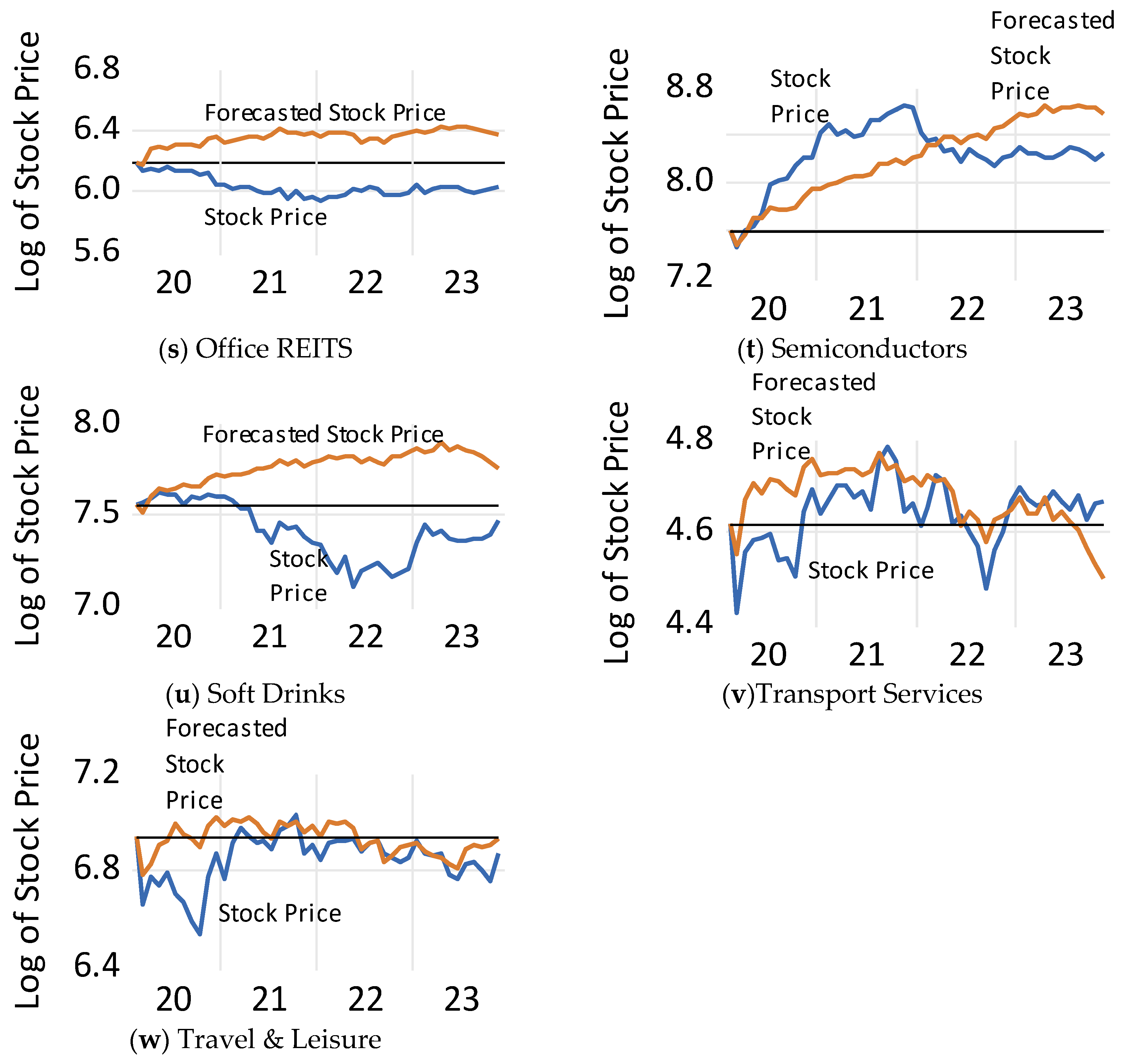
Figure 1 shows actual sectoral returns and predicted sectoral returns during the megacrisis period that began with the pandemic.

Table 2. The root mean squared error of forecasted stock prices using macroeconomic variables and autoregressive integrated moving average (ARIMA) model.

(1)	(2)	(3)	(4)
Sector	Macroeconomic Model	ARIMA Model	Diebold–Mariano Test
	Root Mean Squared Error	Root Mean Squared Error	Squared ErrorTest Statistics
Airlines	0.313	0.338	−14.11 ***
Aluminum	0.396	0.346	4.83 ***
Automobiles	0.168	0.178	−11.47 ***
Banks	0.121	0.199	23.51 ***
Brewers	0.404	0.494	−6.89 ***
Casinos & Gambling	0.130	0.164	−8.00 ***
Cement	0.302	0.335	0.57
Chemicals	0.366	0.390	6.36 ***
Construction	0.217	0.107	−0.46
Consumer Discretionary	0.134	0.244	−6.75 ***
Electrical & Electronic Equipment	0.404	0.442	−0.93
Financials	0.115	00.073	1.88 *
Food Producers	0.197	0.271	−5.23 ***
Fruits & Grains	0.261	0.344	−5.90 ***
Healthcare	0.719	0.781	−5.03 ***
Ind. Transport	0.081	0.115	−4.25 ***
Marine Transport	0.116	0.133	−4.15 ***
Medical Supplies	1.199	1.256	−3.12 ***
Office REITS	0.344	0.381	0.91
Semiconductors	0.319	0.371	−1.29
Soft Drinks	0.419	0.461	−6.61 ***
Transport Services	0.082	0.172	4.23 ***
Travel & Leisure	0.126	0.178	−7.34 ***

Notes: Column (2) reports the root mean squared error for forecasts of stock prices for the sectors listed in column (1) over the March 2020 to November 2023 period using a macroeconomic model estimated over the February 2001 to February 2020 period. The model forecasts sectoral stock returns using: (1) the return on the Malaysian stock market, (2) the return on the world stock market, (3) news about Malaysian consumer price index inflation, (4) the change in the log of the ringgit/dollar exchange rate, (5) the change in the log of the dollar spot price for Dubai crude oil, and (6) the first principal component of 17 Malaysian macroeconomic series. The forecasts over the March 2020 to November 2023 period are obtained using actual out-of-sample values of the macroeconomic variables. Column (3) reports the root mean squared error forecasts of stock prices listed in column (1) over the March 2020 to November 2023 period using autoregressive integrated moving average (ARIMA) models estimated over the February 2001 to February 2020 period. The ARIMA models are selected based on the Akaike Information Criterion, with a maximum possible of four autoregressive coefficients, four moving average coefficients, and one difference in the log of stock prices. Column (4) presents the test statistic for the Diebold–Mariano test calculated using the squared difference between actual and forecasted values. Negative and statistically significant values indicate that the null hypothesis that the models in column (2) and (3) have the same accuracy can be rejected in favor of the model in column (2). Positive and statistically significant values indicate that the null hypothesis that the models in column (2) and (3) have the same accuracy can be rejected in favor of the model in column (3). *** (*) denote significance at the 1% (10%) levels.

compares the root mean squared error (RMSE) from forecasts obtained using the macroeconomic variables with forecasts obtained using autoregressive integrated moving average (ARIMA) models. In all but three cases, the RMSE in column (2) for the model forecasted using macroeconomic variables is lower than the RMSE in column (3) for the model forecasted using ARIMA methods. This indicates that the model used to forecast in Figure 1 outperforms the benchmark ARIMA forecasts in the vast majority of cases. Results of Diebold–Mariano tests in column (4) indicate that in 13 cases, the test statistics are negative and significant, implying that the macroeconomic model provides more accurate forecasts than the ARIMA model. In only four cases, the test statistics are positive and significant, implying that the ARIMA model provides more accurate forecasts than the macroeconomic model.

Figure 2 shows that, in any case, the forecasts using the ARIMA model are very similar to the forecasts using the macroeconomic model. The figure plots the forecasted change in sectoral stock prices in November 2023 using models estimated up until February 2020 and then forecasted using actual out-of-sample values of the right-hand side variables. Regressing the forecasted change using the macroeconomic model on the forecasted change using the ARIMA model yields a coefficient of 1.10 and a t-statistic of 16.0. There is, thus, a close relationship between forecasts using the macroeconomic model and forecasts using the ARIMA model.

The sectors in Figure 1 can be categorized into those that: (1) initially gained when COVID-19 appeared and then fell, (2) those that initially gained and then kept gaining, (3) those that initially lost and then recovered, and (4) those that initially lost and continued losing.

The first category includes medical supplies, healthcare, and semiconductors. Medical supplies stocks in panel (r) more than doubled in value between February and July 2020. Malaysia is a leading supplier of medical supplies (e.g., rubber gloves) and demand for these soared during the pandemic. Medical supply stocks then tumbled and fell logarithmically to more than 100% below their forecasted values by November 2023. Healthcare stocks in panel (o) closely mirrored the performance of medical supply stocks. Semiconductor stocks in panel (t) fell in March 2020 but then gained more than 100% as demand for information and communication technology devices by people working from home drove demand for semiconductors. Between November 2021 and November 2023, however, semiconductor stocks fell 40%. One problem facing the Malaysian semiconductor sector is that it is mired in low-value-added niches of the semiconductor industry, such as assembly and packaging (Wang and Lim 2023).

Aluminum (panel b), after falling briefly in March 2020, grew steadily. Demand for and prices of industrial metals have soared, and Malaysia metal producers have benefited. As aluminum prices have moderated, aluminum stocks are off their highs. Nevertheless, in November 2023 they remained more than 70% above their values in February 2020.

Many sectors initially suffered and then recovered. These include banks (panel d), the financial sector (panel l), and automobiles (panel c). The IMF (2023) reported that Malaysian banks are profitable and the financial system stable. The banking sector’s total capital ratio at the end of 2022 equaled almost 19%, its common equity tier 1 equaled 15%, and its share of nonperforming loans and household debt under repayment assistance both equaled 1.7%. The financial system also has sufficient liquidity. A strong banking sector is important for Malaysian firms, given their dependence on bank credit. The demand for automobiles, after falling as the pandemic arrived, increased as individuals shunned public transportation.

Other sectors suffered initially and then continued to perform badly. These include food producers (panel m), fruits and grains (panel n), brewers (panel e), and soft drink makers (panel u). As people stopped visiting restaurants during the pandemic, these sectors suffered. Then, as the Russia–Ukraine War raised food prices and as inflation forced consumers to economize, these sectors continued to underperform.

Tourism-related sectors, such as airlines (panel a), travel and leisure (panel w), and casinos and gambling (panel f), after suffering when the pandemic arrived, recovered. It is important to note, however, that in November 2023, they remain about 15% below both predicted values and the values they had in February 2020.

The results indicate that several sectors are underperforming three and a half years after the pandemic struck. These include healthcare, medical supplies, semiconductors, food producers, fruits and grains, and tourism-related sectors. The next section considers how to promote economic activity in these sectors that have been hit by economic shocks and often suffered through no fault of their own.

4. Policy Implications

The results in the previous section indicate that both the healthcare and tourism sectors are struggling. One way to stimulate both sectors would be to promote medical tourism. As Kawai and Lee (2015) noted, healthcare in Asian countries can be much cheaper than in other countries and, thus, can attract tourists. SERC (2022) observed that medical tourism in Malaysia offers opportunities for an array of firms, including hotel operators, travel agents, ferry companies, wellness providers, and tourism companies.

ACCCIM (2022), surveying stakeholders, identified several obstacles to firms involved in medical tourism. One is a lack of coordination between ministries responsible for healthcare and tourism. A second is onerous procedures for renewing medical visas, requiring patients to resubmit visa applications every 30 days. A third is inadequate government promotion of medical tourism abroad. A fourth is insufficient knowledge and financial resources among SMEs in this sector. To realize the potential in medical tourism, the government should address these issues.

The Malaysian Rubber Board can increase the demand for medical and household rubber gloves by researching and spreading knowledge about manufacturing biodegradable gloves. The lion’s share of rubber gloves is thrown away. Biodegradable gloves would be desired by environmentally conscious consumers and businesses throughout the world.

The results in the previous section indicate that semiconductor stocks have fallen since November 2021. Wang and Lim (2023) noted that the Malaysian semiconductor industry is mired in low-value-added labor-intensive activities, such as assembly and packaging. Interviewing key observers, they found that the lack of a robust engineering ecosystem prevented Malaysian semiconductor firms from advancing into more complex tasks. They reported that there was insufficient FDI and that technical collaboration between Malaysian semiconductor firms, such as Silterra, and Taiwanese firms, such as ProMos Technologies, did not generate knowledge transfers to Malaysian firms. Hill et al. (2012) observed that Malaysia’s affirmative action programs favoring indigenous Malaysians (bumiputera) over ethnic Chinese and Indian Malaysians deterred foreign investors. Wang and Lim also noted that insufficient spending on research and development (R&D) disadvantaged the Malaysian semiconductor industry.

Experience in economies such as Taiwan indicates that a robust semiconductor industry provides abundant opportunities for firms to participate in the value chain. Malaysia should seek to strengthen this sector. It should train more engineers. It should also seek to attract FDI. One key step would be to ease the affirmative action policies that have prevented the best candidates from becoming CEOs, the most qualified firms from receiving grants, and the most promising students from obtaining scholarships (Rasiah 2010, 2017). Another step would be to recruit workers endowed with tacit knowledge from abroad. For instance, Lim and Pek (2023) have suggested that Malaysia recruit Japanese retirees to promote human capital development in Malaysia. A third would be to boost spending on R&D. As MNCs are seeking to relocate away from China and as the U.S. and Japan are seeking to friendshore their supply chains, creating an attractive environment for foreign investors would help Malaysia to seize the opportunity and grow its semiconductor sector.

SERC (2022) has offered several suggestions for promoting R&D in Malaysia. It noted that, while private companies undertake the lion’s share of R&D in advanced economies, in Malaysia, the private sector accounts for only 43.9% of R&D expenditures. It observed that innovation depends on the government’s funding of science and research. Malaysia should imitate the example of Taiwan, where government research institutes, science parks, private firms, and universities work together in close proximity to help disperse technical knowledge across the economy.

The results in Section 3 indicate that the fruits and grains sector is underperforming. SERC (2022) noted that Malaysia has favorable climate and soil conditions for tropical fruits, including pineapples, bananas, guavas, mangoes, papayas, coconuts, durians, watermelons, and coconuts. ACCCIM (2022) reported that that the food and farming sector is dependent on costly inputs. It argued that both the private sector and the government should promote learning and technology assimilation to reduce this dependence. It also noted that only 5.5% of planted areas produce fruits and vegetables. It observed that the government could increase the land used for fruit and vegetable farming by providing 30-year leases to new farmers if they agree to farm the land for a certain period of time. It also advocated providing leases of 30 years or longer to existing farmers to encourage modernization and re-investment.

The findings in the previous section indicate that food producers have been hit hard over the last three years. SERC (2022) reported that there are 1.9 billion Muslims in the world, and that Malaysia is well-positioned to export halal foods and products to them. Halal certification reassures consumers that the goods have been produced according to Shariah law.

SERC (2022) recommended several steps that Malaysia could take to promote the halal industry. Firstly, the Department of Islamic Development Malaysia (JAKIM) lacks manpower and can, thus, be slow to provide halal certification and can provide poor monitoring and enforcement. Delays in certification hinder businesses from being competitive and poor monitoring and enforcement open the door for businesses to provide fake certification. Fake products can, in turn, tarnish the reputation of the entire Malaysian halal sector. SERC observed that some find the JAKIM guidelines confusing and have to pay extra to navigate the procedures. Other businesses do not apply for halal certification because they believe that the process is too complicated and time-consuming. To help Malaysian entrepreneurs to take advantage of the opportunities of producing halal food, JAKIM should remedy these issues. JAKIM should also work with halal certification agencies abroad to harmonize standards and streamline trade.

5. Conclusions

Many researchers have expressed concern for how contractionary monetary policy in the U.S. will impact emerging market economies (see, e.g., World Bank 2023). Results presented here indicate that, for much of the Malaysian economy, U.S. monetary policy is a non-event. Two different measures of U.S. monetary policy are uncorrelated with Malaysian aggregate stock returns. Banks, rather than being harmed by contractionary U.S. monetary policy as open economy versions of the Bernanke–Gertler model predict, actually benefit from contractionary U.S. monetary policy. Higher interest rates in the U.S. can lead to higher interest rates in Malaysia and benefit banks by increasing the spread between the interest rate they earn on assets and the interest rate they pay on deposits. Contractionary U.S. monetary policy is associated with lower returns on cement and construction stocks. This is consistent with Cho and Rhee’s (2014) finding that contractionary U.S. monetary policy causes a fall in real estate prices in Asia. For most other sectors, however, there is little evidence that U.S. monetary policy matters.

Arteta et al. (2022) found that contractionary U.S. monetary policy shocks lowered equity prices in emerging economies. The results here indicate that U.S. monetary policy matters little for the Malaysian stock market. Future research should investigate why Malaysia is insulated from U.S. monetary policy shocks and whether there are lessons that other emerging market economies can learn from Malaysia’s resilience.

Higher global oil prices increase Malaysian stock returns. Decomposing oil prices into those parts reflecting aggregate demand and oil supply shocks, the results indicate that oil price increases driven by global demand are especially important for Malaysian aggregate stock returns. The evidence also indicates that residual oil price increases, controlling for demand factors, raise stock returns. This reflects the fact that Malaysia, as an oil exporter, benefits from higher oil prices. Future research should extend this approach to investigate how recent oil price shocks are affecting other emerging market economies.

The COVID-19 pandemic buffeted the Malaysian economy, contributing to a fall in real GDP of 5.6% in 2020. Malaysia then vaccinated 95% of its adult population by the end of 2021 and opened its border in 2022. While the Malaysian economy recovered in 2022, the IMF (2022) noted that the recovery has been uneven. The Russia–Ukraine War, beginning in February 2022, also unleashed a rise in prices for oil, food, and other items that affected Malaysia. Droughts, floods, and wildfires related to climate change exacerbated these challenges. Scholars and policymakers have labeled the period after the pandemic began as an era of megacrises (see, e.g., Ramos-Horta et al. 2022).

By comparing sectoral stock market performance since the pandemic began with performance forecasted based on macroeconomic variables, this paper reports that healthcare, medical supplies, food producers, fruits and grains, and tourism-related sectors are underperforming. Some of these industries suffered from recent economic shocks through no fault of their own. This paper offers several recommendations to stimulate these struggling sectors. Future research should investigate whether these sectors in other countries are also underperforming after the pandemic. If not, then it would be instructive to know why these sectors are performing better in other countries than they are in Malaysia.

References

ACCCIM. 2022. Malaysia’s Business and Economic Conditions Survey Report, 1H 2022 and 2H 2022. Kuala Lumpur: Associated Chinese Chambers of Commerce and Industry of Malaysia. [Google Scholar]
Arteta, Carlos, Steven Kamin, and Franz Ruch. 2022. How Do Rising U.S. Interest Rates Affect Emerging and Developing Economies? It Depends. World Bank Policy Research Working Paper 10258. Washington, DC: World Bank. [Google Scholar]
Azis, Iwan, and Willem Thorbecke. 2004. The Effects of Exchange Rate and Interest Rate Shocks on Bank Lending in Indonesia. Economics and Finance in Indonesia 52: 279–95. [Google Scholar]
Bauer, Michael, and Eric Swanson. 2022. A Reassessment of Monetary Policy Surprises and High-frequency Identification. In NBER Macroeconomics Annual 2022. Edited by Martin Eichenbaum, Erik Hurst and Valerie A. Ramey. Chicago: University of Chicago Press, vol. 37. [Google Scholar]
Bernanke, Ben. 2016. The Relationship between Stocks and Oil Prices. Ben Bernanke’s Blog, February 19. [Google Scholar]
Bernanke, Ben, Mark Gertler, and Simon Gilchrist. 1996. The Financial Accelerator and the Flight to Quality. Review of Economics and Statistics 78: 1–15. [Google Scholar] [CrossRef]
Black, Fischer. 1987. Business Cycles and Equilibrium. Hoboken: Wiley. [Google Scholar]
Blanchard, Olivier, Jonathan Ostry, Atish Ghosh, and Marcos Chamon. 2017. Are Capital Inflows Expansionary or Contractionary? Theory, Policy Implications, and Some Evidence. IMF Economic Review 65: 563–85. [Google Scholar] [CrossRef]
Bu, Chunya, John Rogers, and Wenbin Wu. 2021. A Unified Measure of Fed Monetary Policy Shocks. Journal of Monetary Economics 118: 331–49. [Google Scholar] [CrossRef]
Carrière-Swallow, Yan, Pragyan Deb, Davide Furceri, Daniel D. Jiménez, and Jonathan Ostry. 2023. Shipping Costs and Inflation. Journal of International Money and Finance 130: 102771. [Google Scholar] [CrossRef] [PubMed]
Chen, Jiaqian, Tommaso Mancini-Griffoli, and Ratna Sahay. 2014. Spillovers from United States Monetary Policy on Emerging Markets: Different This Time? IMF Working Paper WP/14/240. Washington, DC: International Monetary Fund. [Google Scholar]
Chen, Nai-Fu, Richard Roll, and Stephen Ross. 1986. Economic Forces and the Stock Market. The Journal of Business 59: 383–403. [Google Scholar] [CrossRef]
Cho, Dongchul, and Changyong Rhee. 2014. Effects of Quantitative Easing on Asia: Capital Flows and Financial Markets. The Singapore Economic Review 59: 1–23. [Google Scholar] [CrossRef]
Cox, John, Jonathan Ingersoll, and Stephen Ross. 1985. An Intertemporal General Equilibrium Model of Asset Prices. Econometrica 53: 363–84. [Google Scholar] [CrossRef]
Estrada, Gemma, Donghyun Park, and Arief Ramayandi. 2015. Taper Tantrum and Emerging Equity Market Slumps. ADB Economics Working Paper No. 451. Manila: Asian Development Bank. [Google Scholar]
Fama, Eugene, and James MacBeth. 1973. Risk, Return, and Equilibrium: Empirical Tests. Journal of Political Economy 81: 607–36. [Google Scholar] [CrossRef]
Frankel, Jeffrey, and Gikas Hardouvelis. 1985. Commodity Prices, Money Surprises and Fed Credibility. Journal of Money, Credit and Banking 17: 425–38. [Google Scholar] [CrossRef]
Golub, Stephen. 1983. Oil Prices and Exchange Rates. The Economic Journal 93: 576–93. [Google Scholar] [CrossRef]
Hamilton, James. 2014. Oil Prices as an Indicator of Global Economic Conditions. Econbrowser Weblog, December 14. [Google Scholar]
Hill, Hal, Tham Yean, and Ragayah Zin. 2012. Malaysia: A Success Story Stuck in the Middle? The World Economy 35: 1687–711. [Google Scholar] [CrossRef]
IMF. 2014. World Economic Outlook. Legacies, Clouds, Uncertainties. Washington, DC: International Monetary Fund. [Google Scholar]
IMF. 2022. Malaysia: Staff Report for the 2022 Article IV Consultation. Washington, DC: International Monetary Fund. [Google Scholar]
IMF. 2023. Malaysia: Staff Report for the 2023 Article IV Consultation. Washington, DC: International Monetary Fund. [Google Scholar]
Kawai, Masahiro, and Jong-Wha Lee. 2015. Rebalancing for Sustainable Growth: Asia’s Postcrisis Challenge. Tokyo: Springer. [Google Scholar]
Kilian, Lutz. 2009. Not All Oil Price Shocks Are Alike: Disentangling Demand and Supply Shocks in the Crude Oil Market. American Economic Review 99: 1053–69. [Google Scholar] [CrossRef]
Krugman, Paul. 2001. Analytical Afterthoughts on the Asian Crisis. In Economic Theory, Dynamics and Markets. Research Monographs in Japan-U.S. Business & Economics. Edited by Takashi Negishi, Rama Ramachandran and Kazuo Mino. Boston: Springer, vol. 5. [Google Scholar]
Lim, Guanie, and Aaron Pek. 2023. Japanese Retirees Can Boost Malaysia’s Industrial Advance. Nikkei Asia, July 19. [Google Scholar]
Liu, Jing, Doron Nissim, and Jacob Thomas. 2007. Is Cash Flow King in Valuations? Financial Analysts Journal 63: 1–13. [Google Scholar] [CrossRef]
McMillan, David. 2021. Predicting GDP Growth with Stock and Bond Markets: Do They Contain Different Information? International Journal of Finance and Economics 26: 3651–75. [Google Scholar] [CrossRef]
Petralia, Kathryn, Thomas Philippon, Tara Rice, and Nicholas Véron. 2019. Banking Disrupted? Financial Intermediation in an Era of Transformational Technology. Geneva: International Center for Monetary and Banking Studies. [Google Scholar]
Ramos-Horta, José, Danilo Türk, Laura Chinchilla Miranda, and Han Seung-Soo. 2022. Managing the Megacrisis of 2022. Project Syndicate Weblog, July 19. [Google Scholar]
Rasiah, Rajah. 2010. Catch Up in Integrated Circuits Production: Malaysia Compared to Korea and Taiwan. In Inaugural Public Lecture of the Malaysian Centre of Regulatory Studies. Kuala Lumpur: University of Malaya, October 13. [Google Scholar]
Rasiah, Rajah. 2017. The Industrial Policy Experience of the Electronics Industry in Malaysia. In The Practice of Industrial Policy: Government-Business Coordination in Africa and East Asia. Edited by John Page and Finn Tarp. Oxford: Oxford University Press. [Google Scholar]
Ready, Robert. 2018. Oil Prices and the Stock Market. Review of Finance 22: 155–76. [Google Scholar] [CrossRef]
Ross, Stephen. 2001. Finance. In The New Palgrave Dictionary of Money and Finance. Edited by Peter Newman, Murray Milgate and John Eatwell. London: Macmillan Press. [Google Scholar]
SERC. 2022. Exporting for Growth: The SME’s Perspective. Kuala Lumpur: Socio-Economic Research Centre. [Google Scholar]
Thorbecke, Willem. 2016. Investigating the Effect of U.S. Monetary Policy Normalization on the ASEAN-4 Economies. RIETI Discussion Paper 16-E-070. Tokyo: Research Institute of Economy, Trade and Industry. [Google Scholar]
Thorbecke, Willem. 2019. How Oil Prices Affect East and Southeast Asian Economies: Evidence from Financial Markets and Implications for Energy Security. Energy Policy 128: 628–38. [Google Scholar] [CrossRef]
Velinov, Anton, and Wenjuan Chen. 2015. Do Stock Prices Reflect their Fundamentals? New Evidence in the Aftermath of the Financial Crisis. Journal of Economics and Business 80: 1–20. [Google Scholar] [CrossRef]
Wang, Hongchuan, and Guanie Lim. 2023. Catching-Up in the Semiconductor Industry: Comparing the Chinese and Malaysian Experience. Asian Journal of Technology Innovation 31: 49–71. [Google Scholar] [CrossRef]
World Bank. 2023. East Asia and the Pacific Economic Update, April 2023: Reviving Growth. Washington, DC: World Bank. [Google Scholar]
Figure 1.
Actual and predicted Malaysian stock prices since the COVID-19 pandemic began. Notes: The blue line represents actual sectoral stock prices, the orange line represents forecasted sectoral stock prices, and the black horizontal line represents the value of sectoral stock prices in February 2020. Forecasted stock prices are obtained from a regression of the sectoral stock returns on (1) the return on the Malaysian stock market, (2) the return on the world stock market, (3) news about Malaysian consumer price index inflation, (4) the change in the log of the ringgit/dollar exchange rate, (5) the change in the log of the dollar spot price for Dubai crude oil, and (6) the first principal component of 17 Malaysian macroeconomic series. The regressions are run over February 2001 to February 2020 period. Actual out-of-sample values of the right-hand side variables are then used to forecast stock prices (the orange line) over the March 2020 to November 2023 period.
Figure 2.
Forecasted changes in sectoral stock returns using macroeconomic variables and using an autoregressive integrated moving average model. Notes: The horizontal axis presents forecasted changes in sectoral stock returns over the February 2020–November 2023 period using macroeconomic variables. The vertical axis presents forecasted changes in sectoral stock returns over the February 2020–November 2023 period using autoregressive integrated moving average (ARIMA) models. For the forecasts using the macroeconomic models, sectoral returns over the February 2001 to February 2020 period are regressed on: (1) the return on the Malaysian stock market, (2) the return on the world stock market, (3) news about Malaysian consumer price index inflation, (4) the change in the log of the ringgit/dollar exchange rate, (5) the change in the log of the dollar spot price for Dubai crude oil, and (6) the first principal component of 17 Malaysian macroeconomic series. Actual out-of-sample values of the macroeconomic variables are then used to obtain forecasts of stock prices in November 2023. For the forecasts using the ARIMA models, the specification for each sector is selected based on the Akaike Information Criterion, with a maximum possible of four autoregressive coefficients, four moving average coefficients, and one difference in the log of stock prices. The ARIMA model is estimated over the February 2001 to February 2020 period. Actual out-of-sample values of the right-hand side variables are then used to obtain forecasts of stock prices in November 2023.