4.1. Descriptive Statistics
Table 1 presents the descriptive statistics of the logarithmically transformed indices of European financial markets, European carbon emission trading system (EU-ETS) indices, and the CBOE oil price volatility index (CBOE). As illustrated in
Table 1, the financial markets of Finland and Denmark demonstrate elevated average stock indices, with values of 7.18 and 7.47, respectively. This stands in contrast to their counterparts in other European economies and the broader Eurozone. In contrast, Italy’s stock market records the lowest average equity market indices over the past decade, with a value of 5.23 compared to other European economies.
Contemplating a shift away from the Italian stock market could be a prudent move to mitigate potential risks associated with its comparatively lower average equity market indices. This is primarily because the Italian financial market also exhibited a higher standard deviation value of 0.1411 when contrasted with the majority of European economies’ stock markets, including those of Belgium, Finland, and Germany, as well as the standard deviation value of the entire Eurozone. However, among the economies of Europe, Denmark and the Netherlands showed greater variances from the mean in both directions (upwards and downward), which may be attributable to their largest standard deviations (SD) of 0.30 and 0.28, respectively. As a result, European investors with a higher risk tolerance might discern opportunities in Denmark and the Netherlands, considering their potential for greater returns (upside variation). It is crucial to acknowledge, however, that this potential comes with the trade-off of heightened risk (downside variation).
Remarkably, the standard deviation values of 1.05 for the EU-ETS and 0.37 for OVZ exceed the observed standard deviation value across all European financial markets. Elevated volatility in carbon markets might indicate susceptibility to shifts in environmental policies or regulations. It is imperative for investors to diligently observe and evaluate the potential repercussions of regulatory changes in these markets. The heightened volatility in the oil price volatility index implies heightened risk in the energy sector. Investors holding oil-related assets should prudently oversee and manage their portfolios, considering the potential consequences of fluctuations in oil prices. This, in turn, underscores our motivation to scrutinize the influence of EU-ETS and OVZ on European financial markets. Moreover, only the financial markets of Belgium and Finland, as well as the CBOE oil price volatility index, showed excess kurtosis. This may indicate the presence of extreme values and outliers due to the leptokurtic distribution of the data.
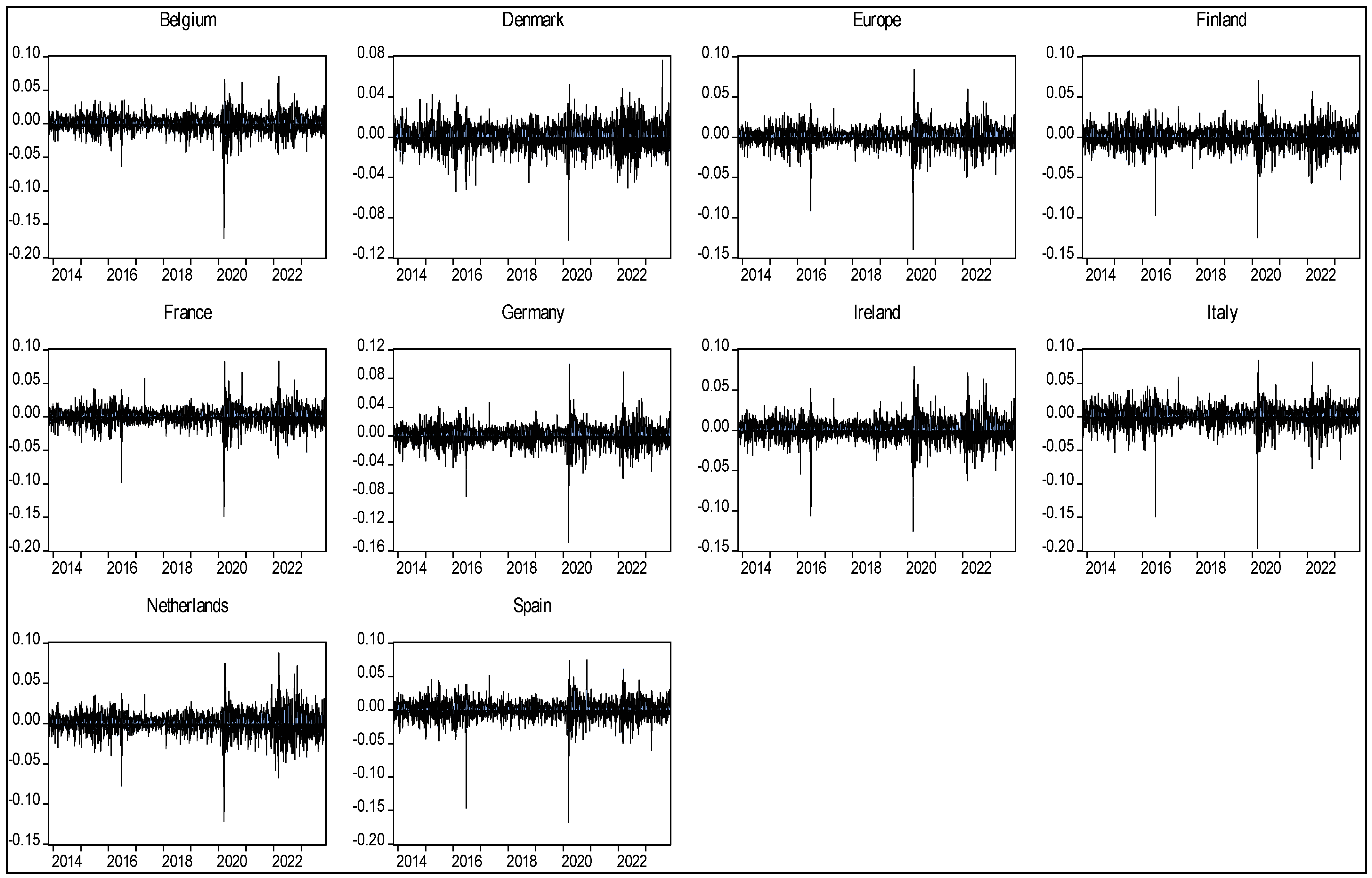
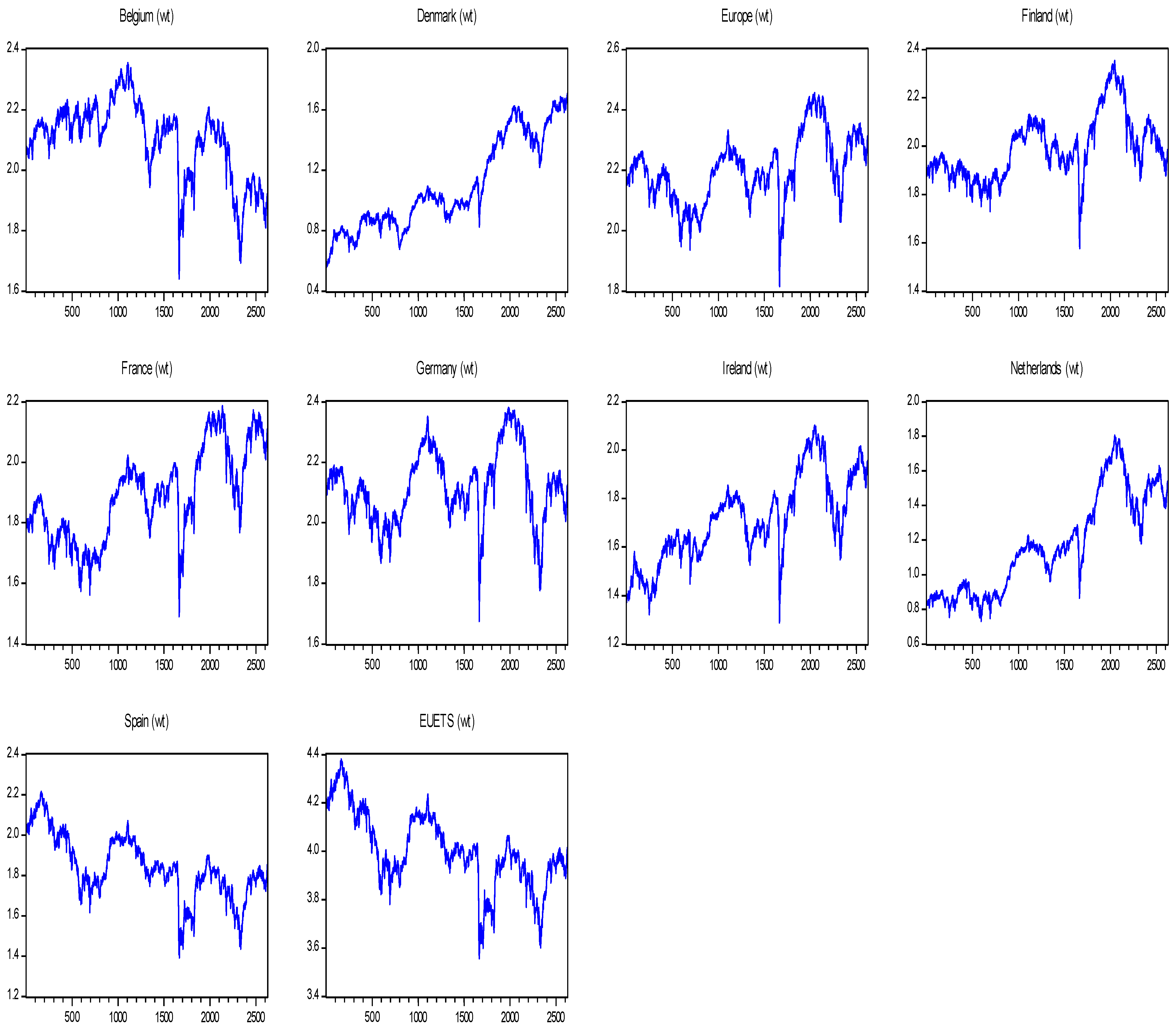
Figure 1 visually illustrates the returns of equity markets across European economies, while
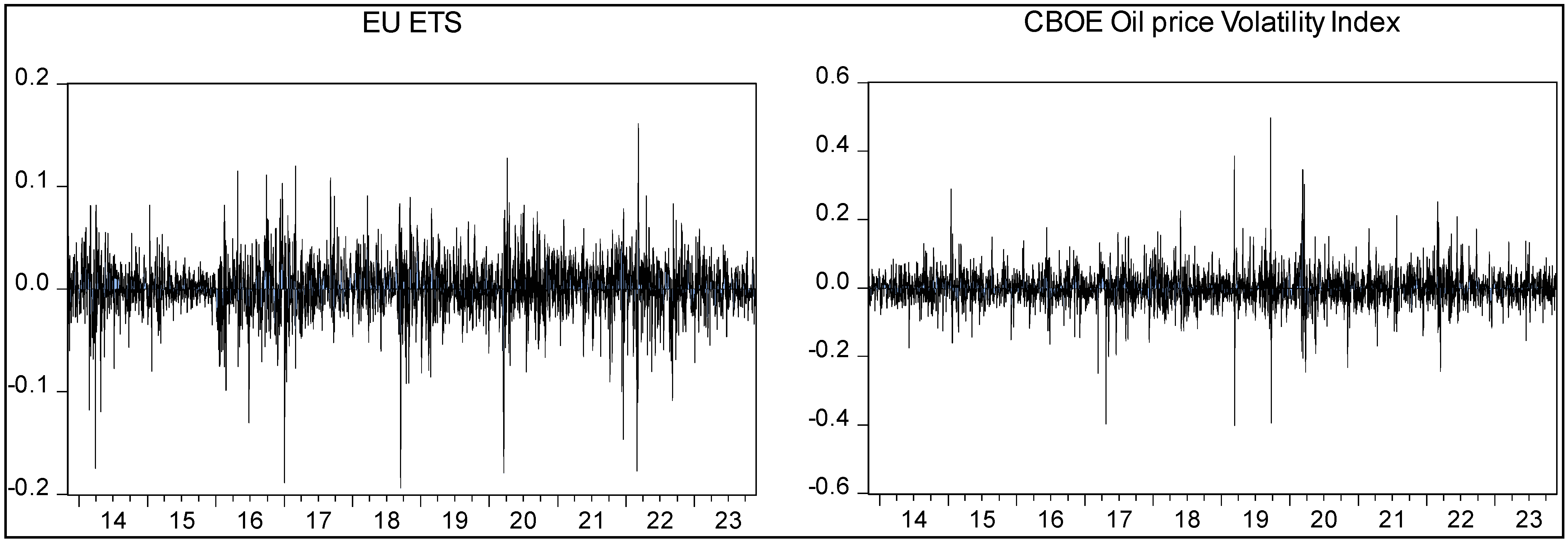
Figure 2 displays the returns in the European carbon emission trading market (EU-ETS) and the fluctuations in the CBOE oil price volatility index. In
Figure 1 it is evident that all European financial markets encountered heightened upside and downside fluctuations between 2014 and 2016, during the COVID-19 era (from 2020 to the end of 2021), and after 2021. A significant factor contributing to these variations in European financial market returns from 2014 to 2016 was the severe economic challenges faced by Greece, leading to a debt crisis. In 2016, the UK conducted a referendum on its European membership, and the majority voted in favor of leaving (Brexit), causing widespread economic and political repercussions. Furthermore, the COVID-19 pandemic significantly affected the world economy and has caused extreme supply chain disruptions.
Both
Figure 1 and
Figure 2 depict increased upside and downside fluctuations in European equity market returns, as well as in OVZ and EU-ETS returns, respectively, in the post-COVID-19 era (after 2021). A key contributing factor to these fluctuations is the impact of energy price variations, including those of oil and natural gas, on European economies, EU-ETS, and the oil price volatility index (
Bourghelle et al. 2021). Moreover, uncertainties in the global economic conditions post COVID-19 can also contribute to the fluctuations observed in EU-ETS (
Li et al. 2022) and equity returns (
Yang et al. 2021). This motivates researchers to further explore the impact of EU-ETS on the European financial system, incorporating the oil price volatility index (OVZ) as a control measure.
Table 1 also indicates that indices of the European carbon emission trading market and European financial markets are integrated in the same order. Specificallys, at this level, both the EU-ETS and European financial market indices display non-stationary characteristics. However, when the initial difference is taken, the mean and variance of both variables remain constant, indicating (
I(1)) dynamics. Nonetheless, the CBOE volatility index for oil prices is stationary at level, i.e., (
I(0)).
In light of the aforementioned information, when dealing with variables exhibiting different orders of integration, the autoregressive distributive lag model (ARDL) approach emerges as a more practical and resilient method (
Suleman et al. 2022). The stationary characteristics of returns in the EU-ETS and European financial markets are evident from
Figure 1 and
Figure 2, respectively. Notably, in the literature,
Mirza and Kanwal (
2017) have also incorporated the
Johansen and Juselius (
1990) test for co-integration before employing the ARDL approach by
Pesaran et al. (
2001).
Table 2 illustrates the results of the co-integration analysis using the
Johansen and Juselius (
1990) method, aiming to identify long-run co-integrating relationships between EU-ETS returns and financial market returns for Belgium, Finland, France, Germany, Ireland, Italy, Netherlands, Spain, Denmark, and the entire Eurozone. The findings in
Table 2 indicate the presence of long-term co-integration between the variables, justifying the use of the ARDL approach to explore both the short- and long-term impacts of EU-ETS returns on the financial market returns of respective EU economies.
4.2. ARDL Approach and Practical Implications for Long-Term Shareholders and Short-Term Speculators
Table 3 displays the estimates derived from the ARDL approach proposed by
Pesaran et al. (
2001). These estimates aim to assess the short- and long-term reactions of European financial market returns to the fluctuations in both the European carbon emission trading market (EU-ETS) returns and the CBOE oil price volatility index (OVZ). Additionally, as part of residual diagnostics, we provide the results of the Breusch–Pagan heteroscedasticity test (
Breusch and Pagan 1979), the Durbin–Watson (DW) test for autocorrelation (
Durbin and Watson 1951), and the RESET test for model misspecification, ensuring the correct functional form of variables
Ramsey (
1969).
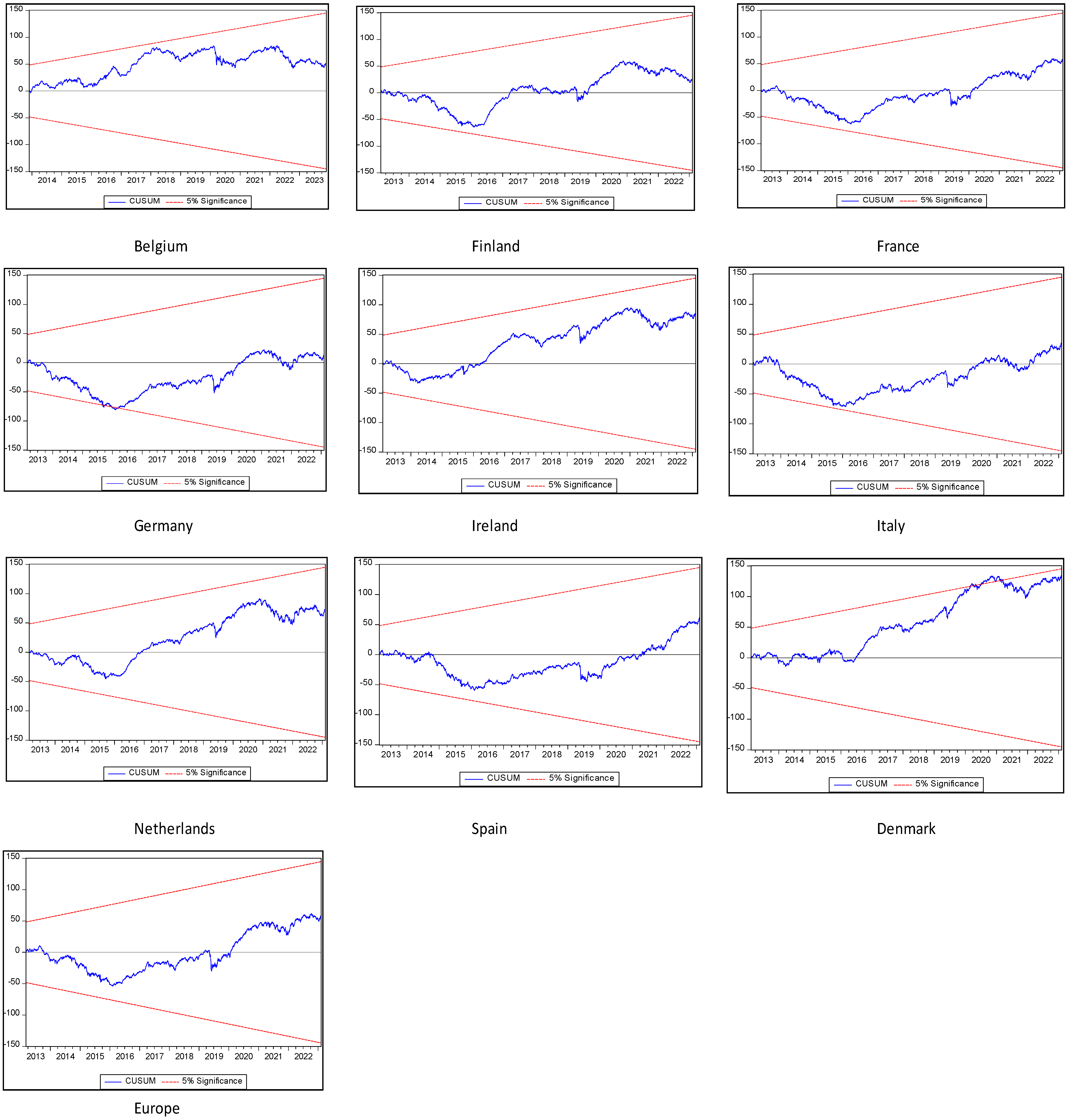
Moreover,
Figure 3 presents a graphical representation of the Cumulative Sum Test (CUSUM) test for ARDL model stability.
Table 3 shows that long-term co-integration is established between European carbon emission trading market (EU-ETS) returns, the CBOE oil price volatility index, and financial market returns of Belgium, France, Germany, Spain, and the whole of Europe. This is generally due to the higher K-statistics values compared to the lower and upper bound critical values and negative and statistically significant values of error correction terms (ECTs). Error correction terms determine whether a model is correcting its long-term disequilibrium at a particular speed of adjustment and signify a long-term co-integrating association between the variables. According to
Table 3, EU-ETS has an adverse long-term effect of 10.22% and 10.13% on the financial market returns of Belgium and Spain, whereas EU-ETS has a significant positive long-run effect of 9% and 3.98% on the financial market returns of France and the whole of the Eurozone. However, in the case of Finland, Ireland, Italy, the Netherlands, and Denmark, long-term co-integration cannot be established. In contrast to the effect of EU-ETS on European financial market returns, the CBOE oil price volatility index has a consistent long-term adverse effect of 19.2%, 22.18%, 27.13%, and 19.41% on the financial market returns of France, Germany, Spain, and the Eurozone. These results diverge from prior research, as earlier studies primarily center on examining the impact of the Chinese carbon emission trading system on the financial performance of Chinese sectors (
Zhang and Han 2022;
Yu et al. 2022;
Chen et al. 2023;
Yin et al. 2019). However,
Sun et al. (
2022) reported a weak association between Chinese carbon trading market returns and energy-related firms.
One rationale for the negative long-term impact of the EU Emission Trading System (EU-ETS) on the financial market returns of Belgium and Spain lies in the perception that the carbon emission trading mechanism functions as a potent driver for economic development (
Bibi et al. 2021). In the context of Belgium and Spain, the stock markets reflect the status of economic development. Additionally, increased economic activity and positive equity market performance may lead to a surge in energy demand, potentially elevating carbon emissions (
Sousa et al. 2014). This, in turn, could drive up prices in the carbon emission trading market (
Jiménez-Rodríguez 2019). Consequently, the heightened prices in the carbon emission trading market may exert increased pressure on the financial systems of Belgium and Spain to comply with governmental regulations on emission reduction (
Zheng et al. 2021;
Suleman et al. 2023b). Such compliance pressures could, in the end, result in an adverse impact on carbon trading market returns in European stock markets. Another contributing factor is that prices in the carbon emission trading market have the potential to influence the economic incentives and capital costs of businesses, as elucidated by
Oestreich and Tsiakas (
2015). These effects may subsequently manifest in the pricing dynamics of the stock markets of Belgium and Spain.
In addition to the aforementioned reasons explaining the negative long-term impacts of the EU Emission Trading System (EU-ETS) on financial market returns, it is noteworthy that the financial markets of the Eurozone region and France exhibited a favorable response to increased EU-ETS returns. This positive reaction is primarily attributed to the substantial positive long-term effects of 9% and 3.98% on the financial market returns of France and the entire Eurozone, respectively. One rationale for this positive outcome is that European companies often operate well below their assigned carbon allowances, resulting in excess allowances available for trading. This strategic approach proves particularly advantageous when carbon trading prices are on an upward trend, such as during periods of higher carbon prices (
Wen et al. 2020a;
Zheng et al. 2021). In market environments of this nature, businesses with lower carbon footprints have the opportunity to capitalize on their excess allowances through trading. This not only contributes to an overall decrease in carbon emissions but also improves their financial performance (
Suleman et al. 2023b). Consequently, higher carbon prices result in a favorable impact on the returns of the French stock market. Additionally, the ability of companies relying on green energy to engage in carbon permit trading introduces an additional dimension to their financial benefits. As underscored by
Oestreich and Tsiakas (
2015), the economic advantages derived from trading carbon permits during bullish market phases can be substantial.
Our findings offer several practical implications for long-term shareholders. Firstly, businesses operating within Spain and Belgium may explore long-term sustainable practices aligned with environmental goals while also considering the financial consequences of EU-ETS on their operations. Consequently, incorporating the influence of carbon trading prices on stock returns in these markets is imperative for a comprehensive long-term investment strategy. Measures should be considered to alleviate the negative impact on stock returns without compromising environmental objectives. For instance, Belgian and Spanish companies could implement long-term carbon reduction policies by transitioning their manufacturing and production processes from carbon-intensive resources to green energy resources (
Wen et al. 2020a). Hence, the utilization of green energy resources and the internalization of carbon emission-free mechanical processes may offer a safeguard against the additional pressure arising from escalating carbon prices (
Oestreich and Tsiakas 2015), and it will enhance stock market performance in Spain and Belgium.
Secondly, in the long term, the financial markets in France and the entire Eurozone demonstrated a positive response to the increase in carbon trading prices. As a result, long-term investors from Belgium and Spain may identify investment opportunities in companies operating within France and the Eurozone that align with or benefit from the favorable impact of rising carbon trading prices on financial markets. Shareholders in France might contemplate adjusting their long-term investment plans based on the observed positive response in the equity market to EU-ETS, potentially reallocating resources to regions or industries showing growth linked to carbon trading. Long-term investors in France, Belgium, and Spain should be mindful of how government policies and regulations concerning carbon emissions and trading can influence financial markets. Changes in regulatory frameworks have the potential to impact investment strategies.
Thirdly, in the case of Finland, Ireland, Italy, Netherlands, and Denmark, the long-term co-integration between EU-ETS and the financial markets of these economies cannot be established, and there is no significant EU-ETS effect on the financial markets. Investors should conduct thorough country-specific analyses, recognizing that the dynamics of carbon trading impacts differ across regions. Strategies should be tailored to the unique characteristics of each market. Companies in these regions may allocate resources and efforts toward areas with more significant financial implications rather than prioritizing carbon trading price considerations in their long-term business plans.
Fourthly, the CBOE oil price volatility index also has an adverse effect on the financial market returns of France, Germany, Spain, and aggregated Eurozone equity market returns. In the long run, a 1% increase in OVZ causes the equity market returns of France, Germany, Spain, and the aggregated Eurozone to depreciate by 19.25%, 22.18%, 27.13%, and 19.41%, respectively. Due to the fact that businesses and investors in these economies may be heavily exposed to either the equity or oil market, understanding this negative correlation is crucial for risk control. Hedging strategies can be employed to offset potential losses in one market with gains in the other. Energy companies, especially in France, Germany, and Spain, may experience a long-term inverse relationship between their stock prices and oil prices. Lower oil prices might benefit consumers and oil-independent industries but could negatively affect the profitability of energy-dependent companies (see
Hadhri 2021).
Table 3 also shows that the short-term positive (adverse) impact of the European carbon emission trading market (CBOE oil price volatility index) is more pronounced and consistent for all financial market returns in Belgium, Denmark, Finland, France, Germany, Ireland, Italy, Netherlands, Spain, and the Eurozone. Based on these findings, we also intend to explore a few useful ramifications for short-term traders.
Initially, European corporations can utilize these results to inform short-term strategic choices concerning their environmental practices. Firms witnessing short-term positive stock price responses to returns in the carbon emission trading market may find motivation to embrace eco-friendly policies, given the potential positive impact on their stock performance. Subsequently, this illustrates that a favorable influence on stock prices could prompt governments and regulatory bodies to formulate and enforce more resilient and market-friendly mechanisms for carbon trading. Thirdly, the positive interconnection between markets has the potential to enhance overall market efficiency. The rapid transmission of information and news from one market to another reduces the probability of price disparities and accelerates the speed at which markets incorporate pertinent information. Fourthly, if the EU-ETS market undergoes a positive trend, it could initiate a feedback loop where investors in the equity market respond positively to this trend. Recognizing these behavioral aspects becomes crucial for participants in the market. Lastly, fluctuations in oil prices may hold implications for economic growth, inflation, and consumer spending. Short-term investor sentiment can be influenced by movements in both markets. For instance, a downturn in the equity market might trigger heightened demand for secure assets such as oil, and vice versa. Furthermore, traders and short-term European investors might devise strategies capitalizing on the inverse correlation between equity and oil markets. During periods of equity market downturns, opportunities to profit from potential increases in oil prices may arise.
4.4. Robustness Analysis
We adopted a rigorous approach to re-evaluate co-integration analysis, addressing the potential impact of structural breaks on our findings. Initially, we incorporated dummy variables into the co-integration analysis to account for these structural breaks. This methodology was crucial for capturing and mitigating the effects of any sudden shifts or changes in the underlying data. To further enhance the robustness of our analysis, we integrated the methodological framework proposed by
Franses and Lucas (
1998). This framework is specifically designed to estimate co-integration in the presence of outliers, providing a more comprehensive understanding of the relationships within the data. It can be contended that the methodology resilient to outliers is nearly synonymous with conventional Gaussian-based analysis, incorporating supplementary dummy variables (
Franses and Lucas 1998).
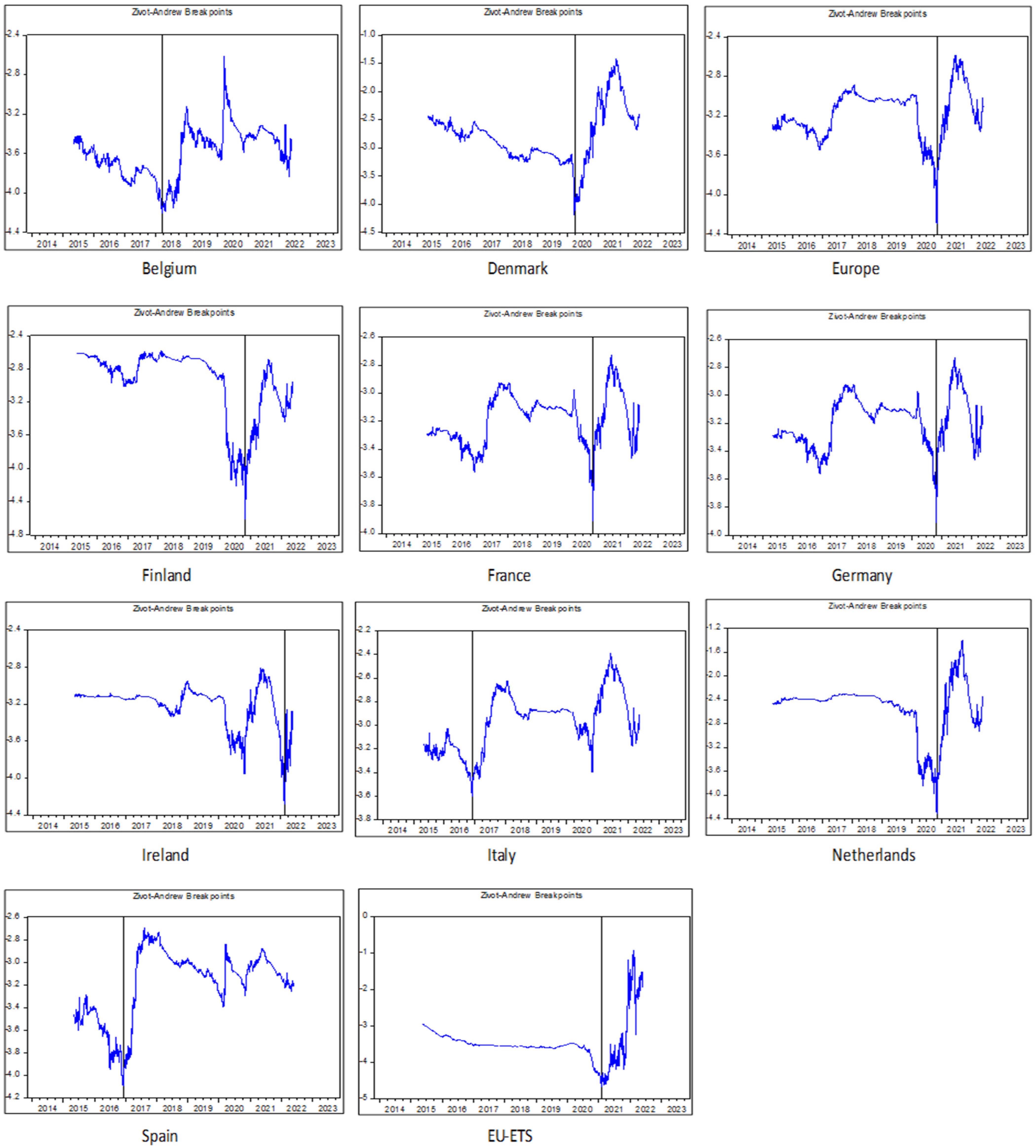
Building on the work of
Johansen and Juselius (
1990), we extended our analysis to include considerations for structural breaks. We employed the
Zivot and Andrews (
1992) unit root test to identify these breaks in the time series data. Once identified, dummy variables were introduced to analyze co-integration in the presence of structural breaks, following the approach outlined by Søren
Johansen et al. (
2000).
Figure 4 visually illustrates the presence of structural breaks in both the carbon emission trading market and European financial markets. Meanwhile,
Table 5a details the specific dates of these structural breaks in the time series data, providing a clear understanding of when significant shifts occurred. With the precise identification of structural break points, we proceeded to re-estimate the
Johansen and Juselius (
1990) test for co-integration. This step was essential to ensure the robustness of our findings and account for any changes in the underlying dynamics of the markets. The results of our analysis are presented in
Table 5b, which explicitly outlines the co-integration analysis in the presence of structural breaks. Notably,
Table 5b demonstrates that long-term co-integration persists even in the presence of structural breaks. This finding is pivotal for understanding the enduring relationships between variables in the European carbon emission trading and financial markets despite the occurrence of significant structural breaks. Overall, our meticulous approach strengthens the reliability and validity of the co-integration analysis in the context of dynamic and changing market conditions.
Conventional tests like co-integration and unit root exhibit sensitivity to anomalous occurrences like anomalies and structural disruptions. To examine the impact of these occurrences, we employ the outlier-robust co-integration approach by (
Franses and Lucas 1998). When traditional co-integration findings may be influenced by a few anomalous observations, our outlier-robust co-integration test offers a novel diagnostic tool for indicating this possibility. The fact that the suggested robust estimator may be used to determine weights for each observation is a key component of our methodology. Therefore, it may be utilized to determine the general dates of atypical occurrences. Additionally,
Bohn Nielsen (
2004) verified the findings of
Franses and Lucas (
1998).
In order to implement the outlier robust co-integration analysis,
Franses and Lucas (
1998) considered the standard vector auto-regression process as follows:
In order to mitigate the impact of outliers,
Lucas (
1997) introduced a Johansen-type testing methodology that relies on non-Gaussian pseudo-likelihoods. The specific instantiation of this approach in the present study is outlined as follows: the parameters in Equation (9) are estimated by employing Student-t pseudo-likelihood with v degrees of freedom.
It is essential to highlight that the vector of unknown parameters is denoted as
. It is crucial to emphasize that the likelihood mentioned in Equation (10) is employed as a pseudo-likelihood, following the conceptual framework introduced by
Gourieroux et al. (
1984). It is important to note that in this approach, the distribution of the error term, denoted as
, is not constrained to be Student-t distributed. Rather, it is only required to satisfy specific weak conditions, as elucidated by
Lucas (
1997). The adoption of the Student-t pseudo-likelihood in Equation (10) serves as a method to address the impact of anomalous data structures on the inference of unit roots. The co-integration test, formulated on the basis of the Student-t pseudo-likelihood, is constructed in the following manner:
Equation (11) relies on a test involving a ratio of two pseudo-likelihoods, which we refer to as a pseudo-likelihood ratio (PLR) test. The weights for the individual observations are obtained as follows:
when the disturbances (represented as
) exhibit independence and identical distribution (iid) characteristics, each having a zero mean and unit variance, the Student-t maximum pseudo-likelihood (MPL) estimator is employed to address this scenario as follows:
In relation to parameter
, let
represent the ultimate estimate. Subsequently,
can be construed as the arithmetic mean of the reweighted sample
.
This derivation stems from the equivalence of the expression of
is the same as
, as readily observed to adhere to condition (13). It is noteworthy that the upper bound of
is not confined to 1 but is rather constrained by (
v + l)/
v. Additionally, parameter
can be construed as the estimator for
u in the weighted regression model through the ordinary least squares (OLS) methodology.
The parameter
may be construed as the weight assigned to the observation at time
i. A diminished value of
signifies that the observation diverges from the overall model pattern. Conversely, an alternative interpretation of
involves considering it as the reciprocal of the standard deviation of the error term. In a manner analogous to the Student-t Maximum Penalized Likelihood (MPL) estimator applied to Equation (12), the Student-t MPL estimator for Equation (9) may be conceptualized as the Gaussian MPL estimator applied to a weighted iteration of Model (1). The assigned weights are determined as follows:
Figure 5 shows the weights of the observations associated with the conventional European financial market and carbon emission trading market indices, whereas
Table 6 shows that co-integration between the carbon emission trading market and conventional financial market returns when utilizing the outlier robust framework of (
Franses and Lucas 1998) to test the co-integration based upon the pseudo-likelihood ratio (PLR) trace test.
Table 6 presents the pseudo-likelihood ratio (PLR) tests designed to evaluate the hypotheses H0: r ≤ 0 against the alternative H1: r = 1. In this context, ‘r’ represents the number of co-integrating relations, ‘p’ signifies the order of the Vector Autoregressive (VAR) model utilized for test computation, and ‘u’ denotes the degrees-of-freedom parameter employed in the usual likelihood method. The symbols *, **, and *** signify significance levels at 10%, 5%, and 1%, respectively. Critical values are obtained from (
Franses and Lucas 1998) under the conditions of drift. The superscripts ‘a’ and ‘b’ correspond to the order of the model associated with the minimum value of the Akaike and Schwarz Information Criteria, respectively.


