A Solvency II Partial Internal Model Considering Reinsurance and Counterparty Default Risk

Abstract

Estimating the expected capital and its variability is a crucial objective for a non-life insurance company, which enables the firm to develop effective management strategies. Many studies have been devoted to this topic, with simulative approaches being especially employed for solving the complexity of the interacting risks, not manageable through closed-form solutions. In this paper, we present a realistic framework based on Solvency II for the definition of next-year capital of a non-life insurer, including reinsurance treaties and counterparty default risk, in a multi-line of business setting. We determine the mean and variance of the stochastic capital considering both quota share and excess-of-loss reinsurance. We show how these closed-form results enable the analysis of many different real-world strategies, granting the insurer the possibility of choosing the optimal policy without the computational resources and time constraints required by simulative approaches.

1. Introduction

The core business of a non-life insurance company is represented by its underwriting activity, consisting in the offering of coverage against risks in exchange for the payment of a premium. In practice, the company receives (in advance) the premiums from the policyholders and pays the claims, in case of occurrence of the covered events. These two items, premiums and claims, are the main elements determining the technical results and, broadly, the future capital of the company. As a part of the management of a firm, the insurer needs to assess the effect of its policies on the amount of premiums and the associated risks that translates into claims. In this way, the insurer can estimate the expected capital and the associated uncertainty, from which it can choose the policy resulting in the optimal result according to its risk/return preferences.

In the actuarial literature, many studies have been devoted to the modelling of the capital of a non-life insurer and more generally to the development of the so-called “risk theory”, with Daykin et al. (1993) providing quite a detailed reference on this argument. The main stochastic variable analysed in this context consists in the aggregate claim amount, which represents the underwriting risk component of the business. In these studies, many closed formulas for the main moments of the stochastic capital of a non-life insurer are developed, typically based on some specific assumptions. In practice, however, the underwriting risk is generally not the single risk for an insurance company. Indeed, in order to balance the uncertain benefits of its activity with the associated risks, insurance companies typically purchase risk-covering instruments like reinsurance treaties. These contracts can be considered an insurance for insurers, since they consist in the transfer of a risk from one party to another through the payment of a premium. Therefore, a more practical and applicable model for real-world scenarios should take into account the possibility of reinsurance treaties.

In the actuarial literature, the stochastic capital of an insurance company considering the presence of reinsurance has been the object of studies typically connected to the topic of optimal reinsurance, where Borch (1960) and Arrow (1963) can be considered seminal papers on this argument. Other results, based on closed formulas connected with optimal reinsurance, have been obtained in Kaluszka (2001), where closed formulas are derived for a quite general structure under mean and variance premium principles, and in Chi and Zhou (2017), in which an optimisation criterion is used based on the minimisation of a general two-dimensional function of the mean and variance of the insurer’s total risk exposure. Optimal risk transfer in presence of multiple reinsurers is instead analysed in Asimit et al. (2013), with closed-form solutions elaborated for some particular settings.

Relatively recently, also pushed by the development of the European framework of Solvency II European Parliament and Council (2009), the actuarial literature shifted its focus towards the analysis of the determination of the required capital for ensuring the solvency of the firm. In this new emerging framework, Clemente et al. (2015) develop a Partial Internal Model based on the Solvency II framework, which extends the classical collective risk model to also include expense as a stochastic variable. Moreover, they also analyse the presence of reinsurance treaties, both quota share (QS) and excess-of-loss (XL) treaties, on the exact moments of the distribution of technical result and investigate the effect of QS commission rates on the variability of distribution. Connected to the problem of optimal non-life reinsurance and the Solvency II framework, Asimit et al. (2015) analyse the optimal policy for an insurer whose objective is the minimisation of its risk exposure. They formulate two optimal reinsurance models, depending on the approach used for calculating the risk margin of reserve risk and prove that a two-layer reinsurance contract is the optimal policy in the defined context. The problem of optimal reinsurance from the insurer’s point of view is also analysed in Cai et al. (2014), in a framework consistent with that of Solvency II, requiring a regulatory initial reserve and also accounting for default risk. Optimal reinsurance strategies are derived for two “opposite” objectives: maximising the expected utility of the insurer’s terminal wealth or minimising the value at risk of the insurer’s total retained risk. Related to the consideration of the default of the reinsurer, Boonen and Jiang (2023) analyse the problem of Pareto-optimal reinsurance in presence of default risk. They show that the optimal indemnity function depends on whether solvency regulation is taken into account or not.

Following the idea of a partial internal model, based on the Solvency II framework, we extend the classic capital modelling of Clemente et al. (2015) also considering the counterparty default risk, connected to the presence of reinsurance companies, as in Cai et al. (2014). Hence, we propose a framework for the analysis of the insurance capital from the existing literature considering a realistic setting with the presence of reinsurance, potentially offered by multiple reinsurers and taking into account counterparty default risk. The model that we define is an extension of Crisafulli (2023) and can potentially be used by a non-life insurer as a partial internal model for premium and default risk, also accounting for reinsurance. We derive the first two moments of the stochastic next-year capital in a closed form and show how these results allow for the efficient frontier of reinsurance strategies to be derived without the computational time and the approximation required by simulative approaches. Finally, while the problem is specific to the actuarial context, it helps to demonstrate the strength of closed-form solutions and their application to optimal selection compared to simulative approaches, when the number of combinations to be analysed is infeasible in terms of computational time and accuracy.

The following sections of this paper are organised as follows. In Section 2, we present the modelling of the capital of a non-life insurance company in a one-year time horizon, describing all its components, with a focus on reinsurance and counterparty risk. In Section 3, we present a first extension of the risk reserve model by adding the possibility of reinsurance and considering the associated counterparty risk. This preliminary extended model serves to show the main additional elements of the complete case, but without including the complexity of the multiple lines of business (LoBs) and reinsurers (with the correlated default dynamics) yet. In Section 4, we present the “complete” extensions of the classical risk reserve model, including multiple LoBs and multiple reinsurers with their counterparty default risk. Closed-form results for the mean and variance are presented, with the algebraic details on their derivation reported in Appendix A. In Section 5, we present various numerical applications of the closed formulas described in the previous section. We show the advantage of having closed-form results for the evaluation of various strategies, such as selecting the optimal limit or the optimal number of reinsurers and their credit quality step (CQS) for an XL treaty in a risk/return framework. We also extend the analysis to a more general objective, showing how these closed formulas can be used for evaluating different strategies and derive an empirical efficient frontier, without the computational burden coming from simulations. Finally, in Section 6, we conclude the paper with comments on the innovations and potential future improvements.

2. Modelling of Risk Reserve in Non-Life Insurance

2.1. Risk Reserve Equation

In order to present the extended models developed in this article, it is first necessary to provide a description of the general modelling of the risk reserve and the main assumptions used.

Following classical risk theory approach, also similarly employed in the context of full/partial internal models under the Solvency II framework, in (1), we define the stochastic capital1 of an insurance company in a one-year time horizon as

$$\begin{array}{c}{\tilde{U}}_{t+1}=U_t(1+j_{t+1})+\left[B_{t+1}-{\tilde{X}}_{t+1}-E_{t+1}\right]{(1+j_{t+1})}^{1/2},\end{array}$$

(1)

which can be considered the “base” equation of this stochastic process, considering only the randomness deriving from claims and not including the presence of reinsurance treaties.

In this modelling, the risk reserve at the end of year $t+1$ depends on two components: the initial risk reserve (risk reserve at the end of year t) and the total “technical result” of the year. The first component is defined as the initial capital $U_t$ invested at the deterministic rate $j_{t+1}$ for one year. The second component is defined as the difference between earned premiums $B_{t+1}$ and claims ${\tilde{X}}_{t+1}$ and expenses $E_{t+1}$ (both paid and reserved), invested at deterministic rate $j_{t+1}$ for half a year. The underlying assumption of the application of interest rate for half a year is that the earning of premium, payment of claims, and expenses are uniformly distributed during the year, resulting in an average impact in the middle of the year. In practice, other assumptions, such as those assuming that they occur at the beginning or at the end of the year, are also possible. However, this does not change the main structure of the model, but only the exponent of the $(1+j_{t+1})$ term.

The only random variable present in this equation is the stochastic aggregate amount of claims. This means that, as shown, for instance, in Daykin et al. (1993) or Savelli (2002), in this initial model (where we are implicitly assuming that the insurance company operates in a single segment), we can obtain the moments of ${\tilde{U}}_{t+1}$ from the corresponding moments of ${\tilde{X}}_{t+1}$.

More specifically, the mean, variance, and skewness of the risk reserve at time $t+1$ are reported in (2):

$$\begin{array}{cccc}\hfill & \mathbb{E}\left[{\tilde{U}}_{t+1}\right]\hfill & \hfill & =U_t(1+j_{t+1})+\left[\left(B_{t+1}-\mathbb{E}\left[{\tilde{X}}_{t+1}\right]-E_{t+1}\right)\right]{(1+j_{t+1})}^{1/2}\hfill \\ \hfill & Var\left[{\tilde{U}}_{t+1}\right]\hfill & \hfill & =Var\left[{\tilde{X}}_{t+1}\right](1+j_{t+1})\hfill \\ \hfill & \gamma \left[{\tilde{U}}_{t+1}\right]\hfill & \hfill & =-\gamma \left[{\tilde{X}}_{t+1}\right].\hfill \end{array}$$

(2)

2.2. Collective Risk Model for Aggregate Claim Amount

Random variable2 $\tilde{X}$ is defined by means of a collective risk model. This model assumes that the aggregate claim amount can be described according to (3) (see, for instance, Daykin et al. (1993) for details),

$$\tilde{X}=\sum _{k=1}^{\tilde{K}}{\tilde{Z}}_k,$$

(3)

where $\tilde{K}$ and $\tilde{Z}$ represent the stochastic number of claims and the stochastic claim size and is based on the following assumptions:

• The claim sizes are independent of each other: ${\tilde{Z}}_i\perp {\tilde{Z}}_j\forall i,j$.
• The claim sizes are identically distributed: $F\left({\tilde{Z}}_i\right)\stackrel{d}{=}F\left(\tilde{Z}\right)\forall i$.
• The number of claims and the claim sizes are independent: $\tilde{K}\perp {\tilde{Z}}_i$.

Under these hypotheses, it is possible to derive the moments of the aggregate claim amount as described below. The first moment (i.e., the expected value) of this random variable, corresponding to the fair premium, is defined in (4) as the product of the expected number of claims and the expected claim size:

$$\mathbb{E}\left[\tilde{X}\right]=\mathbb{E}\left[\tilde{K}\right]\mathbb{E}\left[\tilde{Z}\right].$$

(4)

Variance and skewness are reported in (5) and (6):

$$Var\left[\tilde{X}\right]=\mathbb{E}\left[\tilde{K}\right]Var\left[\tilde{Z}\right]+Var\left[\tilde{K}\right]\mathbb{E}{\left[\tilde{Z}\right]}^2,$$

(5)

$$\gamma \left[\tilde{X}\right]=\frac{\mathbb{E}\left[\tilde{K}\right]Var{\left[\tilde{Z}\right]}^{3/2}\gamma \left[\tilde{Z}\right]+3Var\left[\tilde{K}\right]\mathbb{E}\left[\tilde{Z}\right]Var\left[\tilde{Z}\right]+Var{\left[\tilde{K}\right]}^{3/2}\gamma \left[\tilde{K}\right]\mathbb{E}{\left[\tilde{Z}\right]}^3}{Var{\left[\tilde{X}\right]}^{3/2}}.$$

(6)

From these results, it is possible to notice that we only need to know the first three moments of the random variable number of claims and claim sizes in order to derive the expected value, variance, and skewness of the overall risk reserve.

2.3. Reinsurance Treaties

The technical result of an insurance company can also be affected by the presence of risk-covering instruments, aimed at transferring part of the risk to another party. Among these instruments, the most widely used in the insurance sector are reinsurance treaties. They work like an insurance for insurers and represent a way of ceding underwriting risks to another party, the reinsurance company, according to specific contractual characteristics.

In case we allow for the possibility of purchasing reinsurance treaties, the equation described in (1) is complicated by the presence of an additional random variable, ${\tilde{X}}_{t+1}^{re}$, which represents the aggregate claim amount ceded to the reinsurer. In (7), this extended model is reported:

$$\begin{array}{cc}\hfill {\tilde{U}}_{t+1}& =U_t(1+j_{t+1})\hfill \\ \hfill & +\left[\left(B_{t+1}-{\tilde{X}}_{t+1}-E_{t+1}\right)-\left(B_{t+1}^{re}-{\tilde{X}}_{t+1}^{re}-C_{t+1}^{re}\right)\right]{(1+j_{t+1})}^{1/2},\hfill \end{array}$$

(7)

where the new term $B_{t+1}^{re}-{\tilde{X}}_{t+1}^{re}-C_{t+1}^{re}$ can be interpreted as the “technical result” of the reinsurer, corresponding to the profit ceded by the insurance company. The elements determining this term, $B_{t+1}^{re}$, ${\tilde{X}}_{t+1}^{re}$ and $C_{t+1}^{re}$, represent ceded premium, ceded claims, and ceded commission, respectively.

In the reinsurance market, there are many different types of treaties, which are typically divided between proportional and non-proportional, depending on their characteristics. The former consist in contracts under which the reinsurer undertakes to reimburse the insurer a percentage of the cost of claim, equal to the percentage of risk transferred. The latter, on the other hand, consist in contracts under which the reinsurer undertakes to reimburse the insurer for losses over a certain amount and up to a certain limit, according to the conditions defined in the contract.

Under proportional reinsurance, the most relevant treaty employed in the market consists in QS reinsurance. It is a contract through which the insurance company cedes to the reinsurer a constant percentage, represented by cession rate $(1-\alpha )\in [0,1]$, of premiums and losses for each of its risks. Hence, given $\alpha$, the quota of risk retained by the insurer, and $(1-\alpha )$, the cession rate, the amount of gross premium ceded from the insurer to the reinsurer is obtained according to (8),

$$B^{qs}=(1-\alpha )B,$$

(8)

where B denotes the gross earned premium of the insurer.

Similarly, the amount of ceded claims, or equivalently the aggregate claim amount borne by the reinsurer, is obtained by means of (9),

$${\tilde{X}}^{qs}=\left(1-\alpha \right)\tilde{X},$$

(9)

where $\tilde{X}$ denotes the stochastic amount of claims borne by the insurer.

Finally, the last element of a QS treaty is represented by the ceded commission, which represents a quota of premium returned by the reinsurer to the insurer. The theoretical rationale for this element is that the ceded premium also includes the insurer’s loading for expenses, in particular those arising from the acquisition of the contracts that the reinsurer should not be entitled to receive, since it does not bear such costs. Hence, ceded commission represents a fundamental element in the pricing of proportional reinsurance, as it is the only element for differentiate QS treaties with the same retention quota. In practice, there are many different approaches for the definition of the ceded commission, with deterministic ceded commission representing the simplest case. Indeed, under this approach, assuming a deterministic ceded commission rate $c^{qs}$, in (10), their formulation is reported:

$$C^{qs}=B^{qs}{c}^{qs}=(1-\alpha )B{c}^{qs}.$$

(10)

Mean, variance, and skewness of this random variable are reported in (11), (12), and (13), respectively:

$$\mathbb{E}\left[{\tilde{X}}^{qs}\right]=\left(1-\alpha \right)\mathbb{E}\left[\tilde{X}\right],$$

(11)

$$Var\left[{\tilde{X}}^{qs}\right]={\left(1-\alpha \right)}^{2}Var\left[\tilde{X}\right],$$

(12)

$$\gamma \left[{\tilde{X}}^{qs}\right]=\gamma \left[\tilde{X}\right].$$

(13)

Interestingly, if we assume that QS reinsurance is the only applicable treaty, the mean, variance, and skewness of (7) can be easily derived as in (1). Indeed, thanks to the proportional rule of the QS treaty, the risk reserve equation simply becomes (14), where the only random variable remains the aggregate claim amount ${\tilde{X}}_{t+1}$,

$$\begin{array}{cc}\hfill {\tilde{U}}_{t+1}& =U_t(1+j_{t+1})\hfill \\ \hfill & +\left[{\alpha }_{t+1}\left(B_{t+1}-{\tilde{X}}_{t+1}\right)-\left(E_{t+1}+{\alpha }_{t+1}{B}_{t+1}{c}_{t+1}^{re}\right)\right]{(1+j_{t+1})}^{1/2}.\hfill \end{array}$$

(14)

Under non-proportional reinsurance, XL reinsurance can be considered the most relevant treaty employed in the market. In this treaty, the insurer cedes a portion of its risks according to a non-proportional rule. In particular, the layer function3 is commonly used for defining the application of the XL treaty. Given random loss $\tilde{Z}$, layer function $\mathcal{L}(·)$ with deductible d and limit l is defined as

$${\mathcal{L}}_{d,l}\left(\tilde{Z}\right)={\tilde{Z}}_{d,l}=min\left(max\left(\tilde{Z}-d,0\right),l\right)=min\left(\tilde{Z},d+l\right)-min\left(\tilde{Z},d\right).$$

Hence, in (15), the aggregate claim amount borne by the reinsurer for an XL treaty is reported:

$${\tilde{X}}^{xl}=\sum _{k=1}^{\tilde{K}}{\tilde{Z}}^{xl}=\sum _{k=1}^{\tilde{K}}min\left(max\left({\tilde{Z}}_k-d,0\right),l\right),$$

(15)

with a d deductible, an l limit and where ${\tilde{Z}}^{xl}$ is distributed according to

$${\tilde{Z}}^{xl}={\mathcal{L}}_{d,l}\left(\tilde{Z}\right)=\left\{\begin{array}{cc}0\hfill & \tilde{Z}\le d\hfill \\ \tilde{Z}-d\hfill & d<\tilde{Z}\le d+l\hfill \\ l\hfill & \tilde{Z}>d+l.\hfill \end{array}\right.$$

Regarding the ceded premium in the case of XL reinsurance, it is typically determined by means of experience or exposure rating. Assuming that the reinsurance company employs experience pricing and that it calibrates safety loading by means of the standard deviation premium principle, the gross premium can be derived by means of (16),

$$B^{xl}=\mathbb{E}\left[{\tilde{X}}^{xl}\right]+{\beta }^{xl}\sigma \left[{\tilde{X}}^{xl}\right].$$

(16)

Mean, variance, and skewness of the aggregate claim amount of the XL reinsurer are reported in (17), (18), and (19), respectively:

$$\begin{array}{cc}\hfill \mathbb{E}\left[{\tilde{X}}^{xl}\right]& =\mathbb{E}\left[\sum _{k=1}^{\tilde{K}}{\tilde{Z}}_{k,d,l}\right]=\mathbb{E}\left[\tilde{K}\right]\mathbb{E}\left[{\tilde{Z}}_{d,l}\right],\hfill \end{array}$$

(17)

where $\mathbb{E}\left[{\tilde{Z}}_{d,l}\right]$ is equal to (20):

$$Var\left[{\tilde{X}}^{xl}\right]=Var\left[\sum _{k=1}^{\tilde{K}}{\tilde{Z}}_{k,d,l}\right]=\mathbb{E}\left[\tilde{K}\right]Var\left[{\tilde{Z}}_{d,l}\right]+Var\left[\tilde{K}\right]\mathbb{E}{\left[{\tilde{Z}}_{d,l}\right]}^2,$$

(18)

where $\mathbb{E}\left[{\tilde{Z}}_{d,l}\right]$ is equal to (20) and $Var\left[{\tilde{Z}}_{d,l}\right]$ to (22).

$$\begin{array}{cc}\hfill & \gamma \left[{\tilde{X}}^{xl}\right]\hfill \\ \hfill & =\frac{\mathbb{E}\left[\tilde{K}\right]Var{\left[{\tilde{Z}}_{d,l}\right]}^{3/2}\gamma \left[{\tilde{Z}}_{d,l}\right]+3Var\left[\tilde{K}\right]\mathbb{E}\left[{\tilde{Z}}_{d,l}\right]Var\left[{\tilde{Z}}_{d,l}\right]+Var{\left[\tilde{K}\right]}^{3/2}\gamma \left[\tilde{K}\right]\mathbb{E}{\left[{\tilde{Z}}_{d,l}\right]}^3}{Var{\left[{\tilde{X}}^{xl}\right]}^{3/2}}.\hfill \end{array}$$

(19)

In order to derive the moments of the random variable describing the aggregate claim amount of the XL reinsurer in a closed-form solution, it is typically necessary to make a distributional assumption on the claim size. A common assumption is that claim size distribution is LogNormal. Indeed, for instance, Benckert (1962) shows that, for some LoBs, the LogNormal assumption is empirically adequate for modelling the claim size distribution, justifying its application. However, it should be noted that this assumption may not always hold true or may only be valid to a portion of the entire claim size distribution. Hence, it is common practice to divide the claim size distribution between small and large claims and employ different distributions for each part.

In this paper, we assume that claim size can be adequately modelled by means of a single distribution, specifically a LogNormal distribution, as it permits us to derive the moments of ${\tilde{Z}}^{xl}$ in a closed form. However, it should be noted that even if we divide the claim size distribution between small and large claims, we can still determine the moments of ${\tilde{Z}}^{xl}$ in a closed form provided that we assume that large claims are LogNormal-distributed. This is because, under this assumption, large claims belong to the part of distribution described by LogNormal. Finally, the results are also valid for other families of distributions, as long as they allow the closed-form derivation of the moments of ${\tilde{Z}}^{xl}$.

Assuming a LogNormal distribution for $\tilde{Z}$, the mean of ${\tilde{Z}}^{xl}$ is equal to

$$\begin{array}{cc}\hfill \mathbb{E}\left[{\tilde{Z}}_{d,l}\right]& ={\int }_d^{d+l}(z-d)f_Z\left(z\right)dz+l{\int }_{d+l}^{\infty }{f}_Z\left(z\right)dz\hfill \\ \hfill & ={\int }_d^{d+l}z{f}_Z\left(z\right)dz-d{\int }_d^{d+l}{f}_Z\left(z\right)dz+l{\int }_{d+l}^{\infty }{f}_Z\left(z\right)dz\hfill \\ \hfill & =e^{\mu +\frac{{\sigma }^2}{2}}\left[{\Phi }_{\mu +{\sigma }^2,{\sigma }^2}\left(ln(d+l)\right)-{\Phi }_{\mu +{\sigma }^2,{\sigma }^2}\left(ln\left(d\right)\right)\right]\hfill \\ \hfill & -d\left[{\Phi }_{\mu ,{\sigma }^2}\left(ln(d+l)\right)-{\Phi }_{\mu ,{\sigma }^2}\left(ln\left(d\right)\right)\right]+l\left[1-{\Phi }_{\mu ,{\sigma }^2}\left(ln(d+l)\right)\right],\hfill \end{array}$$

(20)

where $f_Z\left(z\right)$ represents the probability density function of the claim size random variable and ${\Phi }_{\mu ,{\sigma }^2}(·)$ is the cumulative distribution function (c.d.f.) of a Normal distribution with mean $\mu$ and variance ${\sigma }^2$.

As a general result, it is possible to prove that the k-mean of ${\tilde{Z}}^{xl}$ (i.e., the kth moment about the origin) can be expressed as reported in (21),

$$\begin{array}{cc}\hfill & \mathbb{E}\left[{\left({\tilde{Z}}_{d,l}\right)}^k\right]={\int }_d^{d+l}{(z-d)}^k{f}_Z\left(z\right)dz+l^k{\int }_{d+l}^{\infty }{f}_Z\left(z\right)dz\hfill \\ \hfill & ={\int }_d^{d+l}\sum _{i=0}^k\left(\genfrac{}{}{0pt}{}{k}{i}\right)z^i{d}^{k-i}{f}_Z\left(z\right)dz+l^k{\int }_{d+l}^{\infty }{f}_Z\left(z\right)dz\hfill \\ \hfill & =\sum _{i=0}^k\left(\genfrac{}{}{0pt}{}{k}{i}\right)\left(e^{i\mu +\frac{{\left(i\sigma \right)}^2}{2}}-d^{(k-i)}\right)\left[{\Phi }_{\mu +{\left(i\sigma \right)}^2,{\sigma }^2}\left(ln(d+l)\right)-{\Phi }_{\mu +{\left(i\sigma \right)}^2,{\sigma }^2}\left(ln\left(d\right)\right)\right]\hfill \\ \hfill & +l\left[1-{\Phi }_{\mu ,{\sigma }^2}\left(ln(d+l)\right)\right].\hfill \end{array}$$

(21)

Consequently, we can derive the formula of the variance of a single claim amount borne by the reinsurer as

$$\begin{array}{cc}\hfill Var\left[{\tilde{Z}}_{d,l}\right]& =\mathbb{E}\left[{\left({\tilde{Z}}_{d,l}\right)}^2\right]-{\left(\mathbb{E}\left[{\tilde{Z}}_{d,l}\right]\right)}^2,\hfill \end{array}$$

(22)

and eventually all the other moments.

2.4. Counterparty Default Risk

When an agent enters into a contractual agreement, it is exposed to the risk that the other party will not fulfil their contractual obligations. In a more economic context, this situation usually arises when the agent is exposed to a “monetary” risk, such as a receivable, a bond, a loan, etc., and consequently the breach of the deal or the default of the counterparty generates a loss to the agent. In the insurance context, a typical situation in which an insurance company is exposed to counterparty risk is when it purchases a reinsurance coverage. Indeed, the insurer cedes part of its premium to the reinsurer and is indemnified for the potential losses in the scope, thus exposing itself to the risk of default of the reinsurer.

A general formula for describing expected loss L related to counterparty default is reported in (23), presenting the three main elements of this risk:

$$L=X(1-q)p=LGDp,$$

(23)

where X represents the expected exposure at default, p the probability of default and q the expected recovery rate (in the case of default). Sometimes, instead of using the first equality, the second formulation is directly used, which considers together the exposure at default and the percentage not recovered in the loss given default (LGD) term.

As anticipated, the starting point of counterparty risk consists in a monetary exposition against another party, which could default on its obligations. In practice, we are not interested in the general exposure, but only on the one at default, which represents the credit that the agent holds against the other party at the moment of default.

In the insurance context, the exposure is represented by the credit that the insurer holds against the reinsurer, which in turn for the premium received, indemnifies the insurer for claims in the scope of the reinsurance treaty4. The probability of default, indicated with p, can generally be defined as the probability that the borrower or debtor defaults on its payment obligations. Finally, the recovery rate denotes the quota of the exposure that it is expected to be recovered in the event of counterparty default.

Regarding the modelling of the counterparty default in the insurance context, a great part of the literature derives from the works developed in the different Quantitative Impact Studies (QISs) for the definition of the structure of Solvency II. Here, coherently with the model already chosen in QIS5 and with some modifications in the final version of the Standard Formula of Solvency II, we present the common shock approach, based on the seminal work of ter Berg (2008).

The common shock approach assumes that there is a common shock affecting the probability of default of the reinsurers and that, being common to the whole market, it creates a correlation in the default events of different firms. More formally, we describe the common shock as a random variable distributed according to a distribution with domain from zero to one. Hence, the approach suggested in ter Berg (2008) is to model the common shock variable as a special case of Beta distribution with monotone decreasing probabilities, with the implicit assumption that shocks of increasing size are less and less likely. Mathematically, this is expressed by the probability density function reported in (24),

$$\begin{array}{ccccccc}\hfill & f\left(s\right)=\alpha s^{\alpha -1}\hfill & \hfill & 0<s<1\hfill & \hfill & & \hfill 0<\alpha <1.\end{array}$$

(24)

The practical meaning of this formulation is, as anticipated, that small shocks have (a certain) high probability, which declines for shocks of greater intensity. Parameter $\alpha$ governs the speed of decay of probability.

Having defined the common shock as an element affecting all reinsurers, the effect is that the probability of default of each reinsurer is driven by the common shock, creating, in this way, a dependence between reinsurers. In order to formally define this connection, in ter Berg (2008), authors propose to assume that each insurer has a “baseline” probability of default (connected with its characteristics) and that the common shock influences the “shock-modified default probability” according to the modelling defined in (25),

$$\begin{array}{ccccccc}\hfill & p\left(s\right)=b+(1-b)s^{\tau /b}\hfill & \hfill & 0<b<1\hfill & \hfill & & \hfill \tau >0,\end{array}$$

(25)

where b represents the baseline probability of default, specific to the given reinsurer, and $\tau$ is a shape parameter governing the intensity of the shock impact, common to all the reinsurers.

It is possible to notice that, under this modelling approach, the shock effect depends on b. In particular, the lower the b, the lower the shock. Moreover, the ratio $\alpha /\tau$ determines the difference between the observed and the baseline probability of default, increasing the difference for higher ratios.

At this point, it is possible to calculate the expected probability of default as the expected value of the “shock-modified probability of default” over the shock sizes:

$$p=\mathbb{E}\left[p\left(\tilde{S}\right)\right]={\int }_0^{1}p\left(s\right)f\left(s\right)ds=\frac{(\tau +\alpha )b}{\tau +\alpha b}=\frac{(\alpha /\tau +1)b}{1+\alpha /\tau b},$$

where $\tilde{S}$ is the random variable defining the shock size, with probability density function defined in (24).

The idea at this point is that the value of p can be obtained from external rating agencies, and consequently, the baseline default probability is derived as follows:

$$b=\frac{\tau p}{\alpha (1-p)+\tau }=\frac{\tau /\alpha p}{(1-p)+\tau /\alpha }.$$

(26)

In (26), it is shown that, under these modelling assumptions, the baseline default probability of a firm depends on three elements: the observable (from rating agencies) probability and two parameters governing the intensity of the impact of shocks, $\alpha$ and $\tau$. Consequently, they are the elements that also affect the variability of the loss in a multiple reinsurance case. Moreover, related to the case of multiple counterparties, as reported in (27), an interesting element that it is possible to derive in a closed form consists in the covariance of the stochastic default event between two different reinsurers:

$$Cov\left[{\tilde{I}}^{\left(r\right)},{\tilde{I}}^{\left(s\right)}\right]=\frac{\alpha \left(1-b^{\left(r\right)}\right)\left(1-b^{\left(s\right)}\right)}{\alpha +\tau {\left(b^{\left(r\right)}\right)}^{-1}+\tau {\left(b^{\left(s\right)}\right)}^{-1}}-\left(p^{\left(r\right)}-b^{\left(r\right)}\right)\left(p^{\left(s\right)}-b^{\left(s\right)}\right),$$

(27)

where $\tilde{I}$ is an indicator function for the default event while superscripts $\left(r\right)$ and $\left(s\right)$ represent the specific reinsurer.

In practice, rather than the expected loss, we are interested in modelling directly the stochastic loss due to counterparty risk. In (28), we report its formulation:

$$\tilde{L}=(1-q)\tilde{X}\tilde{I}=\left\{\begin{array}{cc}0\hfill & 1-p\hfill \\ (1-q)\tilde{X}\hfill & p,\hfill \end{array}\right.$$

(28)

where $\tilde{L}$ represents the stochastic loss related to the counterparty risk, $\tilde{X}$ is the stochastic exposure at default, $\tilde{I}$ is an indicator function for the default event, and $(1-q)$ is the portion of exposure not recovered in the case of default. Equivalently, it is possible to interpret $(1-q)\tilde{X}$ as a (stochastic) loss given default.

An alternative formulation, which is useful for our analysis of the risk reserve equation, is to model the stochastic recovered exposure, defined as follows in (29):

$${\tilde{X}}^d=\tilde{X}-\tilde{L}=\tilde{X}-(1-q)\tilde{X}\tilde{I}=\left\{\begin{array}{cc}\tilde{X}\hfill & 1-p\hfill \\ \tilde{X}q\hfill & p,\hfill \end{array}\right.$$

(29)

where we indicate this random variable with ${\tilde{X}}^d$, defined as the difference between the stochastic exposure and the stochastic loss from the default event.

In (30), the expected value of this random variable is reported,

$$\begin{array}{c}\hfill \mathbb{E}\left[{\tilde{X}}^d\right]=\mathbb{E}\left[\tilde{X}\right]\left(1-\mathbb{E}\left[\tilde{I}\right](1-q)\right),\end{array}$$

(30)

while in (31), its variance is reported:

$$\begin{array}{cc}\hfill Var\left[{\tilde{X}}^d\right]& =Var\left[\tilde{X}\right]\hfill \\ \hfill & +{\left(1-q\right)}^2\left(\mathbb{E}{\left[\tilde{X}\right]}^{2}Var\left[\tilde{I}\right]+Var\left[\tilde{X}\right]\mathbb{E}\left[{\tilde{I}}^2\right]\right)-2\left(1-q\right)Var\left[\tilde{X}\right]\mathbb{E}\left[\tilde{I}\right].\hfill \end{array}$$

(31)

Finally, (32) describes the formula for the skewness of ${\tilde{X}}^d$:

$$\begin{array}{c}\hfill \gamma \left[{\tilde{X}}^d\right]=\frac{\mathbb{E}\left[{\left({\tilde{X}}^d\right)}^3\right]-3\mathbb{E}\left[{\tilde{X}}^d\right]Var\left[{\tilde{X}}^d\right]-\mathbb{E}{\left[{\tilde{X}}^d\right]}^3}{Var{\left[{\tilde{X}}^d\right]}^{3/2}},\end{array}$$

(32)

where mean and variance of ${\tilde{X}}^d$ are reported in (30) and (31), while the third moment about the origin is reported in (33):

$$\begin{array}{c}\hfill \mathbb{E}\left[{\left({\tilde{X}}^d\right)}^3\right]=\mathbb{E}\left[{\tilde{X}}^3\right]\left(1+3(1-q)\mathbb{E}\left[\tilde{I}\right]+3{(1-q)}^2\mathbb{E}\left[{\tilde{I}}^2\right]+{(1-q)}^3\mathbb{E}\left[{\tilde{I}}^3\right]\right).\end{array}$$

(33)

3. A Preliminary Extension of the Risk Reserve Model

In this section, we present a more adequate model for analysing the evolution of the capital of a non-life insurer in a one-year time horizon. In practice, although (1) represents a good starting point for analysing the risk reserve of an insurance company, it does not consider some relevant elements such as reinsurance treaties and default risk. In particular, this second element represents the risk, from the insurance company point of view, that the reinsurer defaults on its obligations and does not return the amounts corresponding to the ceded claims. Hence, in (34), we define a new equation for the risk reserve considering these elements:

$$\begin{array}{cc}\hfill {\tilde{U}}_{t+1}& =U_t(1+j_{t+1})\hfill \\ \hfill & +\left[\left(B_{t+1}-{\tilde{X}}_{t+1}-E_{t+1}\right)-\left(B_{t+1}^{re}-{\tilde{X}}_{t+1}^{re,d}-C_{t+1}^{re}\right)\right]{(1+j_{t+1})}^{1/2}\hfill \\ \hfill & =U_t(1+j_{t+1})\hfill \\ \hfill & +\left[\left(B_{t+1}-B_{t+1}^{re}\right)-\left({\tilde{X}}_{t+1}-{\tilde{X}}_{t+1}^{re,d}\right)-\left(E_{t+1}-C_{t+1}^{re}\right)\right]{(1+j_{t+1})}^{1/2},\hfill \end{array}$$

(34)

where the term ${\tilde{X}}_{t+1}^{re,d}$ indicates the stochastic aggregate claim amount recovered by the insurer from the reinsurer, accounting for the potential default event of the counterparty. In particular, recalling the structure of the loss due to counterparty default risk described in Section 2.4, this term is exactly equal to (29), where we simply substitute the generic exposure $\tilde{X}$ with the stochastic aggregate claim amount returned by the reinsurer to the insurer ${\tilde{X}}^{re}$. In practice, with this term, we extend the base formula by considering the presence of reinsurance and allowing for their potential default. It is observed that the term $C_{t+1}^{re}$ is not adjusted for the default risk of the reinsurer, since we assume that the ceded commission is paid back to the insurance company directly when the reinsurance contract is issued. Indeed, this approach is justified by the assumption of a deterministic ceded commission in (10), which does not require the knowledge of any stochastic element and can then be settled directly at the inception of the contract.

An important assumption that we make in this context is that we assume independence between the default event and the aggregate claim amount borne by the reinsurer. The rationale for this choice is that the aggregate claim amount borne by the reinsurer deriving by the specific insurance company represents only a portion of its whole exposure. Hence, we assume that the effect of the single insurance company is negligible compared to the size of the portfolio of the reinsurer, and then there is independence between the two random variables.

It should be noted that, from the assumptions we made regarding the collective risk model for describing the aggregate claim amount, we are able to compute these moments for both QS and XL cases. Indeed, we only need to replace the generic $X^{re}$ random variable with the corresponding one for the two reinsurance cases for which we already reported the main moments in the previous section.

From this extended model, we can already describe two possible extreme situations. They are represented by the case in which the reinsurance company has a probability of default equal to zero and when it has probability of default equal to one and no recovery is expected. It is possible to observe that, in the first situation, we return to the same modelling of (7). On the other hand, in the second situation, we can observe that the variance of capital at the end of time $t+1$ is exactly equal to the gross of the reinsurance case. However, the expected capital is lower due to the payment of reinsurance premium, leading, consequently, to an overall worse situation compared to the gross of reinsurance case.

Aside from these two extreme situations, in the following, we describe the mean and variance of the risk reserve equation defined in (34). Specifically, in (35), we report the mean of this random variable:

$$\begin{array}{cc}\hfill & \mathbb{E}\left[{\tilde{U}}_{t+1}\right]=U_t(1+j)+\left[\left(B-B^{re}\right)-\left(\mathbb{E}\left[\tilde{X}\right]-\mathbb{E}\left[{\tilde{X}}^{re,d}\right]\right)-\left(E-C^{re}\right)\right]{(1+j)}^{1/2}\hfill \\ \hfill & =U_t(1+j)+\left[B-B^{re}-\mathbb{E}\left[\tilde{X}\right]+\mathbb{E}\left[{\tilde{X}}^{re}\right]\left(1-\mathbb{E}\left[\tilde{I}\right](1-q)\right)-E+C^{re}\right]{(1+j)}^{1/2}.\hfill \end{array}$$

(35)

As expected, the mean of this equation differs from (7) only due to the presence of a term that accounts for the potential non-payment by the reinsurer in the event of default. Indeed, the expected claims borne by the reinsurer are multiplied by one minus the expected probability of default multiplied by the eventual non-recovered quota.

In (36), the variance of this risk reserve is reported,

$$\begin{array}{cc}\hfill Var\left[{\tilde{U}}_{t+1}\right]& =Var\left[U_t(1+j)+\left[\left(B-B^{re}\right)-\left(\tilde{X}-{\tilde{X}}^{re,d}\right)-\left(E-C^{re}\right)\right]{(1+j)}^{1/2}\right]\hfill \\ \hfill & =\left(Var\left[\tilde{X}\right]+Var\left[{\tilde{X}}^{re,d}\right]-2Cov\left[\tilde{X},{\tilde{X}}^{re,d}\right]\right)(1+j),\hfill \end{array}$$

(36)

where by simply applying the properties of the variance, we decompose it as the sum of three components (then multiplied by a constant factor $(1+j)$): variance of the aggregate claim amount, variance of the aggregate claim amount paid back by the (defaultable) reinsurer and minus 2 times the covariance between the aggregate claim amount and the aggregate claim amount paid back by the (defaultable) reinsurer.

We now need to analyse these three components in order to determine the overall variance in a closed form. Regarding the first two terms, $Var\left[\tilde{X}\right]$ and $Var\left[{\tilde{X}}^{re,d}\right]$, we already derived their decompositions in (5) and (31). Hence, the only term that we still have to analyse is $Cov\left[\tilde{X},{\tilde{X}}^{re,d}\right]$, which we report in the following:

$$\begin{array}{cc}\hfill Cov\left[\tilde{X},{\tilde{X}}^{re,d}\right]& =\left(1-\mathbb{E}\left[\tilde{I}\right]\left(1-q\right)\right)Cov\left[\tilde{X},{\tilde{X}}^{re}\right],\hfill \end{array}$$

(37)

where the covariance between $\tilde{X}$ and ${\tilde{X}}^{re}$ depends on whether we assume a QS or an XL reinsurance treaty.

In the first case, the expectation reduces simply to (38):

$$\begin{array}{c}\hfill Cov\left[\tilde{X},{\tilde{X}}^{qs}\right]=\left(1-\alpha \right)Var\left[\tilde{X}\right].\end{array}$$

(38)

In the case of XL, instead, we have to take into account the non-proportional structure of the reinsurance treaty and the dependence between random variables. Hence, in this case, the expectation is reported in (39):

$$\begin{array}{cc}\hfill Cov\left[\tilde{X},{\tilde{X}}^{xl}\right]& =\mathbb{E}\left[\tilde{X}{\tilde{X}}^{xl}\right]-\mathbb{E}\left[\tilde{X}\right]\mathbb{E}\left[{\tilde{X}}^{xl}\right]\hfill \\ \hfill & =\mathbb{E}\left[\tilde{K}\right]\mathbb{E}\left[{\tilde{Z}}_i{\tilde{Z}}_i^{re}\right]+\left(Var\left[\tilde{K}\right]-\mathbb{E}\left[\tilde{K}\right]\right)\mathbb{E}\left[\tilde{Z}\right]\mathbb{E}\left[{\tilde{Z}}^{re}\right],\hfill \end{array}$$

(39)

where, in order to derive a closed-form solution of the term $\mathbb{E}\left[{\tilde{Z}}_i{\tilde{Z}}_i^{re}\right]$, we have to make an additional assumption. In practice, assuming that the distribution of the claim amount is LogNormal, we can still derive a closed expression of this expectation (dependent on the c.d.f. of the standard normal distribution), as reported in the following formula:

$$\begin{array}{cc}\hfill \mathbb{E}\left[{\tilde{Z}}_i{\tilde{Z}}_i^{re}\right]& =e^{2\mu +2{\sigma }^2}\left[{\Phi }_{\mu +2{\sigma }^2,{\sigma }^2}\left(ln(d+l)\right)-{\Phi }_{\mu +2{\sigma }^2,{\sigma }^2}\left(ln\left(d\right)\right)\right]\hfill \\ \hfill & -d{e}^{\mu +\frac{{\sigma }^2}{2}}\left[{\Phi }_{\mu +{\sigma }^2,{\sigma }^2}\left(ln(d+l)\right)-{\Phi }_{\mu +{\sigma }^2,{\sigma }^2}\left(ln\left(d\right)\right)\right]\hfill \\ \hfill & +l{e}^{\mu +\frac{{\sigma }^2}{2}}\left[1-{\Phi }_{\mu +{\sigma }^2,{\sigma }^2}\left(ln(d+l)\right)\right].\hfill \end{array}$$

(40)

4. An Extension of the Risk Reserve Model Considering Multiple LoBs, Reinsurance, and Default Risk

At this point, having shown the main additional elements of the extended model, we now present the “complete” case. In practice, we model the risk reserve equation taking into account three components: underwriting, reinsurance, and counterparty default. For the underwriting component, we allow for the fact that the insurance company underwrites business in multiple LoBs. For the reinsurance component, we allow for the underwriting of reinsurance treaties, potentially offered by multiple reinsurers. Finally, for the counterparty default component, we consider the existence of a default risk for all the counterparties, each with a potentially different CQS. This last element represents a standardised indicator of credit risk used in the context of Solvency II to define the credit quality of counterparties against which the insurance company holds an exposure. It ranges from zero to six, with zero indicating the highest credit quality (i.e., the lowest credit risk from the insurance company’s perspective) and six being the lowest credit quality. Moreover, since there is a connection between CQS and probabilities of default, the model can also be defined based on the latter. Indicating with L the number of LoBs and with R the number of reinsurers, the extended model is then reported in (41):

$$\begin{array}{cc}\hfill {\tilde{U}}_{t+1}& =U_t(1+j)+\sum _{l=1}^L\sum _{r=1}^R\left[\left(B_l-{\tilde{X}}_l-E_l\right)-\left(B_l^{re}-{\tilde{X}}_l^{re,d\left(r\right)}-C_l^{re\left(r\right)}\right)\right]{(1+j)}^{1/2}\hfill \\ \hfill & =U_t(1+j)\hfill \\ \hfill & +\left[\left(B-B^{re}\right)-\sum _{l=1}^L\left({\tilde{X}}_l-\sum _{r=1}^R{\tilde{X}}_l^{re,d\left(r\right)}\right)-\sum _{l=1}^L\left(E_l-\sum _{r=1}^R{C}_l^{re\left(r\right)}\right)\right]{(1+j)}^{1/2},\hfill \end{array}$$

(41)

where B and $B^{re}$ represent the sum, over the L LoBs, of gross premium and ceded gross premium, respectively. The term ${\tilde{X}}_l^{re,d\left(r\right)}$ represents, instead, the “aggregate claim amount recovered by the insurer from the (defaultable) reinsurer r for the LoB l”. Finally, the term $C_l^{re\left(r\right)}$ represents the “ceded commission recovered by the insurer from the (defaultable) reinsurer r for the LoB l”.

In (42), the expected value of the stochastic risk reserve model described in (41) at time $t+1$ is reported:

$$\begin{array}{cc}\hfill \mathbb{E}\left[{\tilde{U}}_{t+1}\right]=U_t(1+j)+[\left(B-B^{re}\right)& -\sum _{l=1}^L\left(\mathbb{E}\left[{\tilde{X}}_l\right]-\sum _{r=1}^R\mathbb{E}\left[{\tilde{X}}_l^{re,d\left(r\right)}\right]\right)\hfill \\ \hfill & -\sum _{l=1}^L\left(E_l-\sum _{r=1}^R{C}_l^{re\left(r\right)}\right)]{(1+j)}^{1/2},\hfill \end{array}$$

(42)

where we simply apply the expectation to the stochastic elements.

In (43), the variance of the stochastic risk reserve model described in (41) at time $t+1$ is reported:

$$\begin{array}{cc}\hfill Var\left[{\tilde{U}}_{t+1}\right]=(Var\left[\sum _{l=1}^L{\tilde{X}}_l\right]& +Var\left[\sum _{l=1}^L\sum _{r=1}^R{\tilde{X}}_l^{re,d\left(r\right)}\right]\hfill \\ \hfill & -2Cov\left[\sum _{l=1}^L{\tilde{X}}_l,\sum _{l=1}^L\sum _{r=1}^R{\tilde{X}}_l^{re,d\left(r\right)}\right])\left(1+j\right),\hfill \end{array}$$

(43)

which consists of the sum of three elements (multiplied by $(1+j)$). Here, we briefly report the components of these 3 terms, while the detailed derivation is reported in Appendix A.

The first term consists in the variance of the sum (over the L LoBs) of the aggregate claim amount and is developed as reported in the following:

$$\begin{array}{cc}\hfill Var\left[\sum _{l=1}^L{\tilde{X}}_l\right]& =\sum _{l=1}^{L}Var\left[{\tilde{X}}_l\right]+\sum _{l=1}^L\sum _{m=1,m\ne l}^{L}Cov\left[{\tilde{X}}_l,{\tilde{X}}_m\right]\hfill \\ \hfill & =\sum _{l=1}^{L}Var\left[{\tilde{X}}_l\right]+\sum _{l=1}^L\sum _{m=1,m\ne l}^L\rho \left[{\tilde{X}}_l,{\tilde{X}}_m\right]\sigma \left[{\tilde{X}}_l\right]\sigma \left[{\tilde{X}}_m\right],\hfill \end{array}$$

(44)

where the first element of (44) represents the sum (over the L LoBs) of the variances of the aggregate claim amount and the second one the sum (over the $L(L-1)$ combinations) of the covariances of the aggregate claim amount between different LoBs.

The second term consists in the variance of the sum (over the L LoBs and the R reinsurers) of the aggregate claim amount recovered from the reinsurers and is developed as reported in the following:

$$\begin{array}{cc}\hfill Var\left[\sum _{l=1}^L\sum _{r=1}^R{\tilde{X}}_l^{re,d\left(r\right)}\right]& =\sum _{l=1}^L\sum _{r=1}^{R}Var\left[{\tilde{X}}_l^{re,d\left(r\right)}\right]\hfill \\ \hfill & +\sum _{l=1}^L\sum _{r=1}^R\sum _{m=1}^L\sum _{\begin{array}{c}s=1\\ m\ne l\mathrm{and}s\ne r\end{array}}^{R}Cov\left[{\tilde{X}}_l^{re,d\left(r\right)},{\tilde{X}}_m^{re,d\left(s\right)}\right],\hfill \end{array}$$

(45)

where the first element of (45) consists in the sum (over the L LoBs and the R reinsurers) of the variance of the aggregate claim amount recovered by the insurer from the reinsurers and the second one the sum (over the $(L^2{R}^2-LR)=\left(LR(LR-1)\right)$ combinations) of the covariance between the aggregate claim amount recovered from the reinsurers.

The third term consists in minus two times the covariance between the sum (over the L LoBs) of the aggregate claim amount and the sum (over the L LoBs and the R reinsurers) of the aggregate claim amount recovered from the reinsurers, and it is developed as reported in (46) (not including the $-2$ term):

$$\begin{array}{cc}\hfill & Cov\left[\sum _{l=1}^L{\tilde{X}}_l,\sum _{l=1}^L\sum _{r=1}^R{\tilde{X}}_l^{re,d\left(r\right)}\right]=\sum _{l=1}^L\sum _{m=1}^{L}Cov\left[{\tilde{X}}_l,\sum _{r=1}^R{\tilde{X}}_m^{re,d\left(r\right)}\right]\hfill \\ \hfill & =\left(\sum _{l=1}^{L}Cov\left[{\tilde{X}}_l,\sum _{r=1}^R{\tilde{X}}_l^{re,d\left(r\right)}\right]+\sum _{l=1}^L\sum _{\begin{array}{c}m=1\\ m\ne l\end{array}}^{L}Cov\left[{\tilde{X}}_l,\sum _{r=1}^R{\tilde{X}}_m^{re,d\left(r\right)}\right]\right).\hfill \end{array}$$

(46)

5. Numerical Application

In this section, we present some numerical applications to show how these closed-form results can represent a useful instrument for insurance companies in different aspects of their business.

In the following, we define the underlying dynamics of the different elements of risk reserve equation reported in (41). In particular, we describe the stochastic aggregate claim amount, the approaches used by the insurer and the reinsurers to determine the premium, and the dynamics of default events and recovery rates. For the first element, we assume the classic structure already described in Section 2.2, consisting in the collective risk theory approach for the aggregate claim amount. From this modelling structure, we simply specify the distributional assumptions for the stochastic random variable number of claims and claim amount.

In particular, as reported in (47), we assume that the random variable number of claims is distributed as an over-dispersed Poisson with specific parameters for each LoB l:

$${\tilde{K}}_l\sim Poisson\left(n_l{\tilde{Q}}_l\right),$$

(47)

where $n_l$ represents the expected number of claims and ${\tilde{Q}}_l$ is the perturbation parameter. This last random variable, as reported in (48), is assumed to be distributed as a Gamma of equal parameters:

$${\tilde{Q}}_l\sim Gamma\left(h_l,h_l\right).$$

(48)

This assumption implies that the expected number of claims does not change, since $\mathbb{E}\left[{\tilde{Q}}_l\right]=1$, but it creates a “non-diversifiable variability” $\sigma \left[{\tilde{Q}}_l\right]$.

Regarding the random variable “cost of single claim”, assuming a different LogNormal distribution for each LoB l, we obtain the formula reported in (49),

$${\tilde{Z}}_l\sim LogNormal\left({\mu }_{Z_l},{\sigma }_{Z_l}\right),$$

(49)

where ${\mu }_{Z_l}$ and ${\sigma }_{Z_l}$ represent the parameters of the LogNormal distribution.

The last point consists in the definition of the potential dependence between the aggregate claim amount of different random variables. Regarding this point, we follow the assumptions present in the Solvency II directive and define a dependence structure among the losses of the different LoBs by means of the correlation matrix defined in the delegated acts of Solvency II. From a modelling perspective, we create this dependence by means of a Gaussian copula function, as reported in (50):

$$C_{\Sigma }\left(u\right)={\Phi }_{\Sigma }\left({\Phi }^{-1}\left(F_1\left(u_1\right)\right),{\Phi }^{-1}\left(F_2\left(u_2\right)\right),\cdots ,{\Phi }^{-1}\left(F_L\left(u_L\right)\right)\right),$$

(50)

where $F_l$ represents the c.d.f. of LoB l losses, $\Phi \left(u\right)$ is a standard normal distribution, and ${\Phi }_{\Sigma }$ is a multivariate Normal distribution with zero mean and correlation matrix $\Sigma$.

Regarding the premium loading approach of the insurance company, as reported in (51), we assume that the safety loading is defined by means of the expected value premium principle:

$${\pi }_{ev}\left(\tilde{X}\right)=\left(1+{\lambda }_{ev}\right)\mathbb{E}\left[\tilde{X}\right],$$

(51)

where parameter ${\lambda }_{ev}$ represents the safety loading coefficient.

For the sake of simplicity, we instead assume that the loading for expenses is exactly equal to the actual expense. Hence, in (52), we derive the gross premium of the insurance company as

$$B_l=\mathbb{E}\left[{\tilde{X}}_l\right]\left(1+{\lambda }_l\right)+c_l{B}_l=\mathbb{E}\left[{\tilde{K}}_l\right]\mathbb{E}\left[{\tilde{Z}}_l\right]\frac{\left(1+{\lambda }_l\right)}{\left(1-c_l\right)},$$

(52)

where $c_l$ represents the expense loading coefficient.

Regarding the pricing approach from the reinsurer perspective, we need to distinguish between the cases where we assume a QS and an XL treaty. In QS, as described in Section 2.3, the main element for pricing the treaty is represented by the ceded commission. In particular, we assume a deterministic ceded commission, expressed as a percentage of the gross written premium, as already presented in (10).

Regarding the pricing of XL reinsurance, we assume that the reinsurer calibrates its premium by means of experience pricing and according to a traditional “premium principle” approach. In particular, we assume that the reinsurance company knows the underlying distribution of claims of the insurer and then calibrates its premium by means of the standard deviation premium principle, as reported in (16).

The last element that we should consider in the pricing of reinsurance consists in the CQS of the firm. Indeed, the higher the CQS of the reinsurer, the higher its risk from an insurance company perspective, which also has to allocate more capital for this risk. Hence, in order to compensate for this fact, we assume that the premium asked by the reinsurer scales with its risk. In practice, we create a connection between the CQS of the reinsurer (or equivalently its probability of default) with the discount applied in pricing.

There are many possible ways for defining a discount factor as a function of the probability of default/rating of the counterparty. In our model, we choose to link this factor with the CQS of the reinsurance company in order to be consistent with the metric used in the Standard Formula of Solvency II. In particular, as reported in (53), the function we choose for linking these elements is described as

$${\delta }_{pd}=f\left(CQS\right)={\left(1-\left(CQS+1\right)Q\right)}^D,$$

(53)

where ${\delta }_{pd}$ represents the discount factor, $Q\in (0,1)$ is the discount quota, and $D>0$ is a power function for modelling the strength of the increase in discount for an increase in CQS. For $D=1$, we have a linear decrease in the discount factor. For $D>1$, we have a decrease of ${\delta }_{pd}$ more than proportional to the increase in CQS, while the opposite holds for $D<1$. Hence, we can set parameters Q and D in order to create the most coherent effect from a market perspective.

In this way, in case of an XL treaty, the pricing is determined by means of (54), using the specific CQS (or the probability of default) of reinsurer $CQ{S}^{\left(r\right)}$ for calibrating ${\delta }_{pd}\left(CQ{S}^{\left(r\right)}\right)$:

$$B_l^{xl}=\left\{\begin{array}{cc}\mathbb{E}\left[{\tilde{X}}_l^{xl}\right]+{\beta }_l\sigma \left[{\tilde{X}}_l^{xl}\right]\hfill & p=0\hfill \\ \mathbb{E}\left[{\tilde{X}}_l^{xl}\right]+{\delta }_{pd}{\beta }_l\sigma \left[{\tilde{X}}_l^{xl}\right]\hfill & p\in \left(0,1\right),\hfill \end{array}\right.$$

(54)

where p represents the probability of the default of the reinsurance company and $\delta \in (0,1)$ the “discount factor” for compensating for the probability of default. In practice, as anticipated, we assume that in the case the XL reinsurer has a probability of default greater than 0, then the loading component is decreased accordingly.

Similarly, in the case of a QS treaty, rather than directly using commission rate $c^{re}$, we calculate the ceded commission to return to insurer in order to satisfy the required margin, according to (55):

$$c_l^{re}=\left\{\begin{array}{cc}{c}^{re}\hfill & p=0\hfill \\ c^{re}-{\delta }_{pd}{c}^{re}\hfill & p\in \left(0,1\right).\hfill \end{array}\right.$$

(55)

Related to the risk of default, there is still one last point that we have to cover, which consists in the approach underlying the dynamics of the default events and recovery rates. For these elements, we follow the so-called “common shock approach”, extending the approach described in Hendrych and Cipra (2019). In particular, we model the default event by means of a Bernoulli distribution with probability of default dependent on the common shock, while for the recovery rate we assume a Beta distribution, dependent on the CQS of the reinsurance company.

In practice, given b, the baseline probability of default, we simulate the common shock variable using distribution function $f\left(c\right)=\alpha c^{\alpha -1}$. Hence, we calculate the probability of default of the rth reinsurer under common shock variable c by means of $p{\left(c\right)}^{\left(r\right)}=b^{\left(r\right)}+(1-b^{\left(r\right)})c^{\tau /b^{\left(r\right)}}$ and can then simulate the default event as ${\tilde{I}}^{\left(r\right)}\sim Bernoulli\left(p{\left(c\right)}^{\left(r\right)}\right)$.

At this point, similarly to the “discount factor”, we create a functional (negative) dependence between the mean of recovery rate and the probability of default/CQS of the reinsurance company, as reported in (56),

$${\delta }_q=f\left(CQS\right)=bas{e}_q{\left(1-\left(CQS+1\right)Q\right)}^D,$$

(56)

where ${\delta }_q$ represents the “shocked” recovery rate, $bas{e}_q$ is the base value of recovery rate that we assume for a firm with CQS $=0$, $Q\in (0,1)$ is the discount quota, and $D>0$ is a power function for modelling the strength of the decrease in recovery rate for an increase in CQS.

Applying Formula (56) to the CQS (or the probability of default) of the reinsurer, we can determine the expected value parameter of its recovery rate distribution. At this point, the parameters of the Beta distribution are calibrated in order to have a mean equal to the expected recovery rate and a fixed standard deviation, regardless of the rating of the counterparty, in line with the findings reported in Altman and Kishore (1996) and Bruche and González-Aguado (2010). In this way, we can simulate the recovery rate of the corresponding default event according to (57),

$$\tilde{q}\sim Beta\left({\beta }_{\alpha },{\beta }^{\beta }\right),$$

(57)

where ${\beta }_{\alpha }$ and ${\beta }_{\beta }$ represents the parameters of the Beta distribution.

5.1. Parameters

In order to analyse the closed-form results for the mean and variance of the risk reserve equation that we presented in the previous section, we need to define the parameters of the elements of (41). In

Table 1. Parameters of the lines of business.

LoBs	$\mathbb{E}\left[{\tilde{\mathit{K}}}_{\mathit{l}}\right]$	$\mathit{\sigma }\left[{\tilde{\mathit{Q}}}_{\mathit{l}}\right]$	$\mathbb{E}\left[{\tilde{\mathit{Z}}}_{\mathit{l}}\right]$	$\mathit{CoV}\left[{\tilde{\mathit{Z}}}_{\mathit{l}}\right]$	${\mathit{pl}}_{\mathit{l}}$	${\mathit{ER}}_{\mathit{l}}$	${\mathit{LR}}_{\mathit{l}}$	${\mathit{CR}}_{\mathit{l}}$
MTPL	50,000	7.47%	4500	6	10,000,000	21.4%	77.7%	99.1%
MOD	25,000	7.01%	1500	2	1,000,000	31.6%	61.9%	93.5%
GTPL	15,000	15.39%	6000	10	10,000,000	32.7%	59.6%	92.3%

, the parameters of the LoBs in which the insurance company carries out its activity are reported. These parameters are derived from ANIA (2022), a report of the Italian association of insurance companies (ANIA) assuming an average insurance company operating in Italy and following the assumptions used in other works on the same subject (see, for instance, Clemente et al. (2015) and Zanotto and Clemente (2022)) for the elements not directly available in the ANIA report (i.e., the coefficient of variation of the severity random variable $CoV\left[{\tilde{Z}}_l\right]$ and the policy limit $p{l}_l$).

As described in the specific section, the results are general enough to be applied to the case of an insurer pursuing its activities in all the 12 LoBs. However, in order to keep the focus of our numerical analyses on the specific problem, we assume an insurer operating in only three segments. In particular, as reported in the table, we assume a non-life insurer operating in the motor third-party liability (MTPL), motor own damage (MOD), and general third-party liability (GTPL) LoBs.

Regarding the dependence structure between LoBs, we assume that it is determined by means of a Gaussian copula whose parameters match the correlation matrix of Solvency II Standard Formula, as reported in

Table 2. Correlation matrix between lines of business.

Corr	MTPL	MOD	GTPL
MTPL	1.00
MOD	0.50	1.00
GTPL	0.50	0.25	1.00

.

Finally, as reported in

Table 3. Parameters of the insurance company.

LoBs	${\mathit{P}}_{\mathit{l}}$	${\mathit{\lambda }}_{\mathit{l}}$	${\mathit{c}}_{\mathit{l}}$	${\mathit{B}}_{\mathit{l}}$
MTPL	225,000,000	1.10%	21.4%	289,408,397
MOD	37,500,000	10.5%	31.6%	60,581,140
GTPL	90,000,000	12.9%	32.7%	150,980,681

, we assume a positive safety loading for all the three LoBs, in line with the market information from ANIA (2022). For expense loading, instead, we assume a value equal to the actual realisation.

Similar to what we did for the insurance company, we define the characteristics of the potential reinsurance counterparties. In particular, in the context of the proposed framework, the parameters of the reinsurers are a function of their CQS. In

Table 4. Parameters of the reinsurance company for different credit quality steps.

CQSs	Probability of Default	Discount Factor	Recovery Rate
0	0.002%	87.5%	60.0%
1	0.01%	75.0%	51.4%
2	0.05%	62.5%	42.9%
3	0.24%	50.0%	34.3%
4	1.2%	37.5%	25.7%
5	4.2%	25.0%	17.1%
6	4.2%	12.5%	0.1%

, we report these parameters, where the discount factors are obtained by means of (53) with $Q=1/8$ and $D=1$. Similarly, the recovery rates are obtained by means of (56) with $bas{e}_q=60\%$, $Q=1/8$ and $D=1$. Regarding the standard deviation of the recovery rate, we assume a fixed value regardless of the CQS and equal to $25\%$. It should be observed that the assumed parameters imply quite a strong effect and are chosen in this way in order to better show their impact on the risk reserve.

Finally, we define the underlying default event dynamics and their relationship with the CQS of the reinsurers. We follow the approach described in Section 2.4 and set the parameters of the common shock variables $\alpha$ and $\tau$ equal to $0.8$ and $0.2$, respectively, as suggested in the QIS5 Committee of European Insurance and Occupational Pensions Supervisors (CEIOPS) (2009) in order to derive the corresponding “baseline probability”.

5.2. Case of Single LoB and Single Reinsurer

In this section, we present the application of the model to the case where we assume a non-life insurance company carrying out its activity in one LoB and ceding its risks to a single reinsurer. Regarding the LoB, we assume that it is the GTPL segment and that the parameters of its underlying claim dynamic are those reported in Table 1. The other parameters needed to calculate the risk reserve are instead reported in Table 3. From this information, we can determine that this LoB has quite a high volatility of a single claim amount ($CoV\left(\tilde{Z}\right)=10$) and provides, on average, a positive technical result, with an average loss ratio below $60\%$. The characteristics of this LoB are well suited for the use of XL reinsurance. Indeed, the expected loss ratio is quite low, but the insurance company is exposed to a strong variability in the single claim amount, which could be reduced by means of a non-proportional reinsurance. As for the remaining parameters of the case study, we assume an initial capital of the insurer equal to $10\%$ of the gross written premium of the year, $U_t=10\%B_{t+1}$, and an annual interest rate equal to $j=1\%$.

Finally, in Table 4, the parameters of reinsurer are reported for different values of the CQS. In particular, in order to present more distinct results, we assume quite a strong discount in the safety loading and a strong impact on the recovery rate for worse values of the CQS. In practice, however, the insurance company should use the actual available information for the price offered by the reinsurers of different ratings and its expectation for the recovery rate.

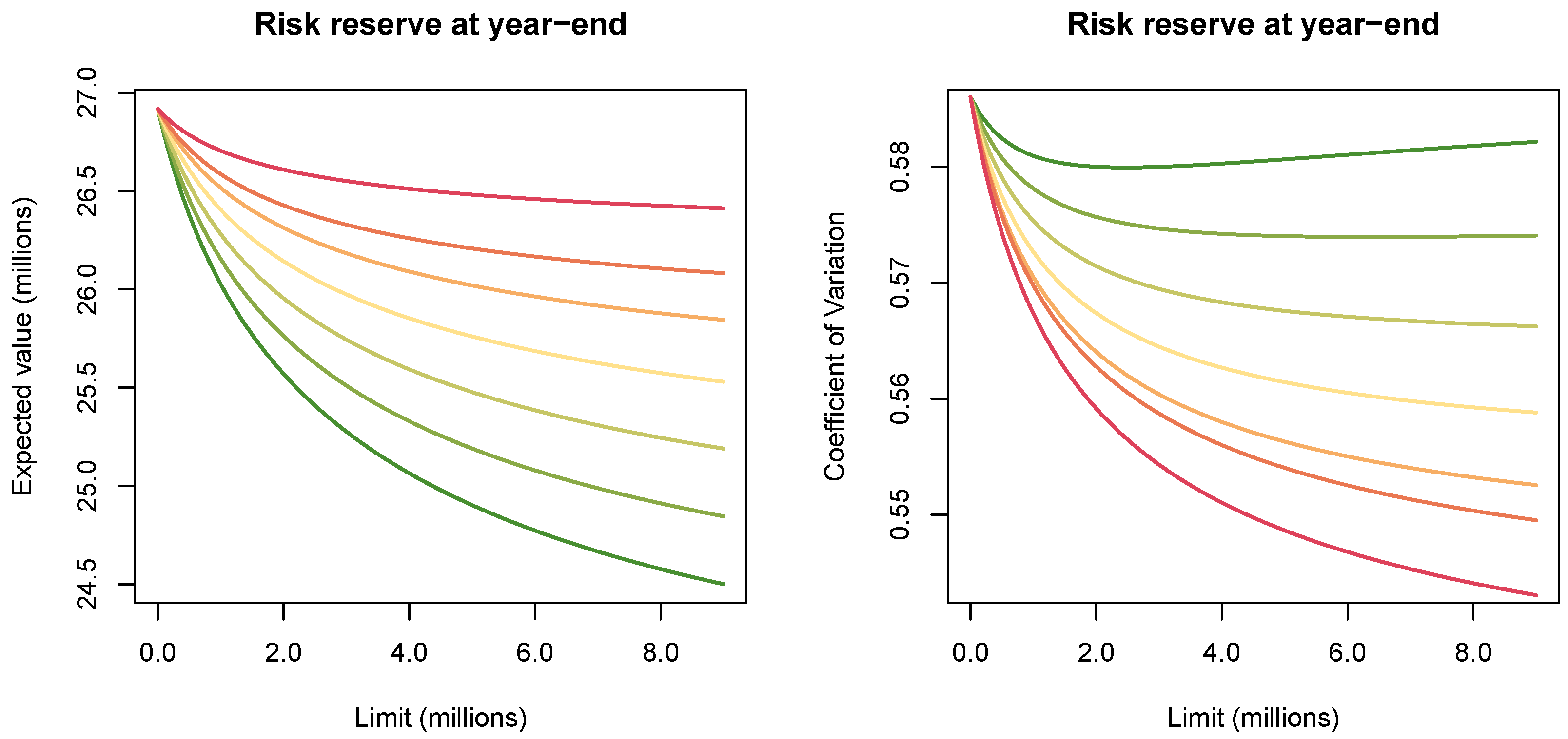
One of the possible applications of the closed-form results for mean and variance of the risk reserve that we now present consists in their use for the comparison of different reinsurance strategies and the choice of the optimal one, in a much shorter computational time and with a higher accuracy compared to a simulative approach. In Figure 1, the mean and coefficient of variation (CoV) of the risk reserve are reported for different values of limit l, all the other parameters fixed, including the deductible set equal to d = 1,000,000. Moreover, we compare these metrics for different ratings of the reinsurance company.

We can observe that, for all the values of CQS, there is a decreasing trend in the expected capital at year end for increasing limit. Indeed, the explanation is straightforward: for a fixed deductible, a higher limit implies a higher expected cost for the reinsurance company, which leads to an increase in the price of the XL treaty, reducing the insurance technical result. Comparing the expected risk reserve for different reinsurer CQSs, we can observe that the worse the reinsurer rating, the higher the insurer result. This is in line with the theoretical expectation, since a reinsurer with a worse rating should offer a lower price, on the same conditions, for compensating its higher probability of default. In Figure 1, this effect is quite strong due to the specific assumptions on the reinsurer parameters, reported in Table 4.

Analysing the CoV of the risk reserve for the different values of l, we can observe that the general effect is a decrease in the relative variability for an increase in the limit. However, just for the case of a reinsurer with CQS equal to 0, the reduction in the CoV of the insurance company is limited to a certain value of limit after which there is an increase. This is a rather peculiar dynamic, which we analyse in more detail below.

A final interesting result that we can derive from this analysis is that, under the specific assumptions that we made, the optimal choice of reinsurance strategy for the insurance company consists in ceding the risk to a reinsurer with a CQS equal to 6. Indeed, because of the strong discount that we assume, compared to the relative low probability of default, the reinsurer with the worst CQS leads to the highest expected risk reserve and lowest CoV for the insurance company compared to the other possible reinsurers. The choice of the optimal limit for this reinsurer instead does not determine a unique value but an efficient frontier where the insurance company should choose the value that better describes its risk/return trade-off preference.

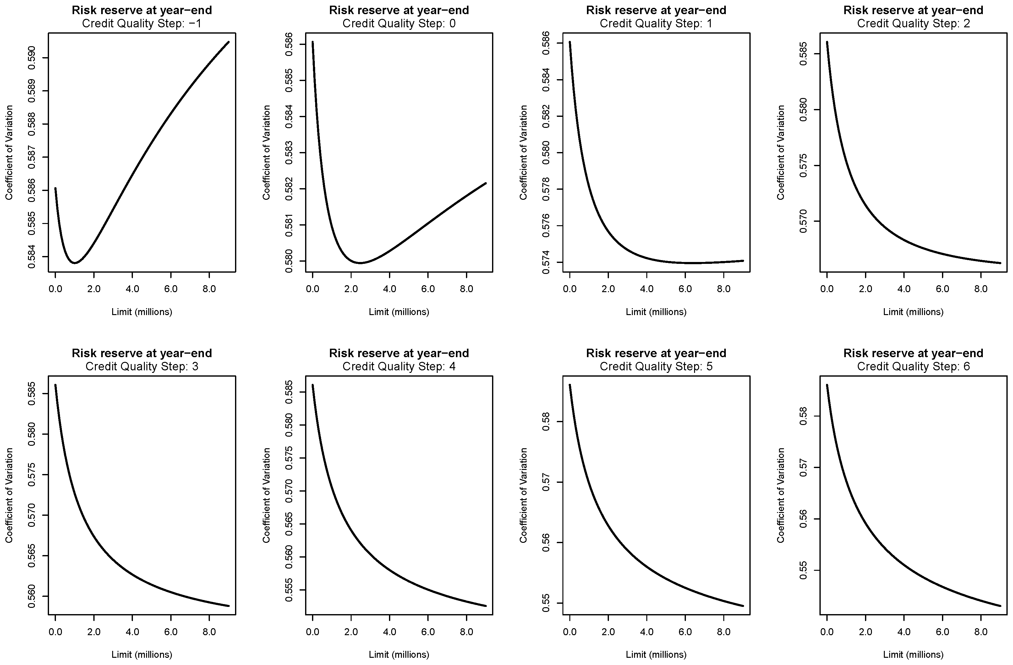
Figure 2 reports the CoV of the risk reserve for different values of limit l and for each CQS of the reinsurance company. If we are interested in a single objective optimisation consisting, for instance, in choosing the limit that minimises the CoV of the risk reserve (fixed CQS of the reinsurance company), we could analyse these figures. We observe that in the case we cede the risks to a reinsurer with a probability of default equal to 0 (CQS = $-1$), the optimal limit corresponds to 1,000,000. After this value, the CoV starts to increase, even more than the gross of reinsurance case5. The reason is that, assuming these parameters, the reduction in premium deriving from the purchase of reinsurance is less than compensated by the corresponding reduction in the standard deviation. A similar situation occurs for the case of reinsurance company with CQS equal to 0, for which the insurer reaches the minimum value of CoV for a limit of 2,500,000. For all the other CQS, there is a decreasing trend in the CoV for increasing limit; it means that for these cases, the optimal value of the limit is reached at its maximum, which corresponds to the difference between the contractual limit of the policy and the deductible.

5.3. Case of Single LoB and Multiple Reinsurers

As another step for showing the potentiality of the proposed result, we show the application of the closed formulas for mean and variance, applied for the selection of the optimal number of reinsurance counterparties for a given XL treaty. In particular, for simplicity, we consider an insurance company carrying out its activity in just one LoB and having to choose the number of reinsurers to which to cede its risks, keeping the overall deductible and limit for which it requires coverage fixed. Regarding the parameters, we assume the same characteristics of the previous numerical analysis reported in Table 1 for the GTPL LoB, while the other necessary parameters for calculating the risk reserve are instead reported in

Table 5. Parameters of the insurance company, market interest rate, and reinsurance deductible and limit (amounts in k).

P	$\mathit{\lambda }$	c	B	U	j	d	l
90,000	$12.9\%$	$32.7\%$	150,980.7	15,098.1	$1\%$	1000	2000

. Here, as anticipated, we also define the value of the reinsurance limit, because for this model we analyse the number of reinsurance companies as the variable for optimisation.

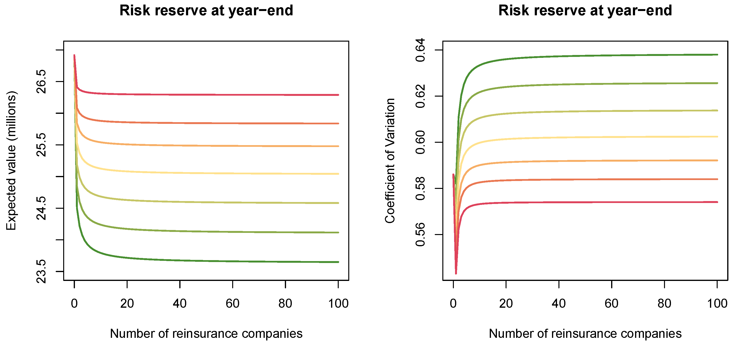
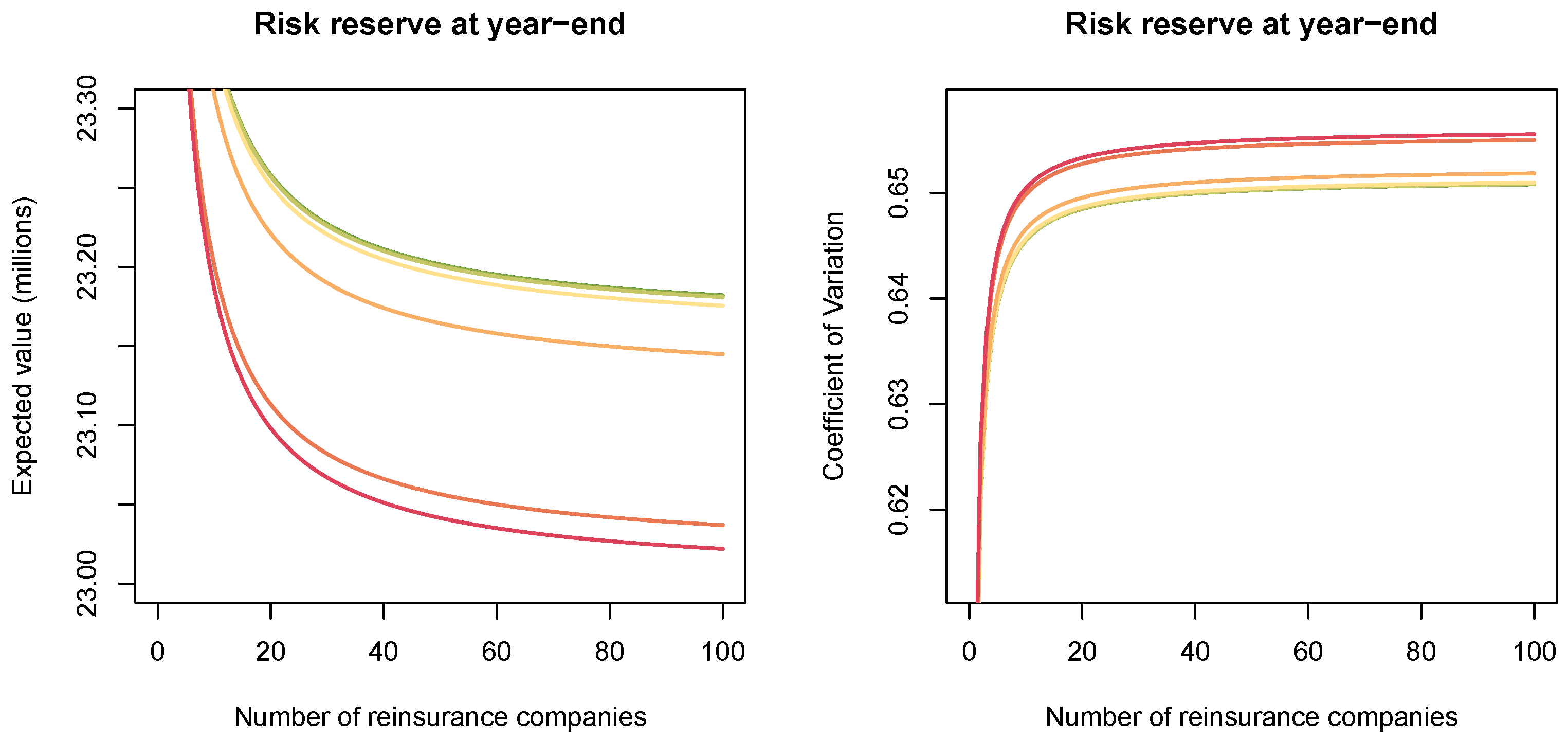
Figure 3 reports mean and CoV of the risk reserve for different values of the number of reinsurers R, having all the other parameters are fixed. We compare these metrics for different ratings of the reinsurance company.

We can observe that, for all the values of CQS, there is a decreasing trend in the expected capital at year-end for an increasing number of reinsurance companies. Indeed, for this analysis, we assume that the reinsurance companies use the standard deviation premium principle for calibrating the premium to charge to the insurer. Hence, we know that segmenting the same layer into multiple sub-layers (as in this case with multiple reinsurers) leads to an increase in the premium. In line with the theoretical expectation, comparing the expected risk reserve for different values of the CQS, it is possible to observe that a worse rating implies a higher result.

Analysing the CoV of the risk reserve for different numbers of reinsurers, we can observe an interesting dynamic. There is a decrease in the relative variability when we move from the gross of reinsurance case to the scenario with one reinsurer. After then, increasing the number of reinsurers also produces an increase in the CoV, in some cases/even higher than the gross case. This result means that, under the specific parameter assumptions that we made, the diversification of risk produced by the increase in the number of counterparties is more than offset by the reduction in the expected value.

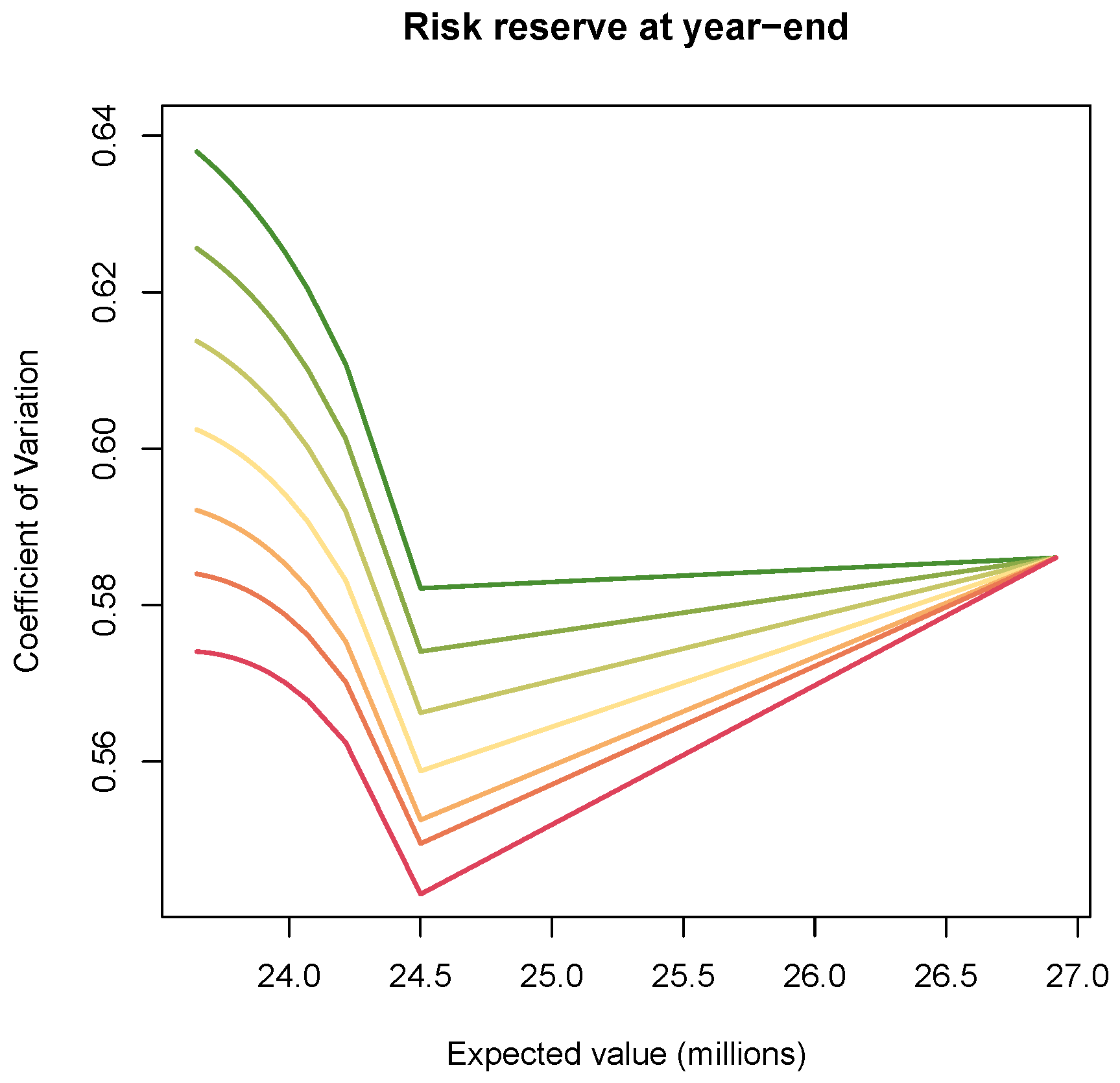
Also in this case, since we used the same parameters as in the previous section, the optimal choice of reinsurance strategy for the insurance company consists in ceding the risk to a reinsurer with a CQS equal to 6. In particular, in Figure 4 we show the frontier of reinsurance strategies for the different CQSs according to the expected value and the CoV of the risk reserve. Here, it is possible to observe that, as anticipated, the reinsurer with a CQS equal to 6 is the optimal choice in all the cases. Moreover, the reinsurance strategy that minimises the CoV is reached with a single reinsurer with a CQS equal to 6, and the value obtained is $0.54$.

Finally, in order to present the importance of considering the actual counterparty default risk and how the specific assumptions affects the choice of reinsurance strategies, in Figure 5 we report the same analysis of Figure 3, but under the assumption that the reinsurance companies offer the same price, regardless of their rating. Under this setting, the reinsurer with a CQS equal to 0 is clearly preferred since it provides the highest expected capital and the lowest relative variability to the insurance company.

5.4. Case of Multiple LoBs and Single Reinsurer

Continuing the presentation of the different applications of closed-form solutions, we consider a scenario where the insurance company carries out its activity in the 3 LoBs reported in Table 1, with their characteristics, and aims at determining the optimal limit of the XL treaty of one LoB, keeping the others fixed.

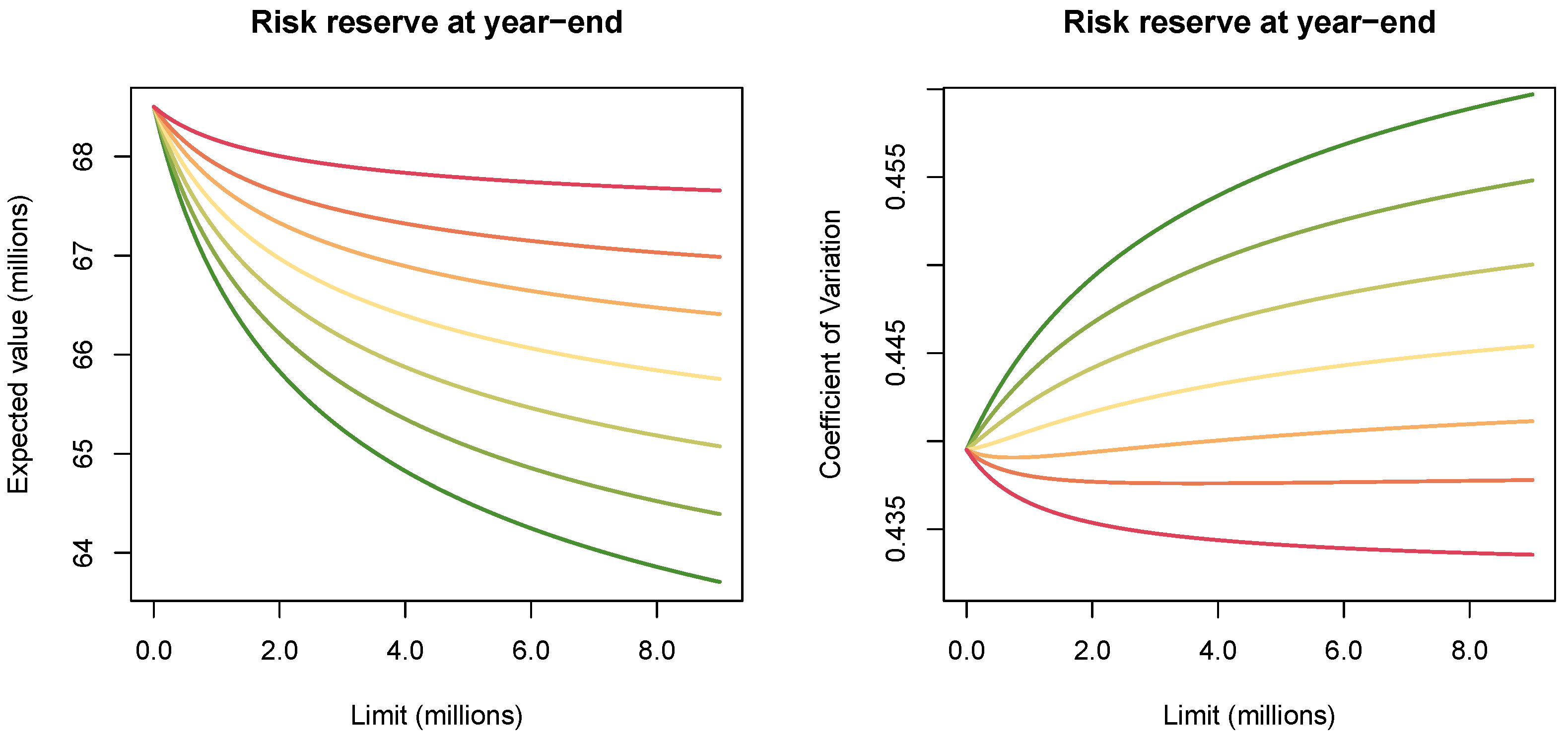
Figure 6 reports the mean and CoV of the risk reserve for various values of the XL limit of the GTPL segment, keeping all the other parameters fixed. Moreover, we compare these metrics for different ratings of the reinsurance company. In the figure on the left-hand side, we can observe that the expected value of the risk reserve decreases when we increase the XL limit. The reason is that the increasing coverage that the insurer requires costs proportionally more, since the reinsurer calibrates the premium with the standard deviation approach. Regarding the comparison between different CQSs, driven by the assumption of higher discount by reinsurers with higher CQSs, we can observe that the reinsurer with the worst CQS should be preferred since it always guarantees the highest expected risk reserve. However, in order to better determine the optimal choice, we also need to take into account a risk measure, which in this case consists in the CoV, reported in the right-hand side figure. For this metric, we can observe quite different dynamics depending on the CQS of the reinsurance company. Indeed, for reinsurers with a high rating (e.g., $CQS=1$), we observe an increasing trend in the CoV for higher values of the XL limit, meaning that, despite covering a higher portion of risk, the reduction in premium leads to a higher relative volatility compared to the gross scenario. A different dynamic is instead observed in case the risk is ceded to reinsurers with a low rating (e.g., $CQS=6$), showing a decreasing trend of the CoV for higher values of the XL limit. Moreover, looking jointly at the two graphs of Figure 6, we can determine that, given the specific parametric assumptions that we made, the reinsurer with the highest CQS should be chosen, since it always provides the highest expectation and the lowest CoV.

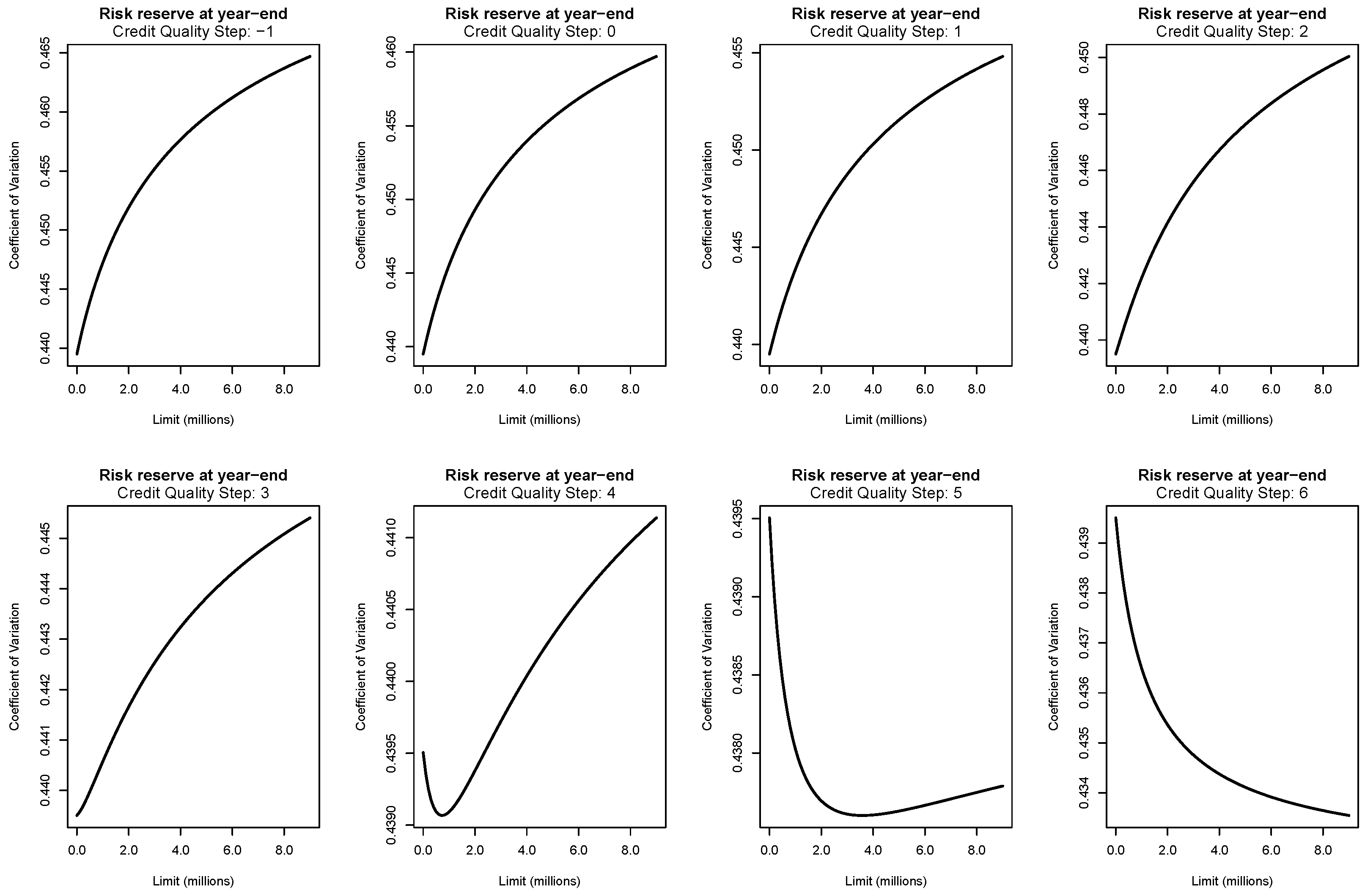
Figure 7 shows the detail of CoV of the risk reserve for different limits of the XL reinsurance for the GTPL segment. This analysis can be used in case we are interested, for instance, in the optimisation of this single metric for each CQS. Interestingly, we can observe different dynamics according to the specific rating of the reinsurance company. For CQSs from $-1$ to 3, there is an increase in the CoV from the minimum for the gross of reinsurance case to the maximum, reached at the maximum possible XL limit. Moving from a reinsurer with $CQS=-1$ to a reinsurer with $CQS=3$, we can observe that the shape of this increasing trend becomes less concave and more linear. For CQS equal to 4 and 5, instead, there is a decrease in the CoV to a minimum followed by a subsequent increase. Finally, for CQS equal to 6, the decrease in CoV as a function of the limit reaches its minimum at the extreme value of l. Hence, we determine that for CQSs from $-1$ to 3, the minimum CoV is reached for the minimum value of the limit (i.e., no reinsurance), for a CQS equal to 4 and 5, the minimum CoV corresponds to a limit of 700,000 and 3,600,000, while for a CQS of 6, the minimum CoV corresponds to the maximum value of the limit (i.e., difference between the policy limit and the deductible).

5.5. Complete Case: Multiple LoBs and Multiple Reinsurers

Finally, in this last section, we present the application of the closed-form results for the mean and variance of the complete model in the most common and realistic problem for an insurance company: the selection of the optimal reinsurance strategy. As we anticipated, an insurance company should choose a policy which produces the optimal result according to its preference structure. In practice, a typical case consists in choosing the optimal reinsurance strategy, consisting in determining the number of reinsurers, their rating, their deductible and limit for each of its LoBs, which leads to the best result, typically defined in terms of a risk and return metric.

In this context, we can take advantage of the closed-form results described in the previous section for determining mean and variance of different reinsurance strategies in a really short computational time, which would probably require weeks of computation using a simulative approach. In practice, we consider the case of an insurance company which carries out its activity in the 3 LoBs reported in Table 1 and aims at determining the reinsurance strategies that constitute the efficient frontier in a risk/return framework, using CoV and expected value of the risk reserve as measures of risk and return, respectively. Regarding the reinsurance strategy, it is constituted by the choice of the number of reinsurance counterparties, the rating of each of them and the values of deductible and limit for each of the LoBs.

In order to perform this analysis, we assume the following characteristics for the determination of a reinsurance strategy:

• 7 different levels of CQS, from 0 to 6, as reported in Table 4;
• 10 reinsurers for each CQS, for a total of 70 reinsurers from which the insurer can choose those to cede its risks, for each LoB;
• Minimum deductible of $D_{min}$ = 1,000,000 for MTPL and GTPL and $D_{min}$ = 500,000 for MOD;
• Maximum deductible of $D_{max}$ = 5,000,000 for MTPL and GTPL and $D_{max}$ = 1,000,000 for MOD.

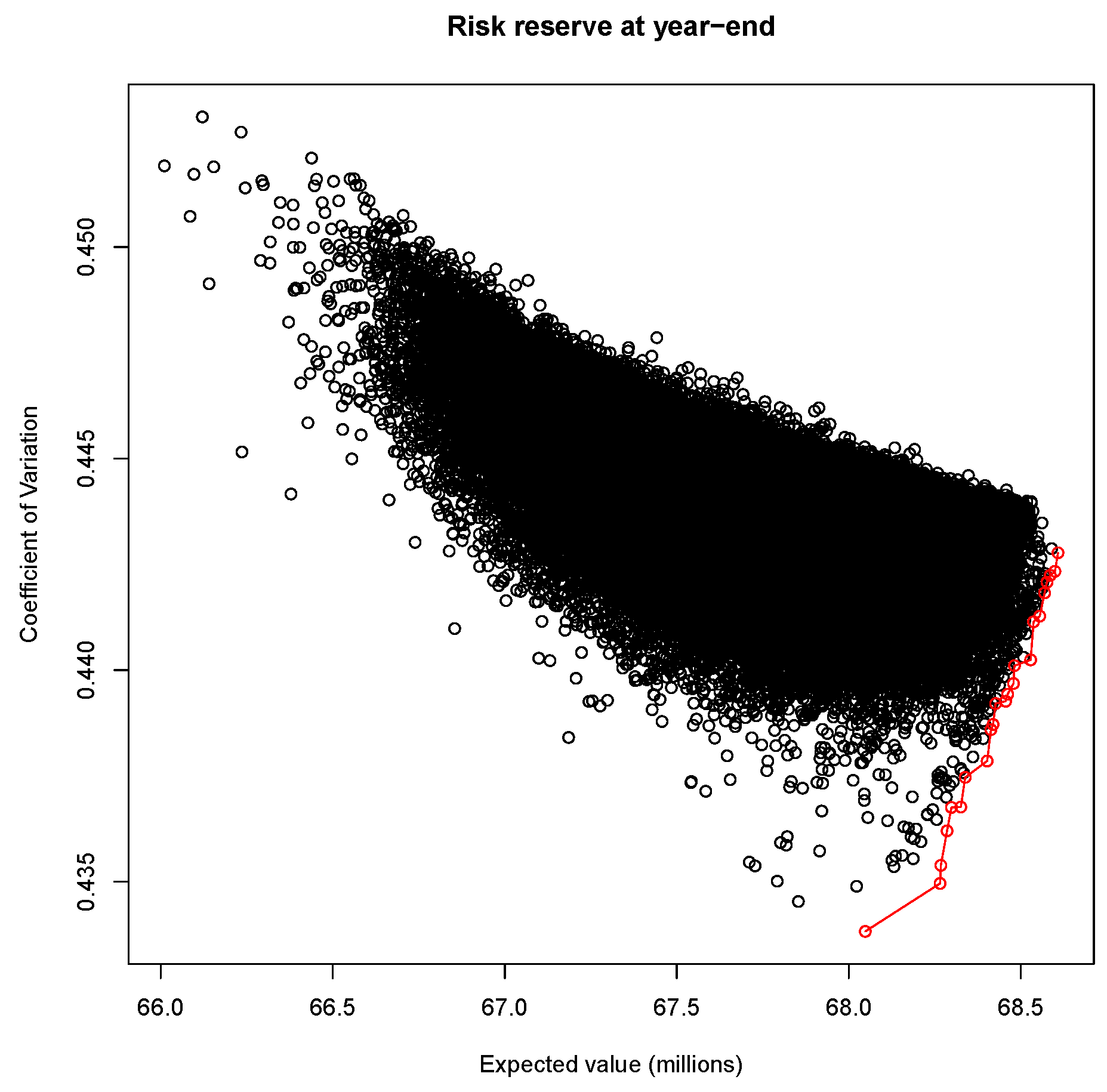
Hence, we simulate 100,000 different scenarios of reinsurance strategies according to the characteristics reported above. For each of these scenarios, we calculate the mean and variance of the risk reserve by means of (42) and (43). In this way, we are able to determine the efficient frontier of the reinsurance strategies which lead to the optimal mean/CoV trade-off, as reported in Figure 8.

As expected, we can observe that there is a high concentration of strategies in the central part of the risk/return plot, representing inefficient results. The efficient strategies, indicated in red, represent instead just a limited portion of the overall analysed scenarios. They represent the optimal strategies in the sense that, for each point in the efficient frontier, it is not possible to find another point with a higher mean and a lower CoV. However, it is not possible to determine a single optimal strategy between strategies on the efficient frontier according to the already used risk and return metrics. In practice, indeed, an insurance company chooses the optimal strategy between those on the efficient frontier according to its preference structure, typically represented by a utility function. Two extreme cases that do not require any additional elements are those where the insurance company wants to maximise the expected capital or minimise the CoV of the capital. In these cases, among the combinations on the efficient frontier, the choice should be the reinsurance strategy with the highest expected value or the lowest CoV.

In

Table 6. Characteristics of the chosen reinsurers (ID, CQS, deductible, and limit) for the MTPL segment of an efficient strategy.

ID	CQS	Deductible	Limit
36	3	2,516,769	109,567.9
38	3	2,626,337	109,567.9
62	6	2,735,905	109,567.9
17	1	2,845,473	109,567.9
45	4	2,955,041	109,567.9
32	3	3,064,609	109,567.9
9	0	3,174,177	109,567.9
33	3	3,283,745	109,567.9
64	6	3,393,313	109,567.9
39	3	3,502,881	109,567.9

,

Table 7. Characteristics of the chosen reinsurers (ID, CQS, deductible, and limit) for the GTPL segment of an efficient strategy.

ID	CQS	Deductible	Limit
61	6	4,837,945	2,165,221
69	6	7,003,166	2,165,221

and

Table 8. Characteristics of the chosen reinsurers (ID, CQS, deductible, and limit) for the MOD segment of an efficient strategy.

ID	CQS	Deductible	Limit
68	6	1,148,139	2,670,520
70	6	3,818,659	2,670,520

, we report the characteristics of the reinsurance companies of an efficient strategy.

We can observe that for the MTPL segment there is the highest number of reinsurance companies, 10, while the other 2 LoBs account for just 2 reinsurers. Moreover, as already expected from the results of a previous numerical analysis, we notice a high presence of reinsurers with a CQS equal to 6. Indeed, under the parametric assumptions that we assumed, they typically lead to the highest improvement in the relative volatility of the result. Finally, we can also notice that the insurance company chooses different reinsurers for each LoB, avoiding a concentration of risks in a single counterparty.

6. Conclusions

This paper proposes an extension of the classical risk reserve equation considering the possibility of purchasing reinsurance treaties and accounting for the counterparty default risk of the reinsurance companies. A closed-form solution for mean and variance is presented in the general case, which considers an insurance company carrying out its underwriting activity in multiple LoBs and ceding risk to multiple reinsurers with different CQSs exposed to default risk. In this way, we enriched the existing literature on the modelling of the capital of non-life insurance companies, obtaining a closed-form result of the first two moments for a framework in line with Solvency II and a real-world scenario.

The advantage of deriving mean and variance in a closed form is that they can be considered as the two main elements used to evaluate the business of a company. Indeed, from the expected capital, it is possible to derive return measures such as the Return on Equity, while the standard deviation (square root of the variance) or the CoV (ratio between standard deviation and expected value) can be interpreted as risk measures. Hence, from these two elements, we are already able to evaluate different potential strategies for the firm without requiring any simulation.

In the numerical section, we showed different applications of these closed-form results for selecting the optimal elements of a reinsurance strategy. Furthermore, we demonstrated the capability to compare a large number of complex strategies and derive the efficient frontier almost directly, as opposed to the potentially weeks of computation required by a simulation-based approach to achieve the same level of accuracy.

This extension of the risk reserve equation, with the closed-form solutions for the first two moments, should not be considered as a definitive conclusion to the problem, since it also comes with the limitation of not providing a solution for the higher moments or the quantiles. Indeed, at the moment, the main limitation of this result consists in the absence of an accurate estimation of the quantiles of the distribution, which are typically employed for determining the required capital of the company for solvency purposes. Hence, a potential area of improvement consists in the derivation of a closed-form solution for the skewness, which would allow the application of more accurate approximation methods for the quantiles of the distribution such as Normal power or Wilson–Hilferty.