Macroeconomic Dynamics in the Greek Economy during the Pre- and Post-Euro Adoption Periods

Abstract

This study examines the relationships between Greek macroeconomic variables, examining before and after the euro’s introduction as a currency. We conducted an extensive analysis from 1980 to 2019, examining various economic indicators such as government expenditure, unemployment rates, taxation, inflation, and national debt, employing causal and correlation analysis and econometric modeling with and without time-varying effects. The results revealed a significant correlation between the introduction of the euro and a tighter relationship between government spending and unemployment levels, while one more remarkable point was that higher government spending or debt reduction initiatives appeared to positively impact joblessness, particularly in the context of the euro. Our research underscored the correlation between national debt and government spending as increased debt led to reduced government expenditure and vice versa. Unemployment cited an increased impact on government spending right after the euro adoption, and on the other hand, the effect of unemployment on government spending decreased. The debt–government spending nexus was decreasing for many years before the euro adoption, while just before the euro adoption, the relationship between debt and government spending was rather stable. Finally, during the euro adoption, the effect of inflation on tax increased, while the corresponding inflation tax remained stable. Our findings have significant implications for policymakers shaping the economic strategies in Greece as they point out the necessity for stable and balanced approaches that manage government spending and debt to address unemployment effectively.

1. Introduction

The existing literature concerning Greece’s economic background provides a comprehensive approach covering different historical periods, expanding on studies focusing on the nation’s economic journey, policy structures, and key influential elements. These studies address macroeconomic theories and analyze in depth particular sectors, emphasizing the intricacies within Greece’s economic framework and its socioeconomic interactions. From the late 20th century up to the turbulence created after the global financial crisis, these studies delve into Greece’s economic progress, investigating significant milestones like economic recessions, the repercussions of the Athens 2004 Olympic Games, the European debt crisis, and the effects of fiscal, monetary, and industrial policies.

There are numerous concerns poised to surface, such as financial discrepancies, increased debts, the influence of fiscal strategies, impacts on industries, dynamics within the banking world, territorial discrepancies, effects imposed by EU measures, financial breaches, and the hurdles of transitioning to circular economy models and renewable energy sources. More importantly, these studies stress the intricate relationships between economic elements, shedding some light on the diverse nature of Greece’s economic situation as they point out its subjection to external influences and, at the same time, examine attributes such as banking dynamics, energy policies, and the impact of the broader global economic environment, underlining the complex nature that characterizes Greece’s economic dynamics.

Despite the fact that the literature showcases several studies focused on deciphering Greece’s economic history, setting the basis for holistic strategies and policies to lead the country’s economy toward resilience, sustainability, and unprecedented growth, there is a lack of in-depth evaluation of its macroeconomic dynamics, especially regarding the adoption of the euro currency. This study bridges this gap in the literature by offering useful insights into Greece’s macroeconomic landscape within the broader context of the EU’s economic background. Consequently, this work poses two research questions. First, “What is the relationship between the macroeconomic variables of Greece’s economy?” This covers also government expenditure, unemployment, taxation, inflation, and debt. And secondly, “Did the euro adoption influence that relationship?” The results suggest a correlation among numerous macroeconomic variables examined, with some cases indicating time-varying behavior around the years of the euro adoption.

2. Literature Review

The literature offers numerous works concerning the Greek economy since it has served as a prototype due to its stringent economic measures following the financial crisis. To begin with, Gogos et al. (2014) considered the years between 1979 and 2001 as great depression years, mainly due to changes in total factor productivity. They discovered that their neoclassical growth model had successfully foreseen the economic slumps in the 1980s and mid-1990s, followed by the booming recovery up until 2001, in sync with the real data. Back in 2009, Albani and Stournaras (2009) highlighted a period of substantial economic growth in Greece reinforced by domestic demand. Nevertheless, this growth phase also endured continuous financial imbalances, a budding current account deficit, and relatively high unemployment numbers, stressing the need for a stable economy taking into account both demand and supply aspects.

During the decade of 1980–1990, Karafolas and Mantakas (1996) delved into the Greek banking sector, analyzing its cost structure and prospective economies of scale. Their findings disclosed operating-cost scale economies but also the lack of total-cost scale economies, unveiling the sector’s dynamics. In 2014, Alikaj and Alexopoulos (2014) examined the Western Greece Region’s fiscal activity, realizing that the integration was minimal despite being strategically located. Thus, the chance for the tertiary sector to boost regional profit and tackle unemployment rates was emphasized. Moreover, during the 2000s period, Kasimati and Dawson (2009) examined the effect of the Athens 2004 Olympic Games, figuring non-lasting economic advances amidst the preparation of the Games but definite economic effects for the future. Furthermore, around the same period, Michaelides et al. (2013) studied the international impact on the Greek economy, demonstrating a strong correlation with the U.S. and other countries of the Economic and Monetary Union (EMU) in adopting a common monetary policy.

Pappas (2010) examined the connection between less restrictive capital accounts and macroeconomic instability, concluding that cases such as exchange rate volatility and external shocks were strongly related to fluctuations in the macroeconomic growth of Greece rather than financial openness. Trigkas et al. (2020) stressed the difficult position many established Greek companies found themselves in, highlighting the problems and selective crucial decisions these influential companies had to make, while Karfakis (2013), with his work, highlighted the important role of real credit in foreseeing shifts in real output throughout Greek business cycles. Fasianos and Tsoukalis (2023) called attention to wealth discrepancies that surfaced during the post-global financial crisis in Greece. They established that wealth inequality aggravated between 2009 and 2017, with the wealthiest 1% owning approximately as much as the poorest 50%.

Christopoulos (2003) traced no irregularities in Greece’s underground economy response to tax alterations due to taxpayers responding equally to tax inflation and cuts affecting economic policy estimates strikingly within the eurozone, while Ozturk and Sozdemir (2015) studied Greece’s economic chaos right after the global financial crisis, realizing high debt rates, budget shortages, insufficient competitiveness, and political instability. All these aspects unavoidably led to a crisis within the eurozone. Katsimi and Moutos (2010) emphasized the political and economic aspects that led to the Greek crisis, underlining a notable decrease in national saving rates and anomalies in the design of the EMU’s Stability and Growth Pact. Stamopoulos et al. (2022) stressed the meaningful input by certain sectors of the economy to GDP and employment.

Papageorgiou (2012), based on a neoclassical growth model, assessed economic policies in Greece suggesting tax regulations and policies aimed at public investment for everlasting effective impacts. At the same time, in 2022, Germaschewski and Wang (2022) investigated fiscal stabilization rules in Greece promoting balanced policies that merge productive spending and taxes for societal welfare advances. Kyrkilis and Simeon (2015) studied Greece’s industrialization and deindustrialization after WWII, pointing out sector shifts’ influences on output and employment across certain industries.

Missos et al. (2024) conducted viable research on EU austerity measures in Greece, characterizing the position of Greece as a peripheral economy within the European capitalist scheme, indicating that this status refrains the nation’s ability to forge policies, emphasizing the impact of EU-driven reorganization and suspended neoliberal amendments on Greece’s welfare system. Vinci et al. (2022) delved into Greece’s real estate market deviations, revealing discrepancies in residency costs amidst economic growth and the reduction in business activity across regions. Mensi et al. (2023), on the other hand, analyzed the existent connection between oil prices and inflation, as seen in different global economies, highlighting the role that macroeconomic factors play in creating correlations. And finally, Kapitsinis (2018) interpreted SME migration from Greece to Bulgaria after the 2007 crisis, considering societal and fiscal anomalies as the main reason for relocations.

Antoniadis et al. (2014) examined the stock returns of Greek banks amidst the financial crisis, showcasing the immediate need for larger and more profitable banks, while Konstantakis et al. (2016) assessed non-performing loans in Greece’s banking sector, illustrating the weight of macroeconomic and financial factors.

Angelopoulos et al. (2022) came up with a thorough model for a small open economy that focuses on the collective and distributional effects of public redistributive policies, as well as discovering other policies, such as increased public education expenses and higher inheritance tax rates on financial wealth, that were advantageous for leveraging income inequality, avoiding jeopardization of the macroeconomy. Passas (2023) carried out a study evaluating the capital stock in the Greek economy from 1948 to 2020 using the Perpetual Inventory Method and stressed the importance of measurement complexities in calculating macroeconomic gauges such as the capital/output ratio.

Dimakopoulou et al. (2022) assessed how effective policies relevant to the pandemic were in diminishing economic shocks in Greece due to the fact that they clarified the importance of financial support and EU aid, warning against concerns related to debt after the pandemic, while Daniel and Nam (2022) reestablished default models to define the Greek debt crisis, suggesting a justified default model that simulates existing debt behaviors in advanced economies, anticipating the outbreak of an eminent crisis with precision.

Provopoulos (2014) profiled the birth of the Greek financial crisis, stressing enhancements in external and financial anomalies and amendments in the banking sector that boosted Greece’s economic prospects. Similarly, Baltas (2013) discussed the origins of significant imbalances and high government debt in Greece, assessing existing measures taken in the eurozone crisis and proposing proactive policies to avoid similar issues. Hatgioannides et al. (2018) examined closely the neoliberal foundations of Greece’s economic crisis, shedding light on the exploitation of troika loans and supporting the need for drastic measures. This included implementing a brief use of a different currency in order to breathe life into the Greek economy within the eurozone.

Mavridakis et al. (2015a) examined Greece’s economic tactics between 2010 and 2014, underscoring its failure to encourage reinstatement and pointing out the necessity for a new plan to disentangle it from debt cycles. Tserkezos (1991) invented a way to convert yearly Greek macroeconomic data into quarterly numbers, while Goodhart et al. (2018) showcased the fact that by restructuring debt in an effective way, Greece and its creditors could seriously benefit. Kammas and Sarantides (2020) delved into how the spread of democracy influenced tax structures in Greece’s economy.

Bitros et al. (2016) explored the influence of European Monetary Union transfers and Greek domestic policies on the economy, highlighting a close relationship with the great financial crisis. Papatheodorou (1990) examined the impact of energy on Greece’s macroeconomy with the aid of simulations, while Samitas and Polyzos (2016) highlighted the devastating effects of delayed banking capital controls in Greece. Moreover, Samitas and Tsakalos (2013) analyzed the shifting associations between Greek and European markets amidst the debt crisis, whilst Beshenov and Rozmainsky (2015) suggested a model to examine fluctuations in the Greek debt crisis. Caloghirou et al. (1997) tested the replacement of determinants in Greek manufacturing by stressing out trends in input elasticity, and to add to that, Önder and Sunel (2021) examined the consequences of a Grexit scenario on the prevailing debt scheme of Greece, demonstrating inflation risk premiums and fractional bond markets.

Alogoskoufis (1985) suggested a model to examine macroeconomic policy in Greece, taking into account exchange rates, interest rates, and their influence on output and trade balance. Papatheodorou (1991) concentrated on establishing a coherent long-lasting production function for the Greek economy, essential for the comprehension of trends in the production sector. Kottis (1990) investigated the percentage of women’s activity in Greece, associated with their decline in unemployment and education, realizing concealed unemployment among women to be 2–3 times higher than officially documented.

Other recent studies, including Bitzenis and Makedos’s (2014) work, explored the integration of the shadow economy into the Greek GDP due to the unfolding crisis. As Eurostat expressed concerns about Greek debt figures, these studies also underscored the need to involve the shadow economy in GDP. Mavridakis et al. (2015b) commented on the rare position Greece found itself in where policies did not pair with the nation’s qualities, ending up questioning their effectiveness and causing a slow long-lasting period of adjustment. Christodoulakis and Kalyvitis (2000) showcased how the second Community Support Framework (CSF) impacted the Greek economy, suggesting that in order to be certain the enhancements will be long-lasting, strategic actions need to be taken immediately. Papadimitriou (1990), by applying and juxtaposing Marxian economic categories in Greece, revealed a drop in profit rates with inflated organic capital composition. Finally, Laopodis et al. (2016) discovered a coherent connection between government adjustments, tax evasion, and Greece’s budget deficit, disregarding political views, where GDP growth alleviates deficit variations.

Summing up, the literature highlights the importance of the Greek economy and various macroeconomic aspects that form the economic climate in Greece due to various reasons, some of which are the inclusion in the European Union, the financial crisis, or COVID-19, while few studies examine the relationships among these various macroeconomic factors. This work fills these gaps in the literature by employing classical and advanced econometric methods to examine the relationships among the various macroeconomic factors, using, as a point of reference, the adoption of the euro as a currency in Greece.

3. Methodology

In this work, archetypical econometric modeling is applied for causal identification, matching the works of Daglis (2022, 2023b). First, a unit root test is used: the Phillips–Perron test to be precise. If data are non-stationary, the first difference operator is applied.

Then, we proceed our analysis into causality investigation using the Granger causality.

Having y (dependent variable) and x (independent variable) in a stationary form, we test the null hypothesis that x does not Granger-cause y. One first finds the proper lagged values of y to be included in a univariate autoregression of y:

$$y_t=b_{0 }+b_1\times y_{t-1}+b_2\ast y_{t-2}+\dots +b_m\times y_{t-m}+{\epsilon }_t.$$

(1)

Lagged values of x are used to present the autoregressive model below:

$$y_t=b_0+b_1\ast y_{t-1}+b_2\times y_{t-2}+\dots +b_m\times y_{t-m}+c_p\times \dots \dots +c_q\times x_{t-q}+{\epsilon }_t.$$

(2)

In this regression, all lagged values of x are vital based on their t-statistics value, on the basis that they add explanatory power according to an F-test. Concerning the above-augmented regression, the index p is the lowest, and q is the longest lag length for which the lagged value of x is substantial. The null hypothesis is that the independent variable x does not Granger-cause the dependent variable y, while the other possible option is that x Granger-causes y.

We then investigate the macroeconomic relationships among the variables that we evidenced a causal relationship between, utilizing the Spearman correlation, testing for a probable change in strength in these relationships for the periods pre- and also post-euro adoption.

Spearman’s correlation coefficient is a non-parametric measure of rank correlation. For a sample of size n, the row scores X_i, Y_i are converted to ranks R(X_i), R(Y_i), so the Spearman coefficient is computed as

$$r_{s }=\frac{cov\left(R\left(X\right),R\left(Y\right)\right)}{{\sigma }_{R\left(X\right)}{\sigma }_{R\left(Y\right)}}.$$

(3)

Following this, based on the causality results for the unidirectional cases, we make use of an autoregressive lag-augmented distributed (ARDL) model, or a vector autoregressive (VAR) model in the case of bidirectional causality. For these cases (VAR models), we review the impulse responses, which are vital in economic modeling, as documented, among others, by Daglis and Katsikogianni (2022). A detailed description of the models employed is shown below.

$$Y_t=a+{{\displaystyle \sum }}_{i=1}^n{b}_i{Y}_{t-i}+{{\displaystyle \sum }}_{j=1}^m{d}_j{X}_{t-j}+e_t,$$

(4)

where $Y_t$ is the dependent variable, $X_t$ is the independent variable, and $e_t$ is the error term, while n is the lag order of the dependent variable and m is the corresponding value of the independent variable.

Similarly, for a VAR model:

$$Y_{1,t}=a_i+{{\displaystyle \sum }}_{i=1}^n{b}_i{Y}_{1, t-i}+{{\displaystyle \sum }}_{i=1}^n{d}_i{Y}_{2, t-i}+e_{1,t},$$

(5)

$$Y_{2,t}=c_i+{{\displaystyle \sum }}_{i=1}^n{f}_i{Y}_{2, t-i}+{{\displaystyle \sum }}_{i=1}^n{g}_i{Y}_{1, t-i}+e_{2,t},$$

(6)

where $Y_{1,t}$. and $Y_{2,t}$ are the dependent variables, and $e_{1,t}$ and $e_{2,t}$ are the error terms.

Finally, following Daglis (2023a, 2023c), we utilize a time-varying parameter specification to capture a probable change during the years, especially due to the euro adoption.

4. Empirical Analysis

The data used in this analysis are presented first. The data1 are given in annual frequency covering the period between 1980 and 2019 (Appendix B). The data span was selected based on data availability with adequate observations before and after the euro adoption since this is our point of reference for this study and this data span was the longest available for all variables. The data indicate government spending as a percentage of GDP (GovSpent), unemployment, tax revenue as a percentage of GDP (Tax), inflation, and debt as a percentage of GDP (Debt). We selected these variables as these are regarded to be of the greatest significance in depicting the macroeconomics of a state, especially Greece, which has shown macroeconomic instability in the past. The descriptive statistics of the data can be found in

Table 1. Descriptive statistics of the variables.

Descriptive Statistics	GovSpent	Unemployment	Tax	Inflation	Debt
Average	20.90	11.68	19.14	8.60	105.91
Standard Error	0.89	1.02	0.69	1.32	8.38
Median	23.00	9.50	19.75	4.43	101.40
Kurtosis	−0.56	0.56	−1.08	−1.11	−0.58
Skewness	−0.77	1.26	0.18	0.62	0.43
Min	11.00	2.70	12.30	−1.74	22.53
Max	31.00	27.50	26.90	24.68	212.38

(we also developed source code in R—Appendix A).

Based on

Table 2. Phillips–Perron unit root tests.

Variable	DF	p-Value
GovSpent_PercentGDP	−2.012	0.569
Unemployment	−2.149	0.515
TaxRevenue_PercentGDP	−2.770	0.271
Inflation	−2.087	0.539
Debt_PercentGDP	−1.464	0.784

all data are non-stationary, and thus the first-difference transformation is used. We proceed with our analysis using the Granger causality results, as displayed in the next table (

Table 3. Granger causality results.

Dependent Variable	Independent Variables_Names	F-Stat	p-Value	Lag
GovSpent	Unemployment	4.405	0.043	1
Unemployment	GovSpent	3.871	0.057	1
Tax	Unemployment	0.055	0.815	1
Unemployment	Tax	0.292	0.592	1
Inflation	Unemployment	0.700	0.408	1
Unemployment	Inflation	1.624	0.211	1
Debt	Unemployment	2.267	0.141	1
Unemployment	Debt	0.617	0.437	1
Debt	Unemployment	2.601	0.090	2
Debt	GovSpent	3.105	0.087	1
GovSpent	Debt	1.837	0.184	1
Inflation	GovSpent	1.800	0.188	1
GovSpent	Inflation	0.612	0.439	1
Tax	GovSpent	0.011	0.918	1
GovSpent	Tax	0.069	0.795	1
Tax	Debt	0.240	0.627	1
Debt	Tax	2.294	0.139	1
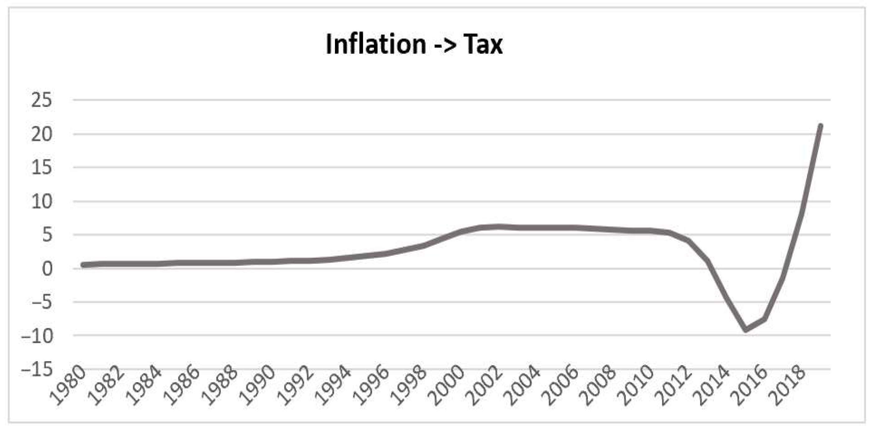
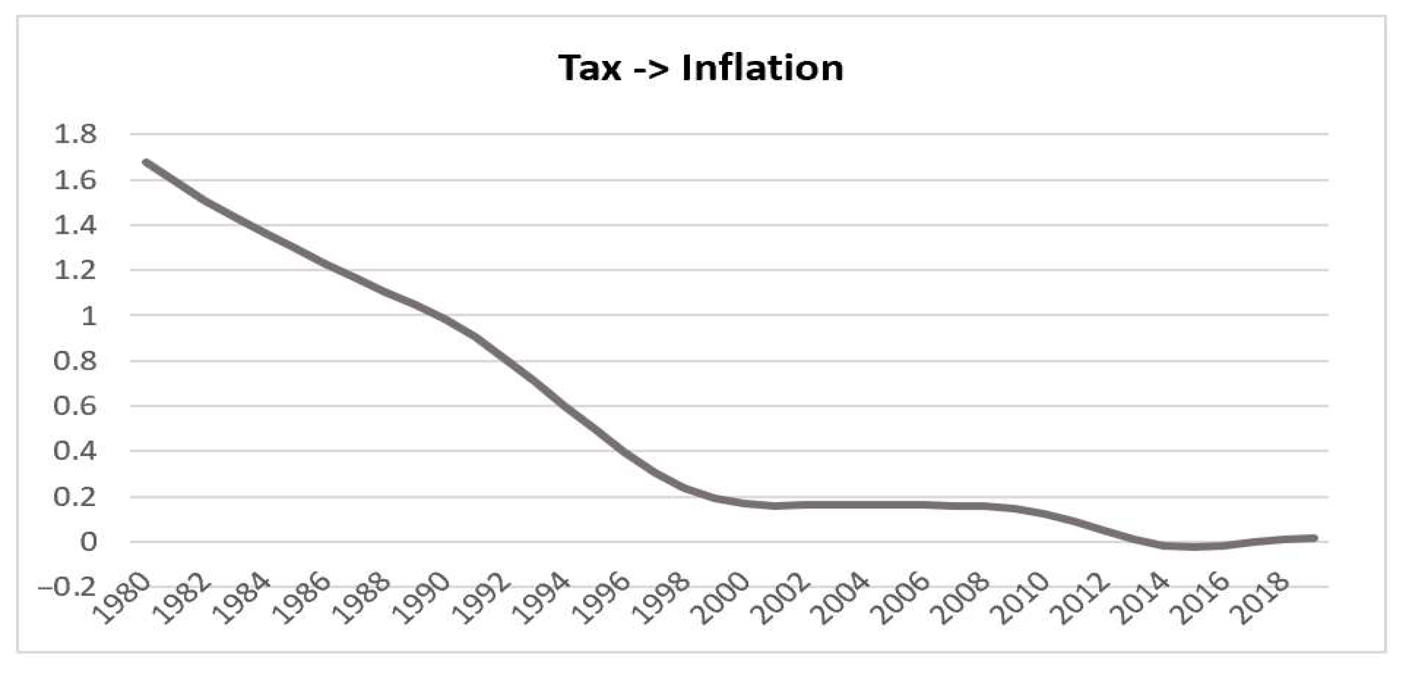
Tax	Inflation	6.842	0.013	1
Inflation	Tax	11.409	0.002	1

).

Based on Table 3, two bidirectional causal patterns are used, government spending as a percentage of GDP and unemployment. Similarly, tax revenue as a percentage of GDP and inflation are used. For these cases, a vector autoregressive model is applied. On the other hand, one-directional causalities are traced since debt as a percentage of GDP and government spending as a percentage of GDP cause unemployment.

Finally, we supply the relevant analysis for each causal case that we traced using a correlation analysis for the whole era, pre-euro era, and euro era, providing the impulse responses for the cases of VAR models or the ARDL summary in the case of one-directional causalities.

In

Table 4. Correlation results for the variables GovSpent and Unemployment.

Couples	Parameter	Corr	p-Value
GovSpent, Unemployment	Whole	−0.690	0.000
	Pre-Euro	−0.390	0.070
	Euro	−0.880	0.000

, the correlation between government spending as a percentage of GDP and unemployment is −0.690 for the whole period, and based on the p-value, the results are statistically significant. The correlation between government spending as a percentage of GDP and unemployment is −0.390 for the pre-euro period, and based on the p-value, the results are significant. The correlation between government spending as a percentage of GDP and unemployment is −0.880 for the euro period, and based on the p-value, the results are significant. We conclude that the correlation between the two variables is higher for the euro period, and that is derived from the fact that as government spending increases, unemployment decreases.

Based on Figure 1, government spending negatively affects unemployment with statistical significance, while the same stands for unemployment towards government spending. In this regard, these variables display a negative simultaneous link.

Next, we examine the time-varying character of government spending and unemployment, illustrated in Figure 2.

It is evident from the time-varying parameter (TVP) modeling there was an increase in the effect of unemployment on government spending right after the euro adoption, and on the other hand, the effect of unemployment on government spending decreased. Of course, a totally different pattern exists during the financial crisis.

In

Table 5. Correlation results for the variables Debt and Unemployment.

Couples	Parameter	Corr	p-Value
Debt, Unemployment	Whole	0.872	0.000
	Pre-Euro	0.810	0.000
	Euro	0.723	0.001

, the correlation between debt as a percentage of GDP and unemployment is −0.872 for the whole period, and based on the p-value, the results are statistically significant. The correlation between debt as a percentage of GDP and unemployment is −0.810 for the pre-euro period, and based on the p-value, the results are statistically significant. The correlation between debt as a percentage of GDP and unemployment is −0.723 for the euro period, and based on the p-value, the results are statistically significant. We conclude that the correlation between the two variables is higher for the euro period, and that derives from the fact that as government spending increases, unemployment decreases.

Based on the ARDL results, the lags in unemployment that are statistically significant demonstrate a negative sign (see

Table 6. Coefficients for the variables Debt and Unemployment.

Variable	Estimate	Std. Error	t-Value	Pr(>|t|)
(Intercept)	4.469	2.129	2.100	0.046
Debt(−1)	−0.090	0.210	−0.427	0.673
Debt(−1)	0.057	0.203	0.279	0.782
Unemployment	1.368	1.541	0.887	0.383
Unemployment(−1)	−0.415	2.148	−0.193	0.848
Unemployment(−2)	1.568	2.144	0.732	0.471
Unemployment(−3)	−3.506	2.007	−1.746	0.093
Unemployment(−4)	2.367	1.994	1.187	0.246
Unemployment(−5)	0.169	1.520	0.111	0.912

). Consequently, unemployment negatively affects debt as a percentage of GDP.

We then present in Figure 3 the TVP characteristics of this relationship, using, as a point of reference, the euro adoption.

Based on Figure 3, the time-varying effect of the unemployment–debt nexus is linear and decreasing; hence, no specific results can be derived from the euro adoption.

In

Table 7. Correlation results for the variables Debt and GovSpent.

Couples	Parameter	Rho	S	p-Value
Debt, GovSpent	Whole	−0.702	18,146.000	0.000
	Pre-Euro	−0.471	2604.800	0.027
	Euro	−0.923	1862.900	0.000

, the correlation between debt as a percentage of GDP and government spending as a percentage of GDP is −0.702 for the whole period, and based on the p-value, the results are statistically significant. The correlation between debt as a percentage of GDP and government spending as a percentage of GDP is −0.471 for the pre-euro period, and based on the p-value, the results are statistically significant. The correlation between debt as a percentage of GDP and government spending as a percentage of GDP is −0.923 for the euro period, and based on the p-value, the results are statistically significant.

To a high degree, debt has a negative sign in both levels and lags, and thus it negatively affects government spending (see

Table 8. Coefficients for the variables Debt_PercentGDP and GovSpent_PercentGDP.

Variable	Estimate	Std. Error	t-Value	Pr(>|t|)
(Intercept)	0.440	0.477	0.924	0.364
GovSpent(−1)	−0.012	0.199	−0.061	0.952
Debt	−0.096	0.034	−2.801	0.010
Debt(−1)	−0.070	0.039	−1.807	0.083
Debt(−2)	−0.036	0.036	−1.008	0.323
Debt(−3)	0.019	0.033	0.557	0.582
Debt(−4)	−0.024	0.035	−0.693	0.495
Debt(−5)	0.032	0.036	0.901	0.376

). We then present in Figure 4 the TVP characteristics of this relationship, using, as a point of reference, the euro adoption.

Based on Figure 4, the time-varying effect of the debt–government spending nexus decreased for many years before the euro adoption, while just before the euro adoption until the onset of the financial crisis, the relationship between debt and government spending was rather stable.

In

Table 9. Correlation results for the variables TaxRevenue_PercentGDP and Inflation.

Couples	Parameter	Corr	p-Value
TaxRevenue_PercentGDP, Inflation	Whole	−0.842	0.000
	Pre-Euro	−0.736	0.000
	Euro	−0.610	0.007

, the correlation between tax revenue as a percentage of GDP and inflation is −0.842 for the whole period, and based on the p-value, the results are statistically significant. The correlation between tax revenue as a percentage of GDP and inflation is −0.736 for the pre-euro period, and based on the p-value, the results are statistically significant. The correlation between tax revenue as a percentage of GDP and inflation is −0.610 for the euro period, and based on the p-value, the results are statistically significant.

Interestingly, inflation negatively affects tax revenue, while tax revenue positively affects inflation (see Figure 5). However, the first case (inflation versus tax revenue) provides only one moment of statistical significance, hence some doubt about this result. This specific direction will not be included in the derivation of the results. However, it could be an avenue for further research.

Finally, in Figure 6, we present the TVP characteristics of the relationship between tax and inflation.

The results in Figure 6 show that during the euro adoption, the effect of inflation on tax increased, while the corresponding effect of tax on inflation remained stable.

5. Discussion

This work studies the Greek economy through a macroeconomic lens, using, as a benchmark, the adoption of the euro, and thus assessing its implications across different economic indicators. More specifically, this work compares the pre-euro with the euro era, offering a detailed analysis of the consequences the euro brought on the Greek economy but also examining macroeconomic indicators like government spending, unemployment, tax revenue, inflation, and debt before and after the euro era, affirming interesting patterns in Greece’s economic reality.

Granger causality tests revealed bidirectional and unidirectional causal links among macroeconomic variables, calling attention to the patterns discovered between government spending and unemployment. They also unveiled that tax revenue and inflation demonstrated bidirectional causal relationships.

After a thorough inspection via correlation analysis, varying strengths of relationships were showcased between specific variables across different timeframes. More specifically, during the euro era, a less evident negative correlation was noticed between government spending and unemployment, while debt illustrated a stronger negative correlation with unemployment during the same period, hinting that economic changes were made possible post-euro adoption.

Further research unveiled that unemployment tended to drop whenever government spending increased or debt decreased, especially during the euro era, as the interrelation of these variables advocates subtle differences in dynamics within the Greek economy, which are probably impacted by tactics or economic shifts closely related to the euro introduction. Regarding the time-varying effects, using, as a point of reference, the euro adoption, unemployment cited an increased impact on government spending right after the euro adoption, and on the other hand, the effect of unemployment on government spending decreased. On the other hand, the time-varying effect of the debt–government spending nexus decreased many years before the euro adoption, while just before the euro adoption until the onset of the financial crisis, the relationship between debt and government spending was rather stable. Finally, during the euro adoption, the effect of inflation on tax increased, while the corresponding inflation tax remained stable.

Our results have several implications based on the economic theory and the global context. Based on the derived results, the causal relationships evidenced regarding government spending and unemployment, and tax revenue and inflation, are in line with Keynesian economic theory, particularly because government spending acts as a leverage for igniting economic activity and simultaneously reducing unemployment during eras of economic turmoil. On the other hand, changes in tax revenue and inflation may have an impact as well since they are interconnected with economic activity and monetary policy. Furthermore, according to the results, the introduction of the currency of the euro affected the economic dynamics in Greece, which in turn led to variations in fiscal and monetary policies, performing, in some way, as an exogenous shock, able to reshape the relationships of these variables. Moreover, the elevated effect of unemployment on government spending just after the euro adoption proves that this period was an era of policy responses and adjustments to the evolving economic climate. Similarly, the stability of the relationship between debt–government and government spending indicates a period of relative economic stability right before the onset of the financial crisis, stability that was partially driven by the euro adoption; however, external effects such as the global financial crisis had a major impact, destabilizing the Greek economy. Summing up, by examining the economic theory and having in mind the broader economic context, also arguing on the impact of exogenous shocks, the results contribute to the understanding of the economic dynamics of the Greek economy.

Our results are in line with the literature. More precisely, the economic dynamics of the Greek economy seem to demonstrate changes over time, especially during specific events (Kasimati and Dawson 2009). This is also evident from our work, since the correlation results, and the time-varying parameter modeling, showed that during various periods, the Greek macroeconomic relationships changed their dynamics, particularly during the period around the euro adoption. Moreover, various fiscal policies and public investments have already been argued to stabilize the economic climate in Greece (Germaschewski and Wang 2022). In this regard, during the euro adoption, Greece indeed seemed to demonstrate stability in its macroeconomics, as shown by our results. Moreover, correlations seem to change during various periods of economic and political significance, as proven by Samitas and Tsakalos (2013), which is also a finding proposed by our work. Finally, Laopodis et al. (2016) found a consistent link between government changes, tax evasion, and Greece’s budget deficit, which is also consistent with our work, since we prove that the macroeconomic relationships among the various variables examined are time-dependent, especially around the period of the euro adoption.

However, it is worth noting that most research works examine the effect of crises or negative events in the Greek economy such as the work of Samitas and Tsakalos (2013); however, no study has used the euro adoption as a point of reference. Therefore, our work contributes to the literature by expanding these results since, by answering the two research questions posed, we prove that (1) there is a relationship among the macroeconomics of Greece examined and (2) the euro adoption played a significant role in this relationship.

In addition, after the introduction of the euro in Greece, the economic landscape shifted because leaders were obliged to seriously consider and decide what changes needed to be made to adapt to this new situation because of the euro. Lastly, the study discussed how government spending and the employment sector greatly affect each other, and as a result, when the government decides upon a specific budget or commences new projects, it can influence the number of people being employed considerably.

Finally, this work demonstrates a few limitations. Analytically, data availability was one of them, since we examined this data span (1980–2019) due to data availability for all variables. Thus, the recent crisis of COVID-19 was not included in the analysis. Of course, if data become available, an approach that examines the possible effect of the COVID-19 pandemic would be of great importance. Finally, this work performs an analysis purely in a macroeconomic framework; therefore, no financial data were utilized. However, regarding the macroeconomic relationships examined and the euro adoption being utilized as a point of reference, the results are not significantly impacted by these limitations since they are evidenced by more than one method, proving also their robustness.

6. Conclusions

This research delved into the economic conditions of Greece both before and after the adoption of the euro as its currency. A broad analysis covering the years between 1980 and 2019 was conducted, closely examining different macroeconomic metrics within Greece, consisting of government spending, unemployment levels, taxation, inflation, and national debt.

According to our results, the negative correlation between government spending and unemployment during the euro era suggests that increased government spending might have contributed to lower unemployment rates, implying that fiscal policies, characterized by increased government spending, can reduce unemployment. Moreover, the stronger negative correlation between debt and unemployment during the euro era indicates that reducing debt levels could have positive effects on reducing unemployment, implying that fiscal consolidation measures to reduce government debt may have been associated with improvements in labor market conditions, with euro adoption playing a role in that too.

Turning now to the time-varying effects identified, the observed variations in the impact of unemployment on government spending post-euro adoption show a potential shift in economic dynamics, while the increased impact of unemployment on government spending immediately after euro adoption suggests that economic policies have been adjusted in response to the new currency utilization. Likewise, the debt–government and government spending relationship reveals a decreasing time-varying effect of the debt–government on spending before the euro adoption, while its stability afterward shows that the relationship between debt and government spending has been influenced by external factors such as economic reforms, particularly the adoption of the euro as a currency. Therefore, fiscal management is required to maintain stability in the debt–government spending relationship. Finally, the observed increase in the effect of inflation on tax during the euro adoption period proves the presence of adjustments in tax policies in response to inflationary pressures, while stable effects of tax on inflation show that tax policies have been less responsive to inflationary trends. In this regard, measures to ensure that tax policies are aligned with inflation dynamics are necessary to maintain macroeconomic stability, as evidenced by our case study. The findings stress the need for policymakers and politicians to come up with decisions in order to effectively manage how money, debt, jobs, taxes, and prices are interconnected, aiming to draft a solid plan that will contribute to the growth and stability of the economy.

This work provides a better view of the complexity of the economy of Greece using information derived from its macroeconomic history, showing that choices made by policymakers, especially the adoption of the euro currency, have been critical for the economic future of Greece, highlighting the significance of such events and decisions in the macroeconomic stableness of countries. This work provides avenues for further research, for example, to examine the macroeconomic performance of European countries, as well as their interrelationships, since they all perform under the same currency, or finally, to analyze how the world’s economy affects Greece or other European countries and how macroeconomic policies respond to turbulent eras.

References

- Albani, Maria, and Yannis Stournaras. 2009. A Model to Deal with Aggregate Supply and Demand Imbalances: The Case of Greece. The Journal of Economic Asymmetries 6: 15–28. [Google Scholar] [CrossRef]
- Alikaj, Mirsida, and Yiorgos Alexopoulos. 2014. Analysis of the Economy of Region of Western Greece. An Application of the Social Accounting Matrix (SAM). Procedia Economics and Finance 14: 3–12. [Google Scholar] [CrossRef][Green Version]
- Alogoskoufis, George S. 1985. Macroeconomic policy and aggregate fluctuations in a semi-industrialized open economy. European Economic Review 29: 35–61. [Google Scholar] [CrossRef]
- Angelopoulos, Angelos, George Economides, George Liontos, Apostolis Philippopoulos, and Stelios Sakkas. 2022. Public redistributive policies in general equilibrium: An application to Greece. The Journal of Economic Asymmetries 26: e00271. [Google Scholar] [CrossRef]
- Antoniadis, Ioannis, A. Alexandridis, and Nikolaos Sariannidis. 2014. Mergers and Acquisitions in the Greek Banking Sector: An Event Study of a Proposal. Procedia Economics and Finance 14: 13–22. [Google Scholar] [CrossRef]
- Baltas, Nicholas C. 2013. The Greek financial crisis and the outlook of the Greek economy. The Journal of Economic Asymmetries 10: 32–37. [Google Scholar] [CrossRef]
- Beshenov, Sergey, and Ivan Rozmainsky. 2015. Hyman Minsky’s financial instability hypothesis and the Greek debt crisis. Russian Journal of Economics 1: 419–38. [Google Scholar] [CrossRef][Green Version]
- Bitros, George C., Bala Batavia, and Parameswar Nandakumar. 2016. Economic crisis in the European periphery: An assessment of EMU membership and home policy effects based on the Greek experience. The North American Journal of Economics and Finance 36: 312–27. [Google Scholar] [CrossRef][Green Version]
- Bitzenis, Aristidis, and Ioannis Makedos. 2014. The Absorption of a Shadow Economy in the Greek GDP. Procedia Economics and Finance 9: 32–41. [Google Scholar] [CrossRef][Green Version]
- Caloghirou, Yannis D., Alexi G. Mourelatos, and Tompson Henry. 1997. Industrial energy substitution during the 1980s in the Greek economy. Energy Economics 19: 476–91. [Google Scholar] [CrossRef]
- Christodoulakis, Nicos M., and Sarantis Kalyvitis. 2000. The Effects of the Second Community Support Framework 1994–99 on the Greek Economy. Journal of Policy Modeling 22: 611–24. [Google Scholar] [CrossRef]
- Christopoulos, Dimitris K. 2003. Does underground economy respond symmetrically to tax changes? Evidence from Greece. Economic Modelling 20: 563–70. [Google Scholar] [CrossRef]
- Daglis, Theodoros. 2022. The excessive gaming and gambling during COVID-19. Journal of Economic Studies 49: 888–901. [Google Scholar] [CrossRef]
- Daglis, Theodoros. 2023a. An investigation of the impact of COVID-19 on health-related cryptocurrencies using time-varying parameters and impulse responses. Healthcare Analytics 4: 100226. [Google Scholar] [CrossRef]
- Daglis, Theodoros. 2023b. The dynamic relationship of cryptocurrencies with supply chain and logistics stocks—The impact of COVID-19. Journal of Economic Studies 50: 840–57. [Google Scholar] [CrossRef]
- Daglis, Theodoros. 2023c. The Tourism Industry’s Performance During the Years of the COVID-19 Pandemic. Computational Economics. [Google Scholar] [CrossRef]
- Daglis, Theodoros, and Maria-Anna Katsikogianni. 2022. The Repercussions of Covid-19 on the Stock Market of the Tourism Industry. Tourism Analysis 27: 77–91. [Google Scholar] [CrossRef]
- Daniel, Betty C., and Jinwook Nam. 2022. The Greek debt crisis: Excusable vs. strategic default. Journal of International Economics 138: 103632. [Google Scholar] [CrossRef]
- Dimakopoulou, Vasiliki, George Economides, and Apostolis Philippopoulos. 2022. The ECB’s policy, the Recovery Fund and the importance of trust and fiscal corrections: The case of Greece. Economic Modelling 112: 105846. [Google Scholar] [CrossRef]
- Fasianos, Apostolos, and Panos Tsoukalis. 2023. Decomposing wealth inequalities in the wake of the Greek debt crisis. The Journal of Economic Asymmetries 28: e00307. [Google Scholar] [CrossRef]
- Germaschewski, Yin, and Shu-Ling Wang. 2022. Fiscal stabilization in high-debt economies without monetary independence. Journal of Macroeconomics 72: 103398. [Google Scholar] [CrossRef]
- Gogos, Stylianos G., Nikolaos Mylonidis, Dimitris Papageorgiou, and Vanghelis Vassilatos. 2014. 1979–2001: A Greek great depression through the lens of neoclassical growth theory. Economic Modelling 36: 316–31. [Google Scholar] [CrossRef]
- Goodhart, Charles, Udara Peiris, and Dimitrios Tsomocos. 2018. Debt, recovery rates and the Greek dilemma. Journal of Financial Stability 36: 265–78. [Google Scholar] [CrossRef]
- Hatgioannides, John, Marika Karanassou, Hector Sala, Menelaos G. Karanasos, and Panagiotis D. Koutroumpis. 2018. The legacy of a fractured Eurozone: The Greek Dra(ch)ma. Geoforum 93: 11–21. [Google Scholar] [CrossRef]
- Kammas, Pantelis, and Vassilis Sarantides. 2020. Democratisation and tax structure in the presence of home production: Evidence from the Kingdom of Greece. Journal of Economic Behavior & Organization 177: 219–36. [Google Scholar] [CrossRef]
- Kapitsinis, Nikos. 2018. Interpreting business mobility through socio-economic differentiation. Greek firm relocation to Bulgaria before and after the 2007 global economic crisis. Geoforum 96: 119–28. [Google Scholar] [CrossRef]
- Karafolas, Simeon, and G. Mantakas. 1996. A note on cost structure and economies of scale in Greek banking. Journal of Banking & Finance 20: 377–87. [Google Scholar] [CrossRef]
- Karfakis, Costas. 2013. Credit and business cycles in Greece: Is there any relationship? Economic Modelling 32: 23–29. [Google Scholar] [CrossRef][Green Version]
- Kasimati, Evangelia, and Peter Dawson. 2009. Assessing the impact of the 2004 Olympic Games on the Greek economy: A small macroeconometric model. Economic Modelling 26: 139–46. [Google Scholar] [CrossRef]
- Katsimi, Margarita, and Thomas Moutos. 2010. EMU and the Greek crisis: The political-economy perspective. European Journal of Political Economy 26: 568–76. [Google Scholar] [CrossRef]
- Konstantakis, Konstantinos N., Panayotis G. Michaelides, and Angelos T. Vouldis. 2016. Non performing loans (NPLs) in a crisis economy: Long-run equilibrium analysis with a real time VEC model for Greece (2001–2015). Physica A: Statistical Mechanics and Its Applications 451: 149–61. [Google Scholar] [CrossRef]
- Kottis, Athena Petraki. 1990. Shifts over time and regional variation in women’s labor force participation rates in a developing economy: The case of Greece. Journal of Development Economics 33: 117–32. [Google Scholar] [CrossRef]
- Kyrkilis, Dimitrios, and Semasis Simeon. 2015. Greek Agriculture’s Failure. The Other Face of a Failed Industrialization. From Accession to EU to the Debt Crisis. Procedia Economics and Finance 33: 64–77. [Google Scholar] [CrossRef]
- Laopodis, Nikiforos T., Anna A. Merika, and Merika Annie Triantafillou. 2016. Unraveling the political budget cycle nexus in Greece. Research in International Business and Finance 36: 13–27. [Google Scholar] [CrossRef]
- Mavridakis, Theofanis, Dimitrios Dovas, and Spiridoula Bravou. 2015a. The Effectiveness of the Adjustment Policies Applied to the Greek Economy. Procedia Economics and Finance 19: 101–9. [Google Scholar] [CrossRef][Green Version]
- Mavridakis, Theofanis, Dimitrios Dovas, and Spiridoula Bravou. 2015b. The Results of the Adjustment Program for the Greek Economy. Procedia Economics and Finance 33: 154–67. [Google Scholar] [CrossRef][Green Version]
- Mensi, Walid, Ur Rehman Mobeen, Shawkat Hammoudeh, Xuan Vingh Vo, and Won Joong Kim. 2023. How macroeconomic factors drive the linkages between inflation and oil markets in global economies? A multiscale analysis. International Economics 173: 212–32. [Google Scholar] [CrossRef]
- Michaelides, Panayotis G., Theofanis Papageorgiou, and Angelos T. Vouldis. 2013. Business cycles and economic crisis in Greece (1960–2011): A long run equilibrium analysis in the Eurozone. Economic Modelling 31: 804–16. [Google Scholar] [CrossRef]
- Missos, Vlassis, Charalampos Domenikos, and Nikos Pontis. 2024. Hardening the EU core-periphery lines, 2009–2019: Dependency, neoliberalism, welfare reformation and poverty in Greece. Structural Change and Economic Dynamics 69: 171–82. [Google Scholar] [CrossRef]
- Önder, Yasin Kürsat, and Enet Sunel. 2021. Inflation-default trade-off without a nominal anchor: The case of Greece. Review of Economic Dynamics 39: 55–78. [Google Scholar] [CrossRef]
- Ozturk, Serdar, and Ali Sozdemir. 2015. Effects of Global Financial Crisis on Greece Economy. Procedia Economics and Finance 23: 568–75. [Google Scholar] [CrossRef]
- Papadimitriou, Dimitri. 1990. The political economy of Greece. European Journal of Political Economy 6: 181–99. [Google Scholar] [CrossRef]
- Papageorgiou, Dimitris. 2012. Fiscal policy reforms in general equilibrium: The case of Greece. Journal of Macroeconomics 34: 504–22. [Google Scholar] [CrossRef]
- Papatheodorou, Yorgos E. 1990. Energy in the Greek economy. Energy Economics 12: 269–78. [Google Scholar] [CrossRef]
- Papatheodorou, Yorgos E. 1991. Production structure and cyclical behaviour. European Economic Review 35: 1449–71. [Google Scholar] [CrossRef]
- Pappas, Anastasios P. 2010. Capital Mobility and Macroeconomic Volatility: Evidence from Greece. The Journal of Economic Asymmetries 7: 101–21. [Google Scholar] [CrossRef]
- Passas, Costas. 2023. Standardized capital stock estimates for the Greek economy 1948–2020. Structural Change and Economic Dynamics 64: 236–44. [Google Scholar] [CrossRef]
- Provopoulos, George A. 2014. The Greek Economy and Banking System: Recent Developments and the Way Forward. Journal of Macroeconomics 39: 240–49. [Google Scholar] [CrossRef]
- Samitas, Aristeidis, and Ioannis Tsakalos. 2013. How can a small country affect the European economy? The Greek contagion phenomenon. Journal of International Financial Markets, Institutions and Money 25: 18–32. [Google Scholar] [CrossRef]
- Samitas, Aristeidis, and Stathis Polyzos. 2016. Freeing Greece from capital controls: Were the restrictions enforced in time? Research in International Business and Finance 37: 196–213. [Google Scholar] [CrossRef]
- Stamopoulos, Dimitrios, Petros Dimas, and Aggelos Tsakanikas. 2022. Exploring the structural effects of the ICT sector in the Greek economy: A quantitative approach based on input-output and network analysis. Telecommunications Policy 46: 102332. [Google Scholar] [CrossRef]
- Trigkas, Mariw, Glykeria Karagouni, K. Mpyrou, and Ioannis Papadopoulos. 2020. Circular economy. The Greek industry leaders’ way towards a transformational shift. Resources, Conservation and Recycling 163: 105092. [Google Scholar] [CrossRef]
- Tserkezos, Dikaios E. 1991. A distributed lag model for quarterly dlsaggregatmn of the annual personal disposable income of the Greek economy. Economic Modelling 8: 528–36. [Google Scholar] [CrossRef]
- Vinci, Sabato, Fransesca Bartolacci, Rosanna Salvia, and Luca Salvati. 2022. Housing markets, the great crisis, and metropolitan gradients: Insights from Greece, 2000–2014. Socio-Economic Planning Sciences 80: 101171. [Google Scholar] [CrossRef]