Abstract
This paper proposes a new approach to estimating the minimum variance hedge ratio (MVHR) based on the wild bootstrap and evaluates the approach using a spectrum of conservative to aggressive alternative hedging strategies associated with the percentiles of the MVHR’s bootstrap distribution. This approach is suggested to be more informative and effective relative to the conventional method of hedging solely based on a single-point estimate. Furthermore, the percentile-based MVHRs are robust to influential outliers, non-normality, and unknown forms of heteroskedasticity. The bootstrap percentile-based hedging strategies’ effectiveness is compared with those from the naïve method and the asymmetric DCC-GARCH model for a range of financial assets and commodities. The bootstrap percentile-based hedging technique is identified to outperform its alternatives in terms of hedging effectiveness, downside risk, and return variability, suggesting its superiority to other methods in both the literature and in practice.
Keywords:
minimum variance hedge ratio; wild bootstrap; DCC-GARCH; hedging effectiveness; heteroskedasticity; stochastic dominance JEL Classification:
C58; G13
1. Introduction
The optimal hedge ratio (or the minimum variance hedge ratio; MVHR) is widely adopted in financial risk management by both academics and practitioners. Derivative instruments, such as futures contracts, are crucial to a diversified portfolio in controlling and reducing the risk associated with unfavorable price changes. Since the first establishment of the futures market as part of the Chicago Mercantile Exchange in 1975, many studies on estimating the optimal hedge ratio and evaluating its effectiveness have been published (Chen et al. 2003; Chen et al. 2014; Wang et al. 2015; Markopoulou et al. 2016; Park and Shi 2017; Chen et al. 2021). By taking a position guided by the MVHR, an investor can effectively hedge the risk associated with price changes of an underlying asset. Ederington (1979) presents the earliest empirical study of the optimal hedge ratio as a means of risk minimization.
While the conventional method of estimating the MVHR is based on the ordinary least-squares (OLS) technique due to its simplicity and easy implementation, a number of new alternatives have been proposed in the literature, including the vector error-correction (VEC) model (Kroner and Sultan 1993; Li 2010), the generalized autoregressive conditional heteroskedasticity (GARCH) model (Caporin et al. 2014; Chang et al. 2013; Hsu et al. 2008; Ku et al. 2007; Lien et al. 2002; Park and Jei 2010), the Markov regime-switching method (Alizadeh and Nomikos 2004; Chen and Tsay 2011; Lee 2009, 2010; Lee and Yoder 2011; Su and Wu 2014), and the quantile regression method (Lien et al. 2016; Shrestha et al. 2018). These new methods are designed to overcome the shortcomings of the OLS-based method under non-normality and heteroskedasticity, which are the salient features of financial data. However, whether these new methods provide superior hedging over the OLS-based method has not been fully confirmed, in terms of hedging effectiveness and variance reduction. A number of studies find evidence that the OLS-based method does outperform these newly proposed methods: see, for instance, Lien (2009) and Lien and Shrestha (2008). As Maharaj et al. (2008) and Moosa (2017) recently pointed out, there is no evidence that econometric sophistication, in terms of elaborate model specification and superior estimation method, has boosted hedging effectiveness. Wang et al. (2015) provide an interesting finding that the naïve strategy1 is hardly outperformed by an advanced model under the minimum variance framework. This can be partly explained by estimation error and model misspecification considerations, as a small change in data quality and model specification can cause a complicated model to fail.
A notable feature of previous studies is that they rely solely on the point estimators for the optimal hedge ratio. A point estimator produces a single number as an estimate of the unknown population value. Although it may represent the most likely value from a sampling or predictive distribution, it carries no information about the degree of intrinsic uncertainty associated with estimation or prediction. As Chatfield (1993) points out in the forecasting context, an interval estimator is more informative by offering a range of possible alternatives or contingencies with a prescribed level of confidence. More importantly, Kim and Robinson (2019) demonstrate that hypothesis testing based on the interval estimator provides significantly improved inferential outcomes than those based on a single-point estimate. For this reason, one may justifiably argue that risk analysis based solely on a point estimate of the MVHR is of limited usefulness. By presenting an interval—or the percentiles within—for the optimal hedge ratio, a researcher or investor is able to conduct better-informed hedging and a more detailed risk analysis, taking full account of the degree of estimation uncertainty. Moreover, they can consider a range of possible scenarios based on a group of alternative MVHR values. For example, a number of hedging strategies within a 95% confidence interval for the optimal hedge ratio (e.g., the 25th, 50th, and 75th percentiles) can be considered.
In this paper, we contribute to the literature by proposing a new method of hedging based on the interval estimation of the MVHR. As it is OLS-based in nature, our proposal does not represent an econometric sophistication; instead, it relies on a non-parametric method of interval estimation. While it is possible to construct an OLS-based interval or percentile estimator for the optimal hedge ratio using a normal approximation, such estimators are likely to show undesirable properties in the presence of strong non-normality and heteroskedasticity in financial data (see, for example, Kim 2006). For example, an interval estimator based on a normal distribution is always symmetric around the value of the optimal hedge ratio, fails to capture the high degree of volatility of financial data, and may be subject to the effects of influential outliers. For this reason, we propose the wild bootstrap method (Davidson and Flachaire 2008) to estimate a confidence interval or percentiles for the optimal hedge ratio. The wild bootstrap is a non-parametric method of approximating the sampling distribution of a statistic based on data resampling. It is well known that a superior alternative should be provided to the conventional normal approximation when the data show unknown forms of (conditional) heteroskedasticity (Kim 2006). This paper conducts extensive empirical analyses to evaluate the hedging effectiveness based on the wild bootstrap percentiles, in comparison with the strategies based on the dynamic conditional correlation (DCC-GARCH) model with an asymmetric specification and the naïve method. Furthermore, we consider two alternative wild bootstrap procedures, i.e., one based on resampling the residuals of a regression, and the other resampling the pairs of observations. Our paper presents an innovative but simple non-parametric approach, which is different from the semi-parametric quantile regression methods used by Lien et al. (2016) and Shrestha et al. (2018). Their estimated quantile hedge ratios are based on the pairwise spot–futures quantiles independently. The hedging effectiveness is thus defined for an effective estimation of the hedge ratio for a given quantile. The major drawbacks of the quantile regression method are the complicated estimation methods required and the potential problem of quantile crossing (Waldmann 2018).
Using daily spot and futures price indices of multiple assets from 1980 to 2020 with a dynamic out-of-sample analysis framework, we find that the hedging strategies based on percentiles of the optimal hedge ratio’s bootstrap confidence interval outperform those based on the naïve hedge and the DCC-GARCH model in terms of hedging effectiveness, downside risk, and hedged return variability. Note that these percentiles are within the inter-quartile range of the bootstrap distribution, which is highly likely to cover the true value of the optimal hedge ratio. In addition, they have the desirable property of not being affected by possible extreme values. It is also found that the optimal hedging based on the pairs’ bootstrap is marginally better than that based on the residual bootstrap. Our findings hold when we perform robustness checks with stochastic dominance tests and various estimation windows. To the best of our knowledge, this approach is not yet examined in the literature. This paper is organized as follows. Section 2 presents a brief literature review. Section 3 provides the methodological details. Section 4 presents the data details and Section 5 presents the empirical results. Finally, Section 6 concludes the paper.
2. Literature Review
Chen et al. (2003) conducted a survey of different optimization functions and techniques to estimate an optimal hedge ratio. They conclude that, in general, there is no particular optimal hedge ratio that is significantly superior to the alternatives. According to Chen et al. (2014), numerous studies have been conducted to provide a solution to the risk-minimizing function of the MVHR. Nonetheless, the conclusion of which estimation method has the best hedging effectiveness remains a mixed opinion based on an out-of-sample evaluation basis. It is suggested that the major cause of these mixed results is the estimation error (Lien and Shrestha 2008).
From the in-sample analysis, the VEC hedging model with the GARCH error structure employed in Kroner and Sultan’s work (1993) is reported to be the best currency hedging strategy based on 4.5 percent and 1.5 percent variance reduction compared to the naïve and OLS models, respectively. With regard to currency hedging, Ku et al. (2007) documented that the estimation of hedge ratios using the dynamic conditional correlation (DCC–GARCH) model can reduce 0.14 percent of the variation in the unhedged portfolio relative to the constant OLS model. This is reported as the second-most-effective strategy, followed by the VEC and constant conditional correlation (CCC-GARCH) models. Park and Jei (2010), upon evaluating the hedging effectiveness for corn and soybean spot and futures prices, conclude that the incorporation of asymmetry and flexible distribution specification in the DCC-GARCH model cannot yield a better hedge outcome compared to the OLS hedge ratio, since the variance reduction benefits are relatively small. This finding is consistent with the study of Lien et al. (2002), which compares the CCC-GARCH and constant OLS approaches to hedging a spot position with different corresponding futures indices on currency, commodities, and equity securities. They also agree on similar hedging benefits among the models. In an effort to document the effect of the Euro sovereign debt crisis on currency hedging, Caporin et al. (2014) conclude that static OLS estimates for hedging strategy were appropriate during the calm (non-crisis) period and after the European Central Bank intervened. However, the authors assert that the exponential weighted moving average filter technique outperforms several other multivariate GARCH models and the static OLS model in terms of hedging effectiveness in the aftermath of the failure of the Lehman Brothers in 2008.
By using the Markov regime-switching (MRS) model, Alizadeh and Nomikos (2004) report a new technique for estimating the hedge ratio, which depends on prevailing market conditions and is also free from the non-trivial persistence effect of the distant past volatilities in the GARCH models. Although MRS ratios outperform the others as indicated in the in-sample analysis, the results from the out-of-sample analysis are mixed. In particular, the MRS ratios provide better variance reduction for the FTSE 100 hedge, but not for the S&P 500 index in comparison with the GARCH and constant OLS hedging estimates. Following this stream, Lee and Yoder (2011) and Su and Wu (2014) combine the MRS with the GARCH models (BEKK and DCC, respectively) to allow the parameters to vary over time and be state-dependent. Thus, the optimal hedge ratio is estimated from the conditional second moments of the spot and futures series that are dependent on the market states. They find better in-sample performance with the new approach, but only marginal dominance in the out-of-sample analysis in comparison to the benchmark strategies based on no hedging and the constant OLS hedge ratio. The variance reductions for hedging nickel and corn in Lee and Yoder (2011), and the S&P 500 and Nikkei 225 indices in Su and Wu (2014), are reported to be within the 0 to 2% range. Park and Shi (2017) demonstrate an innovative approach to estimating the MVHR by the MRS with trading pressures in the energy and metal commodity markets. However, the reported out-of-sample results for individual commodities do not show a significant improvement of their model over a simpler one such as the OLS or the naïve hedge in terms of variance and downside risk reduction.
In the aforementioned studies, the evidence that the alternative techniques for the MVHR estimation outperform the OLS approach has been modest in the out-of-sample analysis. This raises a question regarding the effective predictability of the proposed models, and the superiority of their time-varying properties as opposed to the static OLS model for estimating the optimal hedge ratio. Based on similar concerns, Lee and Yoder (2011) implement the statistical testing of forecasting superiority of the best model over a given benchmark, for instance, regime switching–GARCH compared to the traditional GARCH and the constant OLS models. They report that the tests for forecasting superiority among these methods are not statistically significant via White’s method for data-snooping reality check (White 2000). Notably, by using model confidence set tests for various econometric models, Wang et al. (2015) found that there is no outstanding model clearly outperforming the naïve strategy. However, the naïve hedge is significantly outperformed by the OLS-based hedge for some futures markets when the model parameters are known to a hedger ex ante.
Generally, the most popular methodology employed in recent studies are the GARCH-class models, which are able to capture dynamic relationships between the spots and futures, while the constant approaches, such as the static OLS model or the naïve strategy, fail to capture such relationships. The rationale for employing the GARCH models is the fact that high volatility in one period tends to have persistent effects in the following periods. However, convergence is also a typical problem in estimating the GARCH models. Additionally, Brooks et al. (2011) conclude that the multivariate GARCH models at best have provided a very modest enhancement for hedging effectiveness in an out-of-sample analysis. This assertion can be re-examined by reviewing reported tables of variance reduction and hedging effectiveness by employing various methods against a specific benchmark in many studies within the related literature. The reported differences in hedging improvement among the models are minor and the estimated hedge ratios appear to be slightly different. Thus far, the main disadvantage of the OLS method is that it fails in capturing the time-varying nature of the relationship among financial time series. Furthermore, the OLS assumptions are normality and constant variance of financial returns for statistical inference. Despite these shortcomings, the OLS-based MVHR is still utilized universally by financial professionals due to its computational efficiency and simplicity. As mentioned earlier, past studies rely exclusively on the point estimates of the MVHR generated from the alternative models. They report empirical results on the hedging effectiveness that are often mixed and inconclusive. This is possibly due to the above fact that the degree of uncertainty associated with the optimal hedging ratio estimation is not reflected in their evaluation. In this paper, we propose the adoption of percentile-based optimal hedging using the wild bootstrap method. The hedging strategy is based on the simple OLS regression and conducted in a time-varying framework using rolling sub-sample windows. The wild bootstrap provides estimation and statistical inference for the MVHR robust to non-normality and heteroskedasticity issues.
3. Methodology
In this section, we present the methodological details, including the wild bootstrap methods and the asymmetric DCC-GARCH model for the optimal hedge ratio. The measures for the hedging effectiveness are also discussed.
3.1. Background
The hedge ratio can be interpreted as a dollar amount in futures contracts taken by an investor or a hedger to protect against the risk of any loss from holding every one dollar in the spot market. Particularly for hedging purposes, the position in a futures contract should be opposite to the position in the spot market. Price changes in the spot and futures positions constitute the hedged return, which can be expressed as
where is a vector of the hedged portfolio’s returns; is a vector of spot returns of a risky asset; is a vector of futures contract returns of the risky asset; is the hedge ratio reflecting the size of futures contracts that needs to be entered into for the purpose of hedging the risk of USD 1 in the spot market. Note that each vector of the above returns has a length of T, which denotes the sample size.
The variance of the hedged return in (1) is as follows:
To minimize the variance of the hedged return in (2), a hedge is established using futures contracts with a size determined by the optimal hedge ratio, which is the so-called MVHR and is given by
The conventional approach uses the estimate of based on the regression of the form
The OLS estimator for β in (4) is expressed as
where the sign ′ refers to the transpose of the corresponding vector.
3.2. Hedging with Wild Bootstrap Percentiles
Efron (1979) proposed a bootstrap method for approximating the sampling distribution of a statistic in a non-parametric way by repeated resampling of the observed data. However, the true data-generating process (DGP) of the observed data cannot accurately be imitated in the bootstrap DGP if the form of heteroskedasticity is unknown. The wild bootstrap (Liu 1988; Mammen 1993) is a bootstrap method designed for data with unknown forms of heteroskedasticity, which have been shown to be asymptotically valid (Cribari-Neto and Lima 2009; Cribari-Neto et al. 2007; Davidson and Flachaire 2008; Flachaire 2005).
We contribute to the related literature by estimating distributions of the MVHR with the wild bootstrap, which is a non-parametric method and does not require prior assumptions for the heteroskedasticity and normality in the disturbance term of Equation (4). We thus examine percentiles within a confidence interval, which covers the true value of the MVHR with a prescribed level of confidence. By constructing the confidence interval and its percentiles for the MVHR, the degree of estimation uncertainty is explicitly presented. Firstly, the wild bootstrap based on residual resampling is considered, and it is employed in conjunction with the heteroskedasticity-consistent covariance matrix estimator (HCCME), as proposed in Flachaire (2005), Davidson and Flachaire (2008), and Cribari-Neto and Lima (2009). Additionally, we employ the wild bootstrap based on resampling the pairs of observations. The former bootstrap method assumes that in regression (4) is exogenous and uncorrelated with the disturbance term, while the latter assumes that it is random. The pairs’ bootstrapping process considers the potential endogeneity problem, when both and are likely to be driven by the same market shocks. The two wild bootstrap methods are proposed as alternatives for the percentile-based hedging strategy.
The wild bootstrap based on residual resampling can be described as follows:
- Step 1: Estimate the optimal hedge ratio given in (5) for the regression (4).
- Step 2: Draw a bootstrap sample () based on for each ith observation from 1 to T:where is resampled data of the spot returns, is a independent random variable with zero mean and unit variance, and is the transformed residual from the regression (4) robust to heteroskedasticity2.
- Step 3: Compute the new estimate of the hedge ratio with the bootstrap sample () (for i = 1, …, T) following the regression (4).
- Step 4: Repeat Steps 2 and 3 many times, say B, to form the bootstrap distribution of for .
- Step 5: The (1 − α)100% wild bootstrapping confidence interval is constructed with the lower limit and upper limits representing the 0.5α percentile and (1 − 0.5α) percentile, respectively, of the bootstrap distribution . The percentiles within the confidence interval can be estimated in a similar way. The number of bootstrap iterations B is set at 1000.
The wild bootstrap based on resampling the pairs is identical to the above-mentioned procedure, except in Steps 2 and 3, where resampling and estimations are conducted as ; and is the OLS estimator from (for i = 1, …, T).
Considering and , where X and Y are random variables, the variance and covariance of resampled data X* and Y*, conditional on X and Y, respectively, can effectively replicate those of X and Y. That is,
A choice should be made for the distribution for . In this paper, we use Mammen’s (1993) two-point distribution:
which is well known for giving higher-order refinements.
In this study, we construct the 95% confidence interval of the MVHR, paying attention to the 10th, 25th, 50th, 75th, and 90th percentiles. Hedging strategies are then produced based on the percentile hedge ratios. A hedged position based on an upper percentile may be regarded as an aggressive strategy, whereas that based on a lower percentile may be considered a conservative one. The 50th percentile (median) hedging position may be regarded as a neutral strategy. We argue that these percentile-based hedging strategies effectively provide different scenarios under different market conditions, since the interval will be tighter in normal times, but wider under turbulent market conditions. As a result, these hedging strategies are much more informative than the one based on a single-point estimate of the hedge ratio to seek protection against the hedged return fluctuations.
3.3. Hedging Based on the DCC-GARCH
As an alternative to the wild bootstrap, we use the bivariate DCC-GARCH(1,1) model developed by Engle (2002), which is widely used in the prior literature. The model has been popular due to its superiority to the OLS approach in considering time-varying conditional variance and covariance of the spot and futures returns. Notably, there is strong evidence in the previous literature that past volatilities have leverage effects on financial asset returns (Black 1976; Christie 1982); in particular, the effect is observed to be larger for the aggregate market index returns (Tauchen et al. 1996; Andersen et al. 2001). On this basis, the methods of Glosten et al. (1993) and Park and Jei (2010) are followed to employ an asymmetric version of the DCC-GARCH(1,1) model. The objective is to capture asymmetry in the volatility specification of the asset returns in estimating the dynamic relationship between the spot and futures returns. This model is defined as follows:
where is the dynamic conditional covariance matrix. is the vector of standardized residuals of the spot and futures returns. is the dynamic conditional correlation. is the unconditional variance matrix of . It is the indicator of the leverage effect of the past volatility on asset return, It = 1 when < 0 and otherwise 0. measures the asymmetric effect of the shocks on the dynamic conditional correlation and is the element-by-element product operator and . Hence, the time-varying hedge ratio can be calculated based on the conditional covariance matrix from the asymmetric DCC-GARCH(1,1) model, as follows:
3.4. Computational Details and Evaluation of Hedging Strategies
To conduct the hedging with time-varying estimators, we adopt the rolling sub-sample window of a 1-year trading period3 for both the wild bootstrap and the DCC-GARCH(1,1) model. From each sub-sample window, one-step ahead prediction from the DCC-GARCH(1,1) model is generated along with the wild bootstrap percentiles. To compare the predictive ability of the alternative strategies, the hedged portfolios are constructed by combining the long position in the spot market and the short position in the futures market from all windows. These hedging strategies are evaluated in terms of variance reduction, downside risk, and the overall riskiness feature of the hedged return distributions.
Conventionally, the hedging effectiveness of the strategies is measured by the percentage decrease in the return volatility of the hedged portfolio relative to that of the unhedged portfolio. An optimal hedging strategy under the minimum variance framework is expected to have a relatively stable hedge ratio and provide the largest variance reduction from the unhedged position, which is the purely long position in the spot market in this study. The hedging effectiveness (HE) is given by
where Var(U) and Var(H) denote variances in the unhedged return and hedged return, respectively. Here, the semi-variance (SV) is used to capture the average squared deviation of the observations below the mean of the hedged returns. It can be written as follows:
where m is the number of hedged return observations Xi below the average . By comparing the SV values across the proposed hedging strategies, a strategy that may potentially expose an investor to higher downside risks or substantial losses can be identified. It provides information regarding which of the available strategies is safer in situations of adverse market conditions or situations of high volatility in market movements. In addition to these measures, the inter-quartile range (difference between the 3rd and 1st quartiles) and 95% range (difference between the 97.5th and 2.5th percentiles) of the hedged return distributions are compared.
As a robustness check, we perform stochastic dominance (SD) tests to compare the overall riskiness feature of the hedged return distributions among the alternative strategies. The first and the second orders of SD tests have been widely applied in economics and finance studies (Chang et al. 2015; Liu 2016). SD testing does not require a prior assumption but considers higher moments of the data distribution. In line with the objective of financial risk managers, SD test is employed to detect which hedging strategy produces the least volatile returns. Let us consider two different hedging strategies with and as cumulative distribution functions (CDFs) where it is desirable to maximize z, denoting the value of the hedged return. The first-order test of SD is defined as for all z. That is, the CDFs of the strategy B’s hedged returns is to the right of that of strategy A. In this case, strategy B is said to first-order stochastically dominate strategy A or . This dominance order means strategy B always produces a higher average return with lower risk than strategy A. The second order is defined as if for all z. The is the necessary condition for , which indicates that the has a thicker left tail than and thus shifts to the left of . When strategy B is said to second-order stochastically dominate strategy A, it is implied that strategy B involves less risk than strategy A. Therefore, strategy B is more attractive to the financial risk managers and the hedgers. When there are no CDFs stochastically dominating another, the relationship is said to be inconclusive.
We employ the statistical test for SD proposed by Barrett and Donald (2003). The authors based their study on the Kolmogorov–Smirnov-type tests to compare all points of the objects, which are multiple integrals of the objects’ underlying distribution, to produce statistical inference for a degree of stochastic dominance. For brevity, interested readers can refer to Barrett and Donald’s paper (Barrett and Donald 2003) for more information. Using the p-values simulated from the bootstrap method suggested by the authors, we test the hypotheses of stochastic dominance at the first order and the second order, respectively, for any pair of the included hedging strategies.
4. Data Details
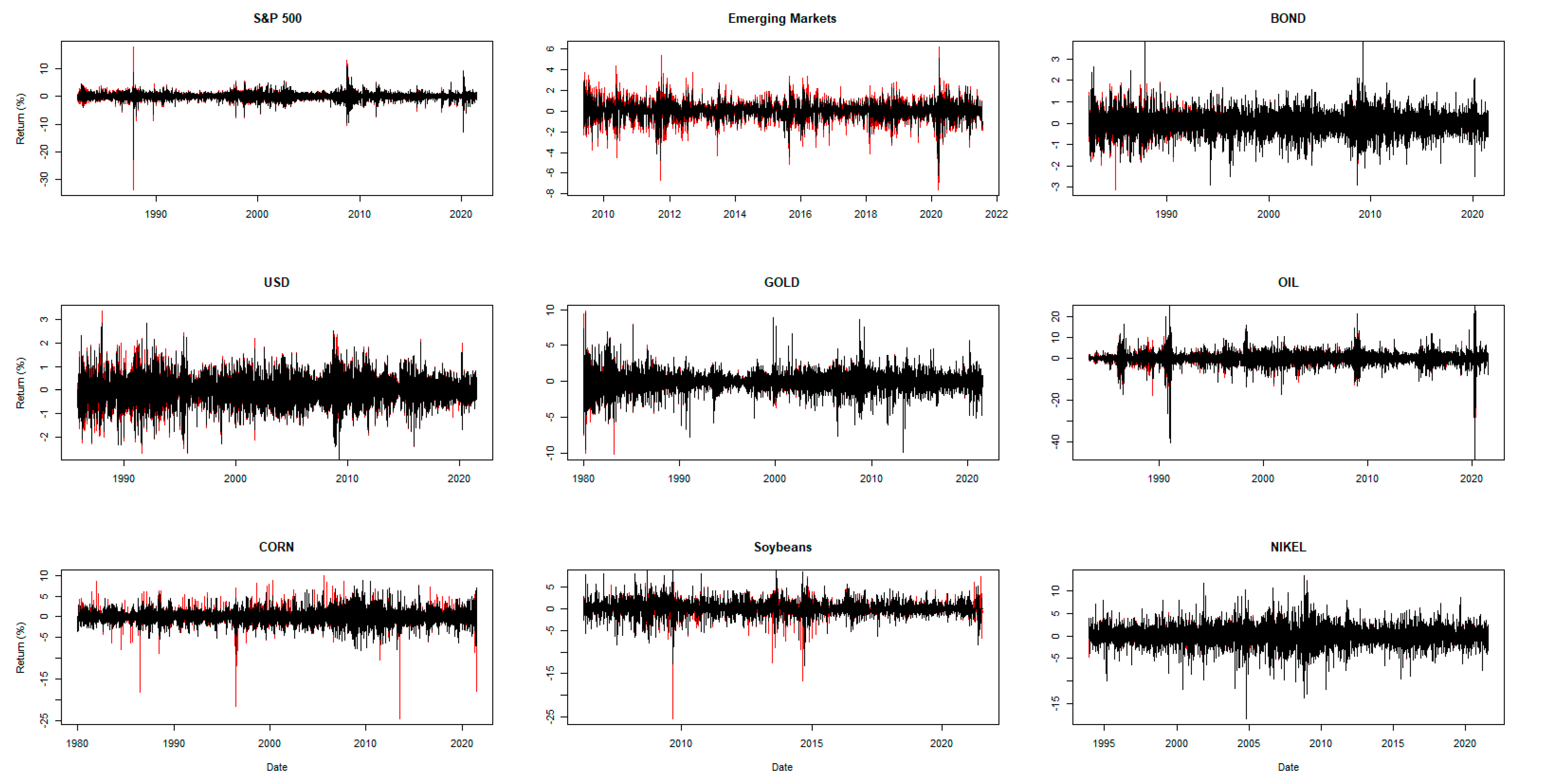
Hedging effectiveness is evaluated for a wide range of assets, including both developed and developing equity markets (S&P 500 index, MSCI Emerging Markets index), the US 10-year government bond index, the currency (US dollar index4), and various commodities (S&P gold spot price index, WTI crude oil mid-price, S&P corn spot price index, and soybean and nickel price indices in US dollars). The futures contracts employed for hedging instruments are continuous settlement price indices available from DataStream5. The data range from 1980 to 2020, although some assets have different starting values due to data availability, covering the periods of a number of economic and financial crises. Descriptive statistics for the spot and futures’ log-returns of each asset are presented in panel A of Table 1. The mean and variance properties of the return series are typical of financial returns. The Lagrange multiplier test for the ARCH effect indicates the presence of conditional heteroskedasticity, which justifies the use of a dynamic strategy to reduce the price risk exposure in the spot market, such as the rolling OLS and DCC-GARCH models. The Jarque–Bera test for non-normality indicates the existence of non-normal returns. Panel B of Table 2 shows that the estimated OLS residuals in Equation (4) are non-normally distributed, serially correlated, and heteroskedastic at the 1% significance level for the entire period of study. The strong evidence of heteroskedasticity and non-normality justifies the use of the wild bootstrap. For all assets, the Pearson correlations among the spot and futures returns indicate a strong linear association. In untabulated results, we find that the spot and futures of all included assets are co-integrated using the Johansen’s testing procedure (Johansen 1991). Figure 1 presents the time plots of the return of the different financial assets and their futures. The futures price indices appear to be more sensitive and volatile relative to changes in the spot price indices. The price reaction in most of the futures markets, except for nickel, is stronger than in the spot market, as shown by the sharper spikes in the return plots. This suggests that an incoherent strategy involving futures transactions may result in higher risks than expected.

Table 1.
Panel A—Descriptive statistics for the asset returns.
Table 2.
Panel B—Normality test, autocorrelation, and heteroskedasticity tests for residuals.
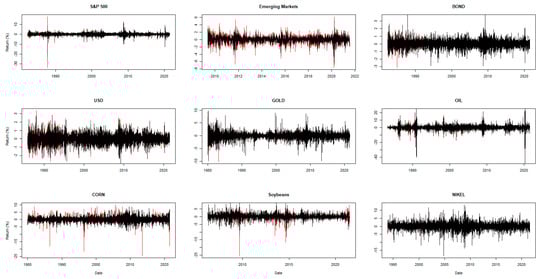
Figure 1.
Spot and futures return plots. Note: Continuous changes in the spot and futures markets are demonstrated in black and red, respectively.
5. Empirical Results
5.1. Optimal Hedge Ratio Estimates
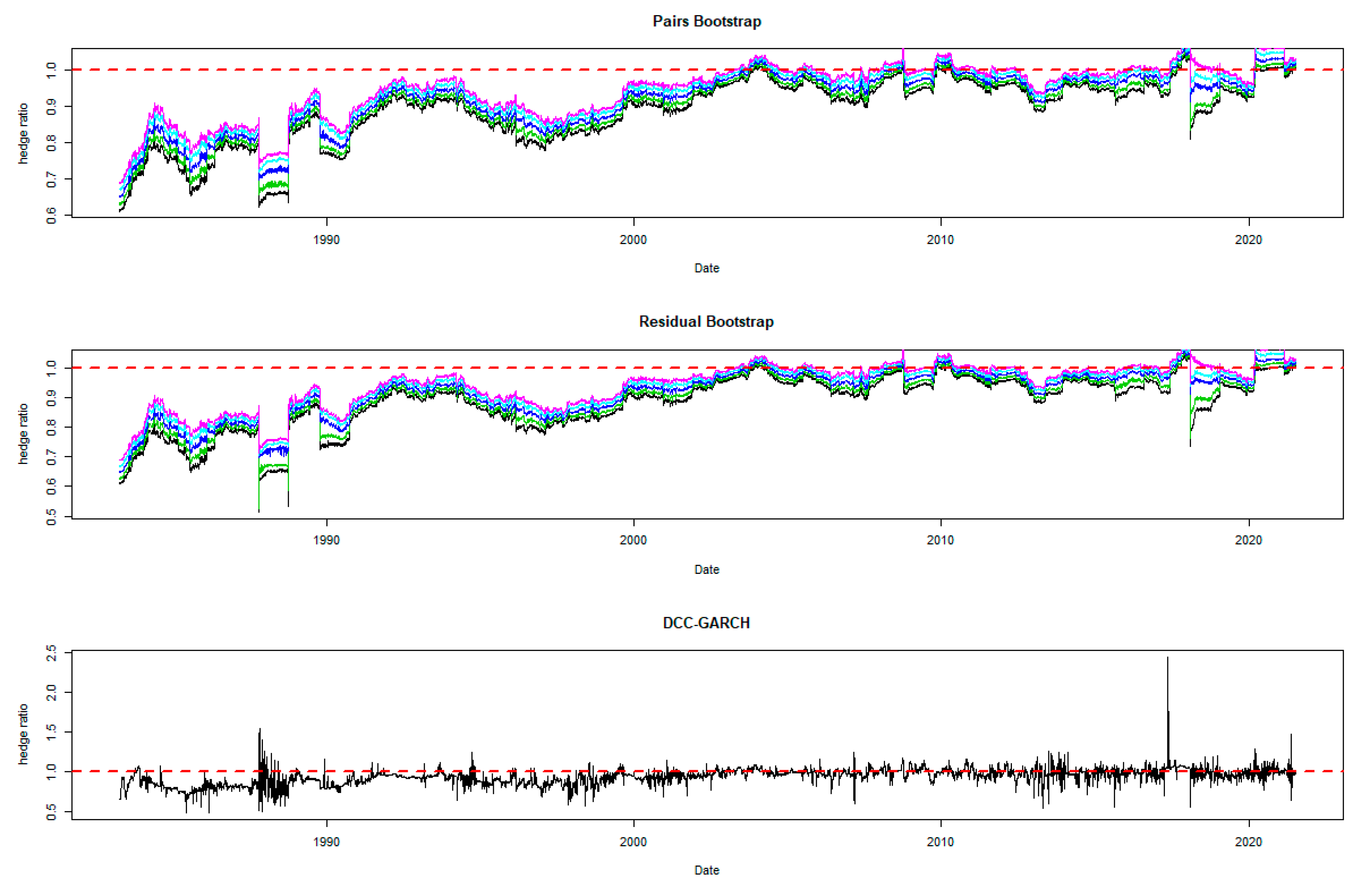
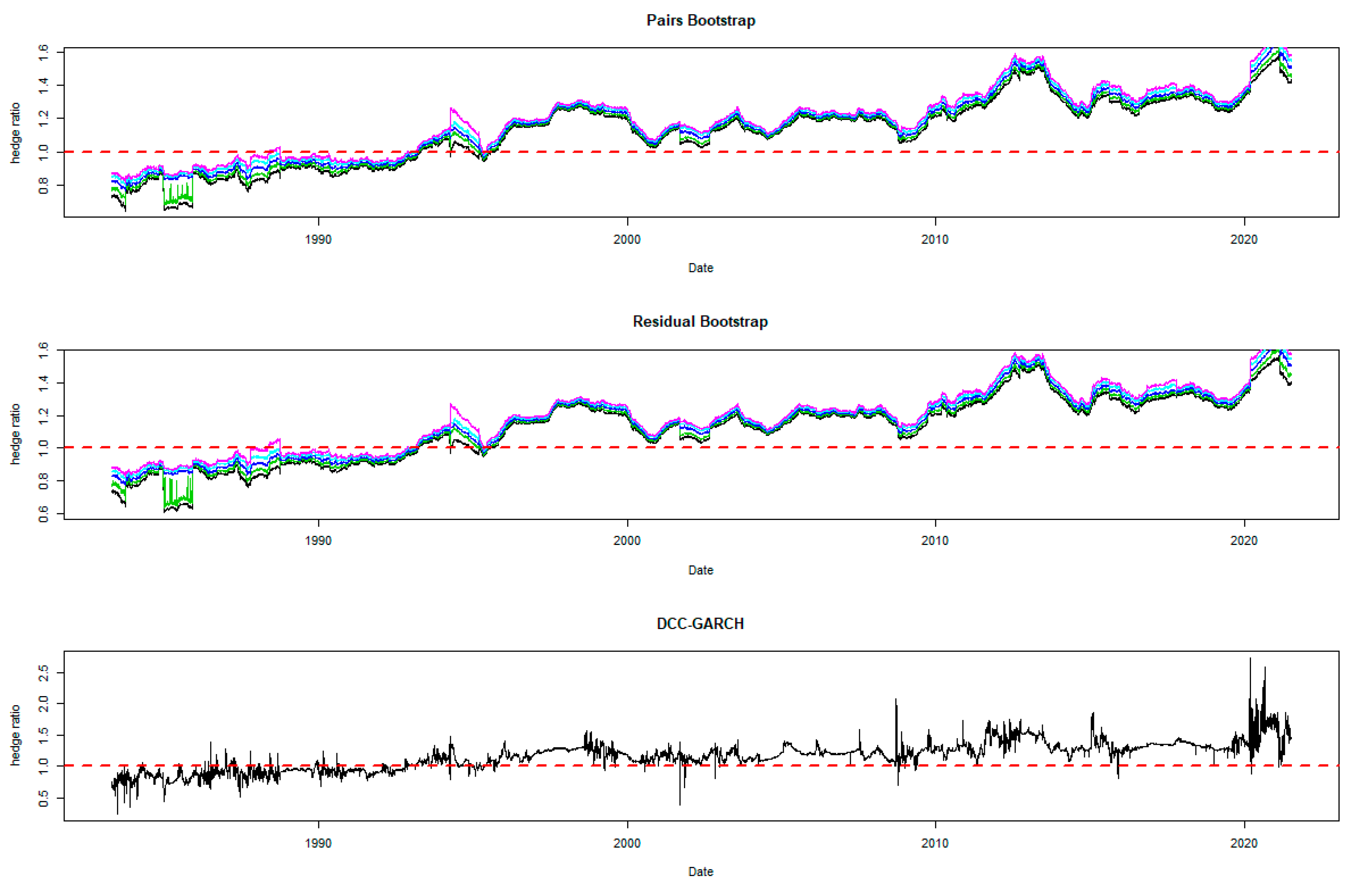
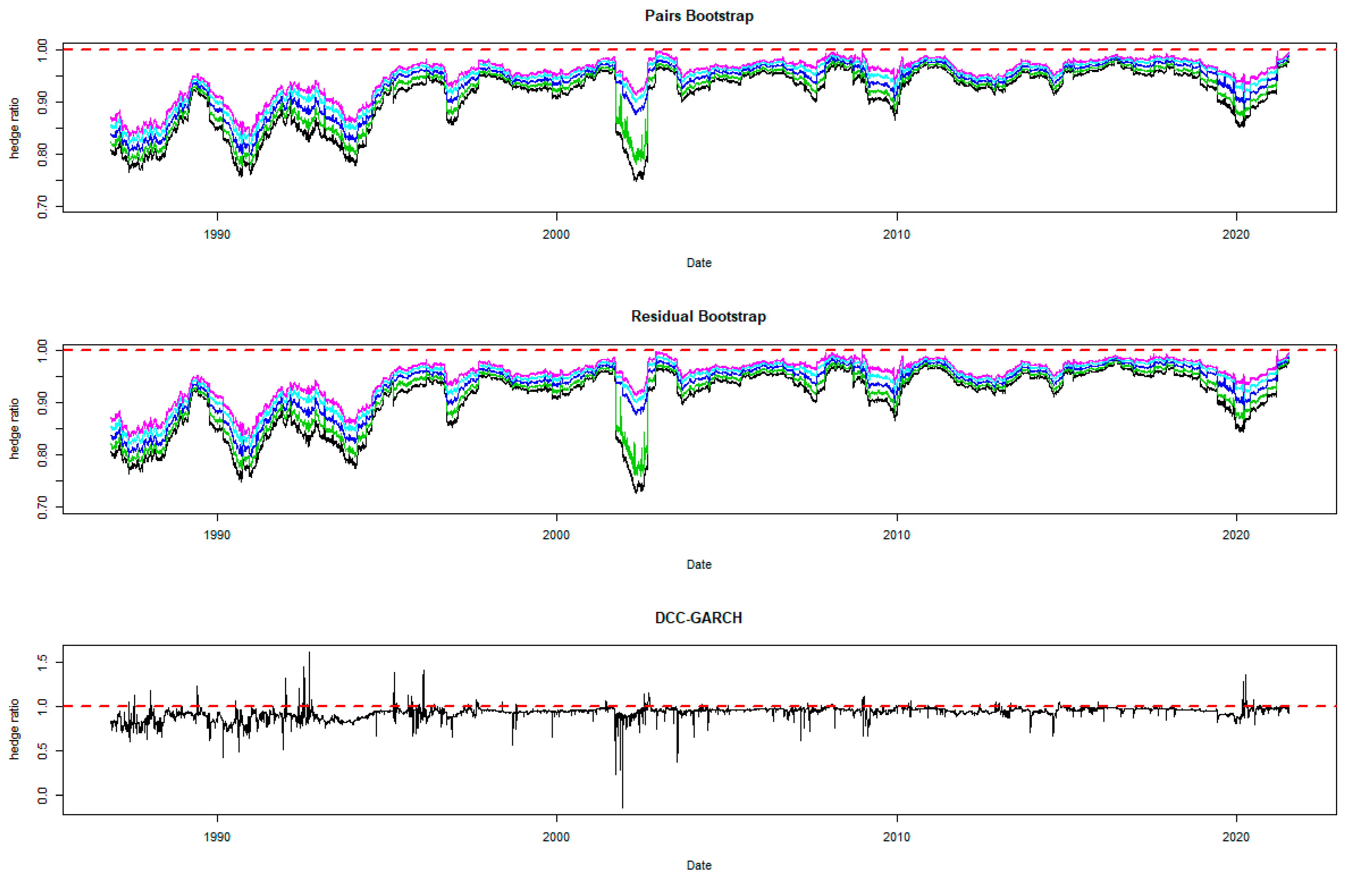
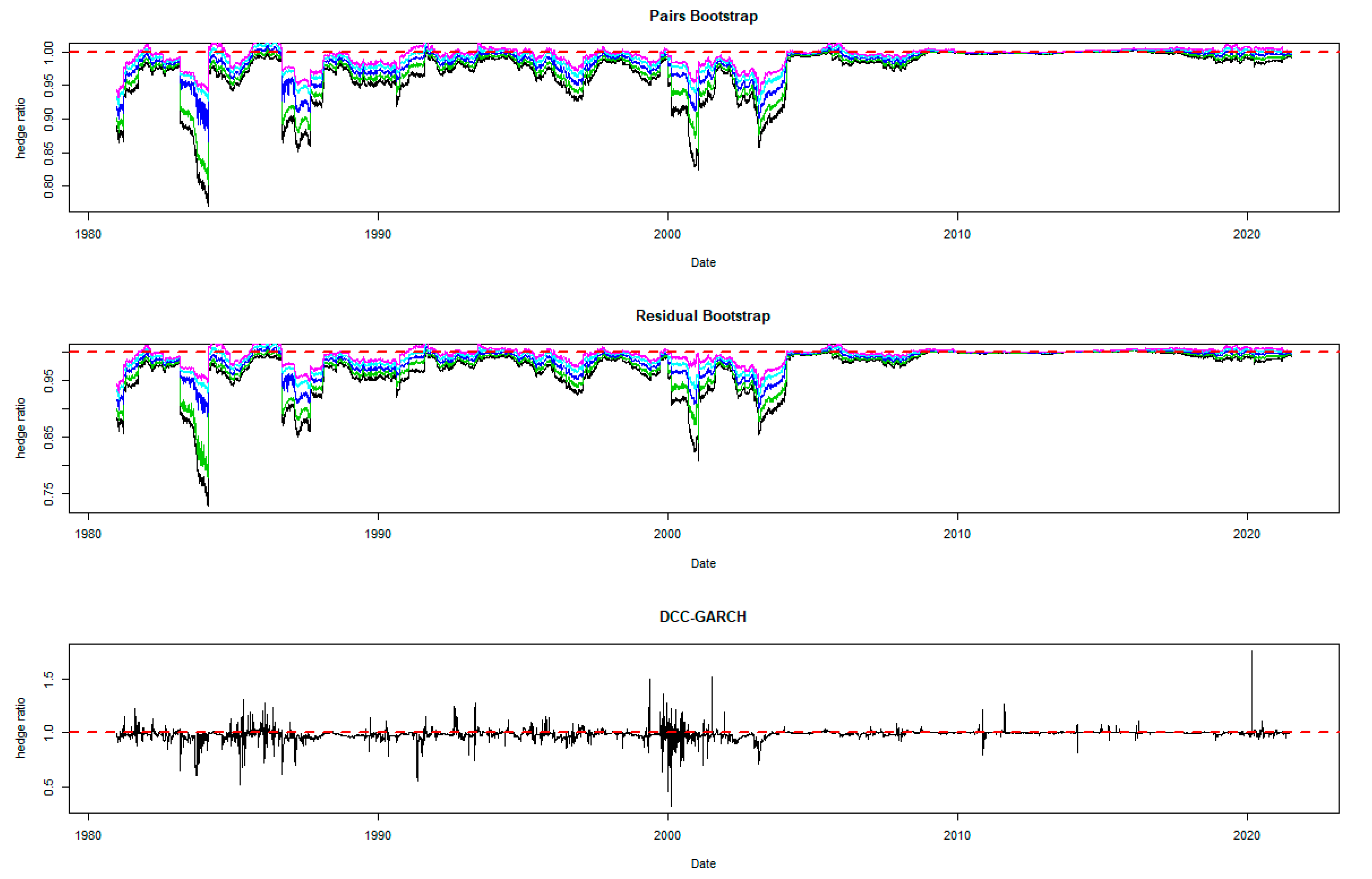
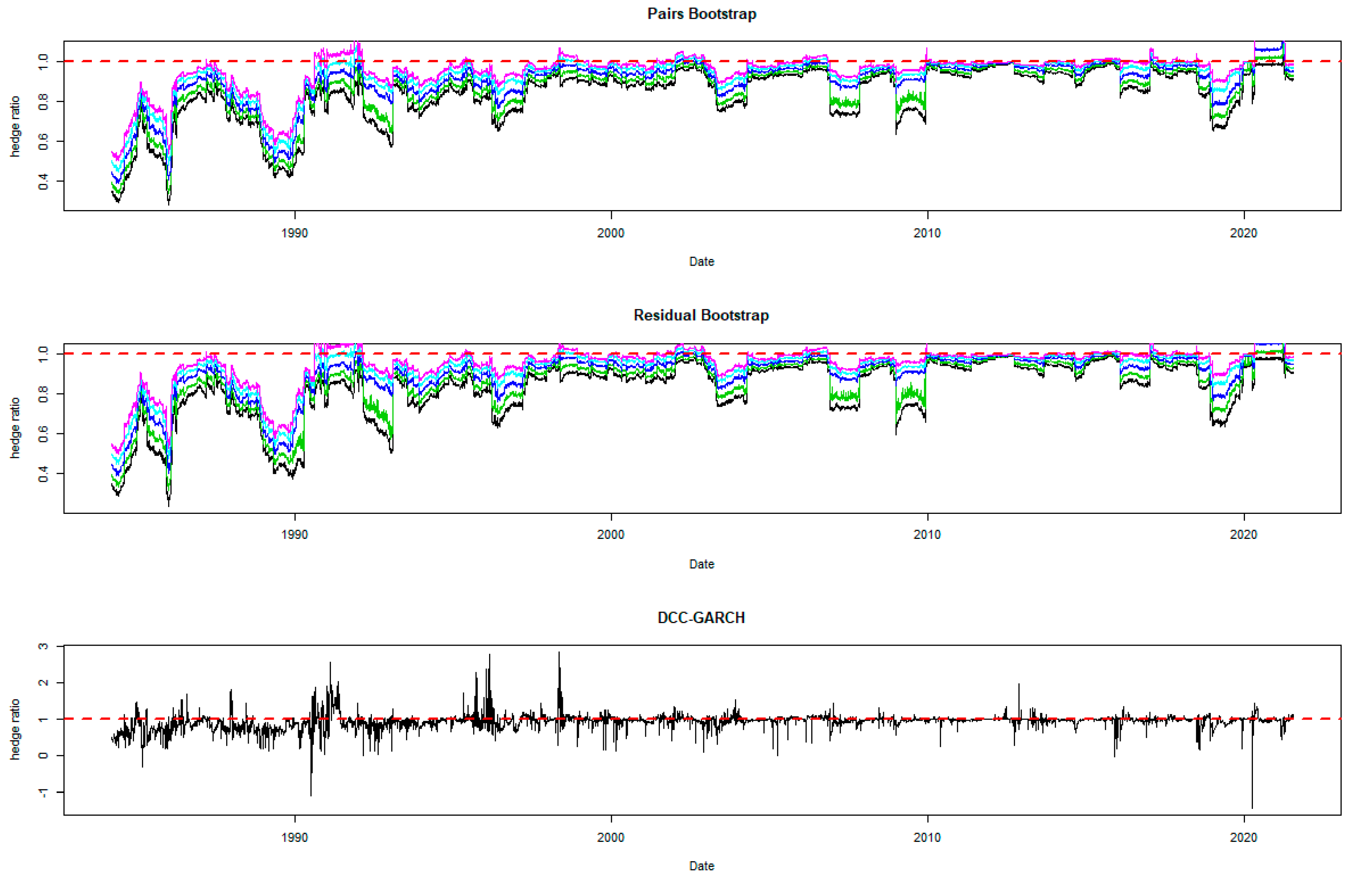
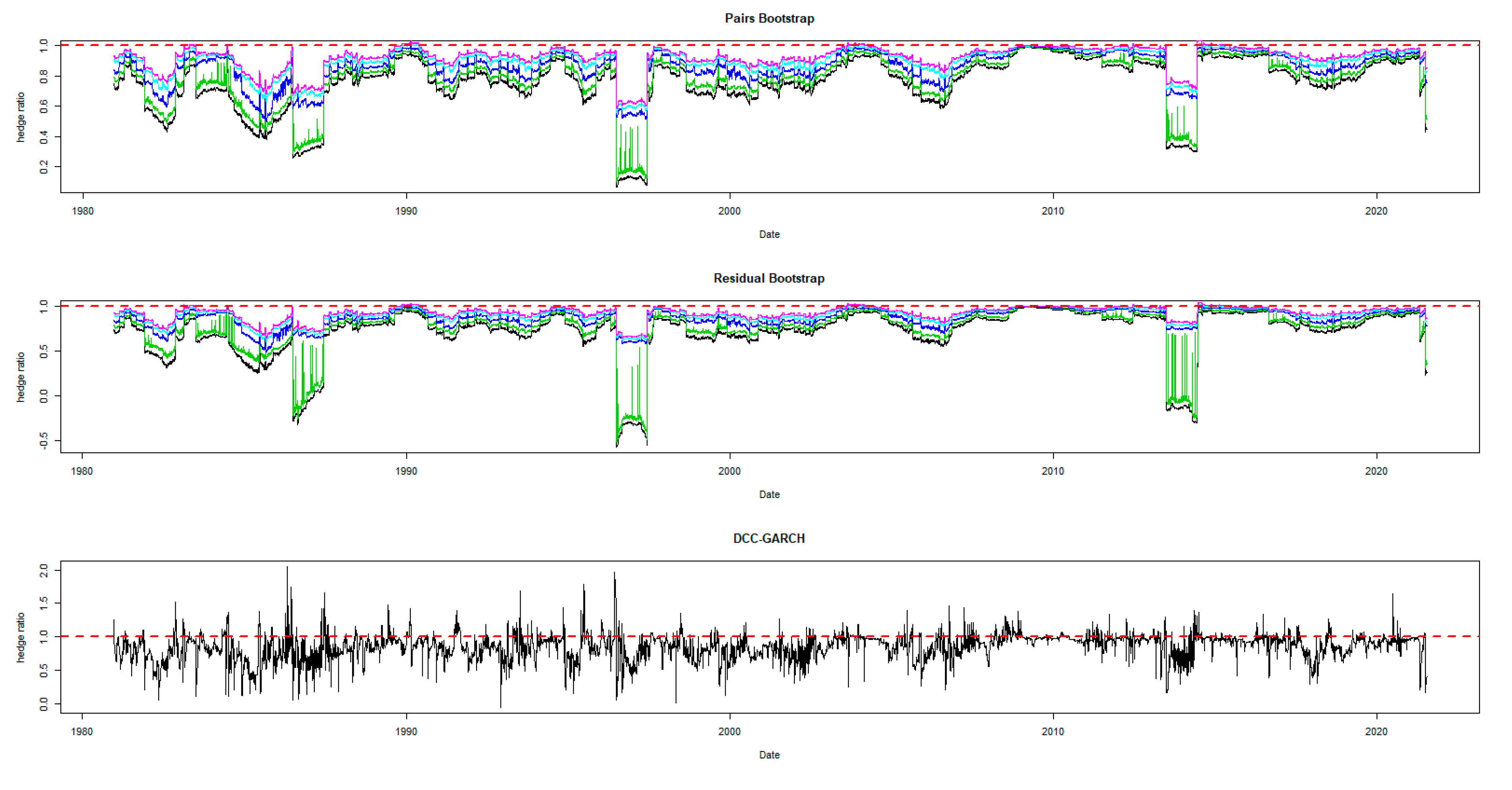
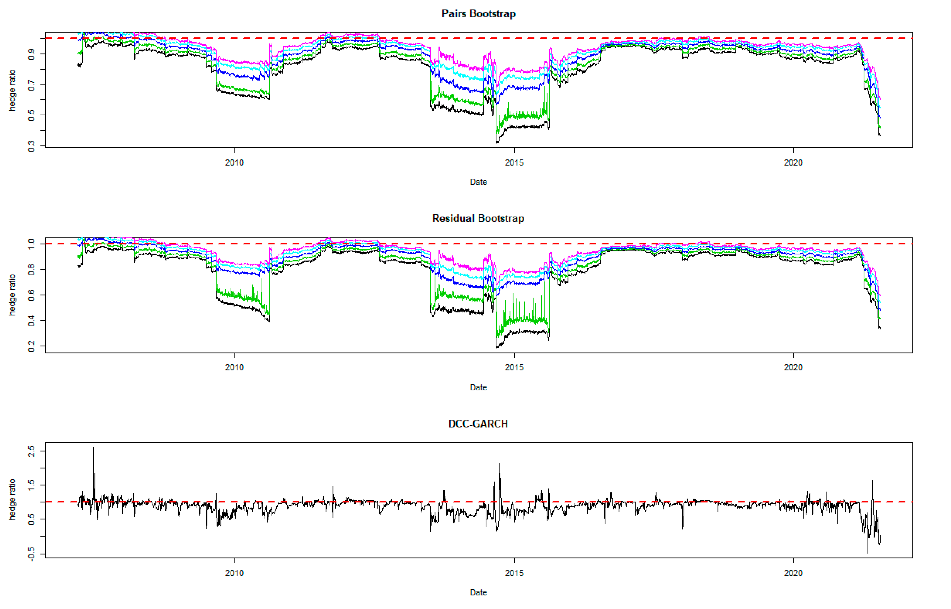
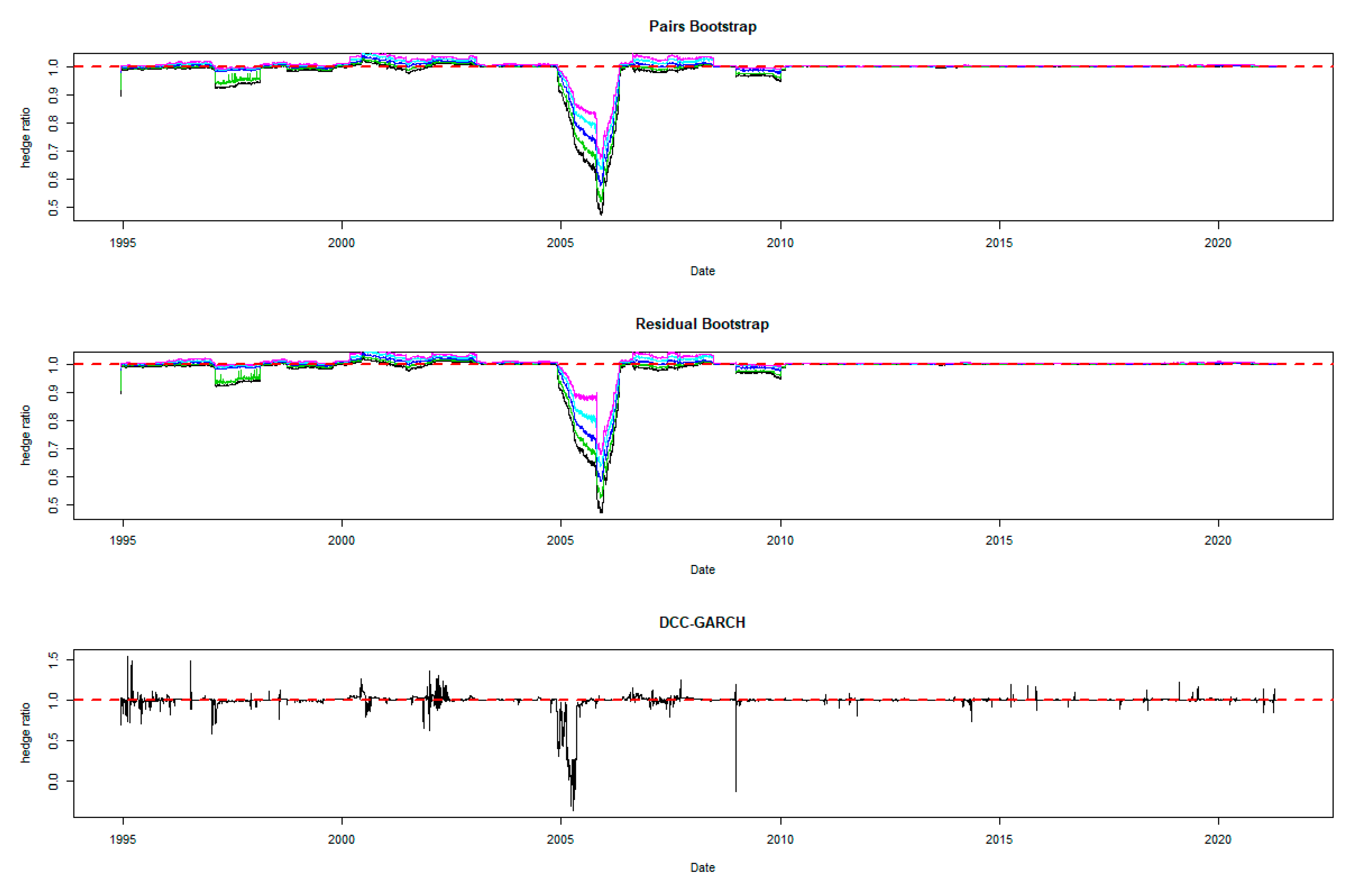
The time-varying MVHRs are shown in Figure 2, Figure 3, Figure 4, Figure 5, Figure 6, Figure 7, Figure 8, Figure 9 and Figure 10 for the included assets6. These MVHRs are generated using a moving sub-sample window of a 1-year trading period. In each figure, the bootstrap percentile-based MVHRs, using the pairs bootstrap, are reported in the top panel, while those based on the residual resampling procedure appear in the middle panel. These plots present the 95% confidence interval band within which are used for percentile-based hedging strategies. The DCC-GARCH-based MVHRs are presented in the bottom panel of the figures. As a conventional hedge, the naïve strategy is also indicated by the horizontal line at a hedge ratio of 1 in each panel for comparison.
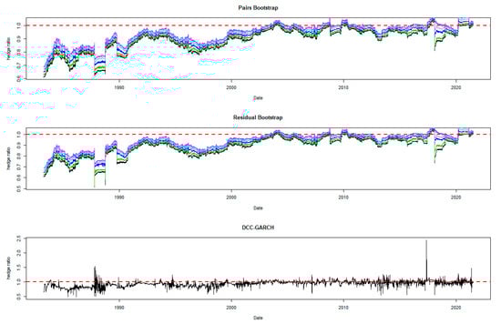
Figure 2.
Optimal hedge ratios for S&P 500 index: one-year period rolling sub-sample window.
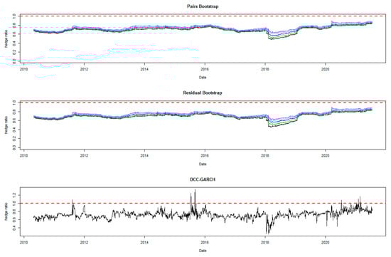
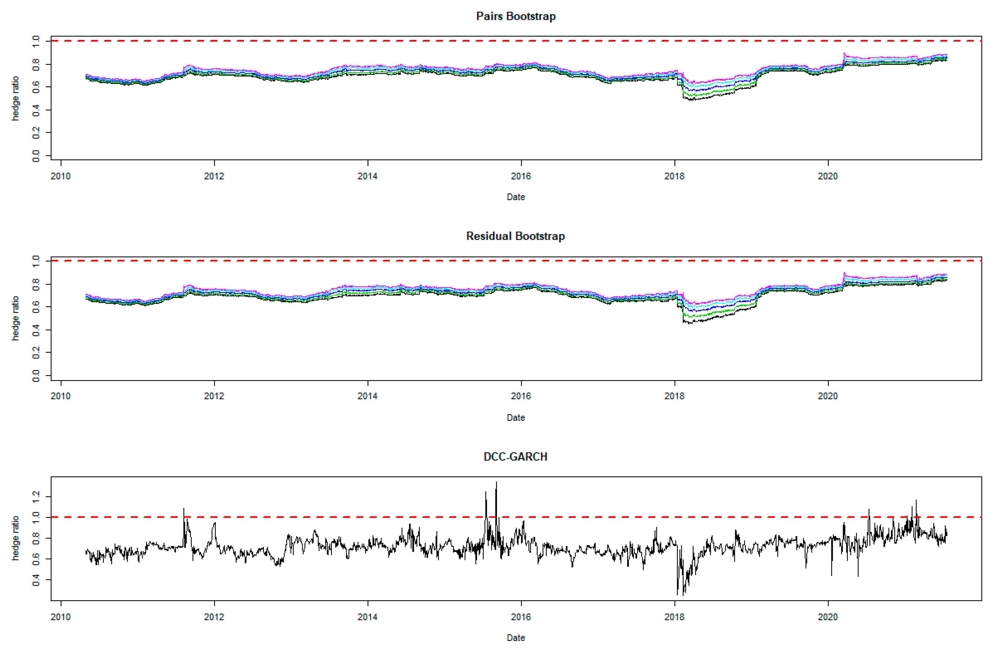
Figure 3.
Hedge ratio plots for Emerging Markets index: one-year period rolling sub-sample window. Note: The plots for bootstrap present the 95% confidence band for the optimal hedge ratio. The red horizontal line indicates the hedge ratio of 1.
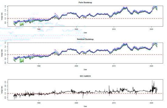
Figure 4.
Hedge ratio plots for BOND: one-year period rolling sub-sample window.
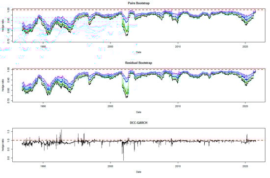
Figure 5.
Hedge ratio plots for the US dollar index: one-year period rolling sub-sample window. Note: The plots for bootstrap present the 95% confidence band for the optimal hedge ratio. The red horizontal line indicates the hedge ratio of 1.

Figure 6.
Hedge ratio plots for GOLD: one-year period rolling sub-sample window.
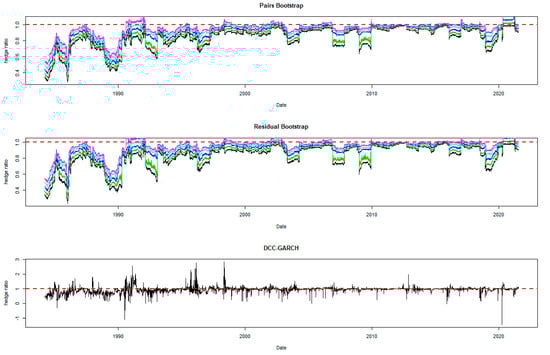
Figure 7.
Hedge ratio plots for OIL: one-year period rolling sub-sample window. Note: The plots for bootstrap present the 95% confidence band for the optimal hedge ratio. The red horizontal line indicates the hedge ratio of 1.
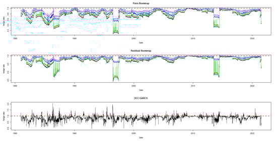
Figure 8.
Hedge ratio plots for CORN: one-year period rolling sub-sample window.
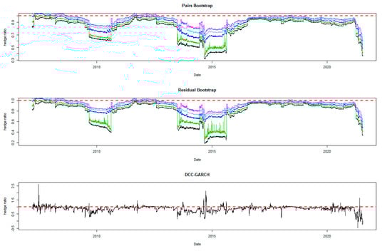
Figure 9.
Hedge ratio plots for SOYBEAN: one-year period rolling sub-sample window. Note: The plots for bootstrap present the 95% confidence band for the optimal hedge ratio. The red horizontal line indicates the hedge ratio of 1.
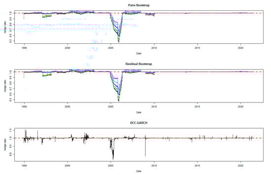
Figure 10.
Hedge ratio plots for NICKEL: one-year period rolling sub-sample window. Note: The plots for bootstrap present the 95% confidence band for the optimal hedge ratio. The red horizontal line indicates the hedge ratio of 1.
A noticeable feature in the figures is the stability of the bootstrap percentile-based MVHRs, in comparison with the DCC-GARCH counterparts. The latter are considerably more volatile, especially during the turbulent economic and financial market periods. Obviously, significant swings are observed in the time-varying DCC-GARCH-based MVHRs across the assets. The high volatility of the MVHRs based on the DCC-GARCH is also documented in previous studies (Park and Jei 2010; Chang et al. 2013; Caporin et al. 2014). From the figures, it is worth noting that changes in the MVHR using the DCC-GARCH strategy are well outside the bootstrap confidence bands. The bootstrap percentile-based MVHRs are stable, mostly well above 0 and less than 1, except for the Bond security. In contrast, the DCC-GARCH hedge ratios move erratically and are sometimes negative and even greater than 2. The observed large volatility of the DCC-GARCH-based MVHRs is probably due to the highly parametric nature and the assumed persistence effect of past shocks of the GARCH model.
Another advantage of presenting the 95% wild bootstrap confidence band is that the hedger can conduct a test for statistical significance (see Kim and Robinson 2019). For example, if the confidence band does not cover the value of 1, we cannot accept the null hypothesis that the MVHR is equal to one, at the 5% level of significance. This suggests that the MVHR is statistically different from the naïve hedge ratio. Our empirical results show that, for most of the assets, the MVHR is statistically different from 1 frequently over time at the 5% level of significance. For the US dollar and the Emerging Markets indexes, the naïve strategy has never been optimal over the entire study period at the 5% level of significance, since the 95% wild bootstrap confidence bands do not cover 1. However, the wild bootstrap confidence bands of the MVHR for gold and nickel have become tighter and increasingly convergent to 1 after 2010. The two alternative bootstrap confidence intervals appear to show a similar pattern over time, but the one based on the pairs bootstrap is slightly more stable overall. Comparing the width of the bootstrap confidence band, the time-varying degree of uncertainty associated can be assessed. A wider band indicates a higher degree of uncertainty in estimation. It is likely that the width changes depending on the prevailing market conditions that drive the degree of risk. We observe tighter confidence interval bands of MVHRs for the financial assets such as equities and bonds than the commodities (excluding nickel) and the US dollar. Particularly, the confidence interval plots of the MVHRs for gold, oil, corn and soybean show a high degree of estimation risk. This may be explained by more complicated fundamentals affecting most of the commodities’ spot and futures markets (Wu et al. 2011), especially the global supply and demand (Ai et al. 2006; Groen and Pesenti 2010; Gorton et al. 2013), effects of US dollar strength (Akram 2009), speculative activities (Park and Shi 2017), and active positions of hedge funds in both commodity and equity futures markets (Gorton et al. 2013; Büyükşahin and Robe 2014).
High degrees of estimation uncertainty of the MVHR for most of the included assets obviously appear in some common periods: 1987–1988 (effect of Black Monday), 1992–1993 (European Currency crisis), 1997–1998 (Asian Financial crisis), 2001–2003 (Dot-com bubble which triggered a sharp fall in the US dollar index), 2007–2010 (the US Subprime Housing crisis and the subsequent Global Financial crisis), and the recent health-induced crisis during 2019–2020. These turbulent episodes have influenced not only the US market but also impacted the global financial markets. However, gold appears to be an exception among the analyzed asset classes, and especially during and after the crisis starting in 2007. This may represent the popularity of gold as a safe haven asset, as discussed and investigated by Nguyen and Liu (2017).
5.2. Comparing the Hedging Effectiveness and the Robustness Checks
A hedged portfolio is constructed by taking a combined position in spot and futures returns of an asset in order to minimize the exposed risk in the physical market, using the MVHRs obtained from the alternative methods. The hedged returns in percentage are calculated daily.
We refer to the values of SV, HE, IQ, and the 95% range in Table 3 to infer downside risk, variance reduction and the variability in the hedged returns across the included assets. We first compare the hedging effectiveness between the bootstrap percentile-based methods with the naïve strategy. The bootstrap percentile-based strategies outperform the naïve hedge for most of the assets, excluding gold, oil, and nickel where similar hedging effectiveness are found. Noticeably, the naïve strategy performs worst for hedging the Emerging Markets risk. Overall, the variance reduction associated with the naïve hedge is around 1–12% lower than that for the wild bootstrap percentile-based hedge across the asset markets.
Table 3.
Statistics for the hedged portfolio returns and hedging effectiveness.
We proceed to comparing the hedging performance between the wild bootstrap approach and the DCC-GARCH model. The bootstrap percentile-based strategies show better hedging effectiveness in terms of higher variance reduction and lower downside risk for the S&P 500, Emerging Markets, oil, soybeans, and corn. The DCC-GARCH strategy shows the worst performance for hedging the oil price risk but appear to be a better model for hedging the price risk of nickel. Compared to the DCC-GARCH model, the bootstrap percentile-based strategies provide around 0.5–5% higher variance reduction with lower downside risks indicated by SV across the assets.
In general, the bootstrap percentile-based hedge ratios, especially at the 25th, 50th, and 75th percentiles of the bootstrap distribution7, which may be regarded as the defensive, neutral, and aggressive strategies, respectively, provide better hedging effectiveness. As for the point estimator, the 50th percentile (the median of the bootstrap distribution) may be preferred to the OLS-based optimal hedge ratio, since it is not influenced by extreme observations or outliers. Furthermore, the variance reduction in the hedged portfolio returns using the pairs bootstrap method is marginally higher than the residual bootstrap method, especially for corn.
To check the robustness of the superior performance of the wild bootstrap methods, we employ the statistical tests of SD as described in Section 3 for all pairs of the hedging strategies and across the asset markets. Particularly, we test for both first-order and second-order dominance relationships. We desire to test which of the hedging strategies yield a return distribution with larger benefit and lower risk. Table 4 summarizes the outcomes of the SD tests. We find statistical evidence of stochastic dominance for S&P 500 and Emerging Markets hedges but inconclusive results for the other assets. This means the alternative hedging approaches yield similar benefits with overlapping risk–return distributions, and thus the naïve strategy is still plausible given its simplicity and stability (Wang et al. 2015). However, we find that the wild bootstrap methods are second-order dominant over the naïve strategy for the included equity markets. Particularly, at least there is one percentile in the bootstrap confidence interval of the MVHR having a lower tail risk of the hedge distribution for the S&P 500 and Emerging Markets indices compared to the naïve. On the other hand, we find stochastic dominance of the bootstrap percentile-based hedging over the DCC-GARCH model only for the S&P 500 index at the 10th and 25th percentiles. Similarly, the wild bootstrap methods appear to provide a safer hedge with lower left-tail risk in hedged returns than the DCC-GARCH model.
Table 4.
Statistical dominance test of the hedged return distributions among the hedging strategies.
To further check the sensitivity of our findings to the data quality and the estimation windows, the rolling window is reduced to the 6-month period and then increased to the 2-year period. We repeat our estimation and testing procedures and our findings generally hold. When the information is reduced for the model estimation, the wild bootstrap methods are still stochastically second-order dominant over the DCC-GARCH model for the two equity markets, indicating a lower risk of big losses. However, the bootstrap approach’s superiority over the naïve strategy does hold for the case of hedging the Emerging Markets index only. When the estimation window is doubled, the dominance of our proposed bootstrap approach still holds in hedging both equity indices. Compared to the wild bootstrap hedging strategy based on resampling the residuals of the regression model, it is noted that the one based on resampling the pairs of observations provides a safer hedged return distribution with lower left-tail risk in five out of nine assets. This suggests that the endogeneity issue in the estimation of the optimal hedge ratio may play a role, since the spot and futures returns are both possibly affected by the same shocks.
6. Conclusions
The paper proposes a new method of hedging based on the percentiles of the MVHR’s bootstrap distribution. The proposed method is simple since it is OLS-based but provides a range of possible hedging strategies within the 95% confidence interval for the optimal hedge ratio. In line with Kim and Robinson (2019), it is more informative than the conventional hedging based on a single-point estimate, since the interval hedging strategy provides a hedger with a clear sense of estimation uncertainty and a range of alternative strategies, with a prescribed level of confidence. In order to estimate the percentiles of the MVHR distribution, the wild bootstrap (the one based on residual resampling and the other based on pairs resampling) is employed. This method is non-parametric for approximating the sampling distribution of a statistic based on repeated data resampling. The wild bootstrap percentiles exhibit a range of desirable features: firstly, being robust to influential outliers; and secondly, robust to non-normality and unknown forms of heteroskedasticity8. These hedging strategies are then compared to those based on the naïve method and the DCC-GARCH model with an asymmetric specification, adopting 250-day rolling sub-sample windows.
Hedging effectiveness among the alternative approaches is evaluated for a range of assets using the daily spot and futures prices from 1980. The estimation uncertainty of the MVHR is exhibited by varying width of the wild bootstrap confidence intervals during the historical turbulent periods of financial and commodity market activity. The DCC-GARCH hedge ratios are found to fluctuate in a highly volatile manner due to the specification issue, in comparison with the bootstrap percentile-based alternatives. The high volatility of the DCC-GARCH estimates adversely impact the hedging position and increase the uncertainty in hedging.
Overall, the hedging strategies based on the wild bootstrap percentiles9 are found to outperform those based on the DCC-GARCH model and the naïve hedge in terms of the hedging effectiveness, downside risk, and hedged return variability at least for hedging the equity market price risks. Our results are robust to stochastic dominance tests using bootstrap simulations and using different estimation windows. In particular, hedging strategies based on the central percentiles (the 25th, 50th, and 75th) demonstrate desirable hedging performance. The two alternative bootstrap methods perform similarly in hedging effectiveness, but the one based on resampling the pairs of observations provides a safer hedged return distribution with a lower risk of big losses. This may indicate the importance of the endogeneity issue in estimation, which is widely neglected in previous studies. While the conventional hedging methods rely solely on the point estimate of the MVHR, this paper represents the first study that proposes hedging based on the confidence interval or percentile estimation. The latter is associated with a richer information content across a range of alternative hedging strategies, which can lead to safer and more informed risk management.
Author Contributions
Methodology, P.M.N.; Investigation, J.H.K.; Writing—review & editing, D.H. and S.C. All authors have read and agreed to the published version of the manuscript.
Funding
This research received no external funding.
Institutional Review Board Statement
Not applicable.
Informed Consent Statement
Not applicable.
Data Availability Statement
Restrictions apply to the availability of these data. Data were obtained from Thomson Reuters Datastream and are available for Datastream subscribers.
Conflicts of Interest
The authors declare no conflicts of interest.
Notes
| 1 | The naïve strategy is static with a hedge ratio of 1, taking a hedging position in a futures contract equal to the exact exposure in the spot market. |
| 2 | hi is the ith diagonal element of the orthogonal projection matrix (see Long and Ervin 2000). |
| 3 | The length of the time window is constructed for rebalancing needs of a portfolio for every 12 months when the portfolio manager can revise their hedging position based on the time-varying spot–futures relationship. Choosing the time window length also facilitates the convergence issue of the rolling DCC-GARCH model. |
| 4 | The US dollar index, which has existed since 1973, is a geometrically weighted average of a basket of six currencies against the US dollar, i.e., British pound, Canadian dollar, the Euro, Japanese yen, Swedish krona, and Swiss franc. Since the US dollar is freely floated against all other foreign currencies, the Federal Reserve Bank initiated the measure of the US dollar index to provide an external bilateral trade-weighted average of the US dollar. |
| 5 | The continuous futures indices are a perpetual series of futures prices, volumes, and open interest derived from individual futures contracts. They start at the nearest contract month, which forms the first price values for the continuous series until either the contract reaches its expiry date or until the first business day of the notional contract month, whichever is sooner. At this point, prices from the next trading contract month are taken. No adjustment for price differentials is made. Thomson Reuters DataStream provides the methodology. |
| 6 | Estimation of the MVHRs based on the proposed methods is processed in R. Interested readers can find the R codes by clicking on the linked Online Appendix. |
| 7 | As suggested by an anonymous referee, interested readers and practitioners are encouraged to try different percentiles other than the ones used in this paper to find the most suitable hedging position. It is subject to underlying assets, market conditions, estimation uncertainty, confidence level, and computing resources. |
| 8 | An alternative solution to the consequential effects of the outliers or leverage points is the robust regression technique (Knez and Ready 1997; Martin and Xia 2022). However, our wild bootstrap approach is more informative and effective by estimating a confidence interval of the optimal hedge ratio for various time windows and offering a range of possible alternatives based on the estimated percentiles. |
| 9 | Maximum entropy bootstrap (“meboot”) is a powerful alternative bootstrap method to deal with endogeneity issue in the relationship between non-stationary spot and futures return data (Zanjani et al. 2021). |
References
- Ai, Chunrong, Arjun Chatrath, and Frank Song. 2006. On the comovement of commodity prices. American Journal of Agricultural Economics 88: 574–88. [Google Scholar] [CrossRef]
- Akram, Q. Farooq. 2009. Commodity prices, interest rates and the dollar. Energy Economics 31: 838–51. [Google Scholar] [CrossRef]
- Alizadeh, Amir, and Nikos Nomikos. 2004. A Markov regime switching approach for hedging stock indices. Journal of Futures Markets 24: 649–74. [Google Scholar] [CrossRef]
- Andersen, Torben G., Tim Bollerslev, Francis X. Diebold, and Ebens Heiko. 2001. The Distribution of Realized Stock Return Volatility. Journal of Financial Economics 61: 43–76. [Google Scholar]
- Barrett, Garry F., and Stephen G. Donald. 2003. Consistent tests for stochastic dominance. Econometrica 71: 71–104. [Google Scholar] [CrossRef]
- Black, Fischer. 1976. Studies of Stock Price Volatility Changes. In Proceedings of the 1976 Meetings of the American Statistical Association, Business and Economic Statistics. Washington, DC: American Statistical Association, pp. 177–81. [Google Scholar]
- Brooks, Chris, Alešs Černý, and Joelle Miffre. 2011. Optimal hedging with higher moments. Journal of Futures Markets 32: 909. [Google Scholar] [CrossRef]
- Büyükşahin, Bahattin, and Michel A. Robe. 2014. Speculators, commodities and cross-market linkages. Journal of International Money and Finance 42: 38–70. [Google Scholar] [CrossRef]
- Caporin, Massimiliano, Juan-Angel Jimenez-Martin, and Lydia Gonzalez-Serrano. 2014. Currency hedging strategies in strategic benchmarks and the global and Euro sovereign financial crises. Journal of International Financial Markets, Institutions & Money 31: 159. [Google Scholar]
- Chang, Chia-Lin, Juan-Ángel Jiménez-Martín, Esfandiar Maasoumi, and Teodosio Pérez-Amaral. 2015. A stochastic dominance approach to financial risk management strategies. Journal of Econometrics 187: 472–85. [Google Scholar] [CrossRef]
- Chang, Chia-Lin, Lydia González-Serrano, and Juan-Angel Jimenez-Martin. 2013. Currency hedging strategies using dynamic multivariate GARCH. Mathematics and Computers in Simulation 94: 164–82. [Google Scholar] [CrossRef]
- Chatfield, Chris. 1993. Calculating interval forecasts. Journal of Business & Economic Statistics 11: 121–35. [Google Scholar]
- Chen, Chao-Chun, and Wen-Jen Tsay. 2011. A Markov regime-switching ARMA approach for hedging stock indices. Journal of Futures Markets 31: 165–91. [Google Scholar] [CrossRef]
- Chen, Rongda, Bo Wei, Chenglu Jin, and Jia Liu. 2021. Returns and volatilities of energy futures markets: Roles of speculative and hedging sentiments. International Review of Financial Analysis 76: 101748. [Google Scholar] [CrossRef]
- Chen, Sheng-Syan, Cheng-few Lee, and Keshab Shrestha. 2003. Futures hedge ratios: A review. Quarterly Review of Economics and Finance 43: 433–65. [Google Scholar] [CrossRef]
- Chen, Yi-Ting, Keng-Yu Ho, and Larry Y. Tzeng. 2014. Riskiness-minimizing spot-futures hedge ratio. Journal of Banking & Finance 40: 154–64. [Google Scholar] [CrossRef]
- Christie, Andrew A. 1982. The stochastic behavior of common stock variances: Value, leverage and interest rate effects. Journal of Financial Economics 10: 407–432. [Google Scholar] [CrossRef]
- Cribari-Neto, Francisco, and Maria da Glória A. Lima. 2009. Heteroskedasticity-consistent interval estimators. Journal of Statistical Computation and Simulation 79: 787–803. [Google Scholar] [CrossRef]
- Cribari-Neto, Francisco, Tatiene C. Souza, and Klaus L. P. Vasconcellos. 2007. Inference Under Heteroskedasticity and Leveraged Data. Communications in Statistics—Theory and Methods 36: 1877–88. [Google Scholar] [CrossRef]
- Davidson, Russell, and Emmanuel Flachaire. 2008. The wild bootstrap, tamed at last. Journal of Econometrics 146: 162–69. [Google Scholar] [CrossRef]
- Ederington, Louis H. 1979. The hedging performance of the new futures markets. Journal of Finance 34: 157–70. [Google Scholar] [CrossRef]
- Efron, Bradley. 1979. Bootstrap Methods: Another Look at the Jackknife. The Annals of Statistics 7: 1–26. [Google Scholar] [CrossRef]
- Engle, Robert. 2002. Dynamic conditional correlation: A simple class of multivariate generalized autoregressive conditional heteroskedasticity models. Journal of Business & Economic Statistics 20: 339–50. [Google Scholar]
- Flachaire, Emmanuel. 2005. Bootstrapping heteroskedastic regression models: Wild bootstrap vs. pairs bootstrap. Computational Statistics & Data Analysis 49: 361–76. [Google Scholar]
- Glosten, Lawrence R., Ravi Jagannathan, and David E. Runkle. 1993. On the relation between the expected value and the volatility of the nominal excess return on stocks. The Journal of Finance 48: 1779–801. [Google Scholar] [CrossRef]
- Gorton, Gary B., Fumio Hayashi, and K. Geert Rouwenhorst. 2013. The fundamentals of commodity futures returns. Review of Finance 17: 35–105. [Google Scholar] [CrossRef]
- Groen, Jan J., and Paolo A. Pesenti. 2010. Commodity prices, commodity currencies, and global economic developments. In Commodity Prices and Markets. Chicago: University of Chicago Press. [Google Scholar]
- Hsu, Chih-Chiang, Chih-Ping Tseng, and Yaw-Huei Wang. 2008. Dynamic hedging with futures: A copula-based GARCH model. Journal of Futures Markets 28: 1095–116. [Google Scholar] [CrossRef]
- Johansen, Soren. 1991. Estimation and Hypothesis Testing of Cointegration Vectors in Gaussian Vector Autoregressive Models. Econometrica 59: 1551–80. [Google Scholar] [CrossRef]
- Kim, Jae H. 2006. Wild bootstrapping variance ratio tests. Economics Letters 92: 38–43. [Google Scholar] [CrossRef]
- Kim, Jae H., and Andrew P. Robinson. 2019. Interval-based hypothesis testing and its applications to economics and finance. Econometrics 7: 21. [Google Scholar] [CrossRef]
- Knez, Peter J., and Mark J. Ready. 1997. On the robustness of size and book-to-market in cross-sectional regressions. The Journal of Finance 52: 1355–82. [Google Scholar]
- Kroner, Kenneth F., and Jahangir Sultan. 1993. Time-Varying Distributions and Dynamic Hedging with Foreign Currency Futures. Journal of Financial and Quantitative Analysis 28: 535–51. [Google Scholar] [CrossRef]
- Ku, Yuan-Hung Hsu, Ho-Chyuan Chen, and Kuang-hua Chen. 2007. On the application of the dynamic conditional correlation model in estimating optimal time-varying hedge ratios. Applied Economics Letters 14: 503–9. [Google Scholar] [CrossRef]
- Lee, Hsiang-Tai. 2009. A copula-based regime-switching GARCH model for optimal futures hedging. Journal of Futures Markets 29: 946–72. [Google Scholar] [CrossRef]
- Lee, Hsiang-Tai. 2010. Regime switching correlation hedging. Journal of Banking & Finance 34: 2728–41. [Google Scholar] [CrossRef]
- Lee, Hsiang-Tai, and Jonathan K. Yoder. 2011. A bivariate Markov regime switching GARCH approach to estimate time varying minimum variance hedge ratios. Applied Economics 39: 1253–65. [Google Scholar] [CrossRef]
- Li, Ming-Yuan Leon. 2010. Dynamic hedge ratio for stock index futures: Application of threshold VECM. Applied Economics 42: 1403–17. [Google Scholar] [CrossRef]
- Lien, Donald. 2009. A note on the hedging effectiveness of GARCH models. International Review of Economics & Finance 18: 110–12. [Google Scholar] [CrossRef]
- Lien, Donald, and Keshab Shrestha. 2008. Hedging effectiveness comparisons: A note. International Review of Economics & Finance 17: 391–96. [Google Scholar] [CrossRef]
- Lien, Donald, Keshab Shrestha, and Jing Wu. 2016. Quantile estimation of optimal hedge ratio. Journal of Futures Markets 36: 194–214. [Google Scholar] [CrossRef]
- Lien, Donald, Yiu Kuen Tse, and Albert K. C. Tsui. 2002. Evaluating the hedging performance of the constant-correlation GARCH model. Applied Financial Economics 12: 791–98. [Google Scholar] [CrossRef]
- Liu, Regina Y. 1988. Bootstrap Procedures under some Non-I.I.D. Models. The Annals of Statistics 16: 1696–708. [Google Scholar] [CrossRef]
- Liu, Wei-han. 2016. A re-examination of maturity effect of energy futures price from the perspective of stochastic volatility. Energy Economic 56: 351–62. [Google Scholar] [CrossRef]
- Long, J. Scott, and Laurieh Ervin. 2000. Using Heteroscedasticity Consistent Standard Errors in the Linear Regression Model. The American Statistician 54: 217–24. [Google Scholar] [CrossRef]
- Maharaj, Elizabeth A., Imad Moosa, Jonathan Dark, and Param Silvapulle. 2008. Wavelet estimation of asymmetric hedge ratios: Does econometric sophistication boost hedging effectiveness? International Journal of Business and Economics 7: 213. [Google Scholar]
- Mammen, Enno. 1993. Bootstrap and Wild Bootstrap for High Dimensional Linear Models. The Annals of Statistics 21: 255–85. [Google Scholar] [CrossRef]
- Markopoulou, Chrysi E., Vasiliki D. Skintzi, and Apostolos-Paul N. Refenes. 2016. Realized hedge ratio: Predictability and hedging performance. International Review of Financial Analysis 45: 121–33. [Google Scholar] [CrossRef]
- Martin, R. Douglas, and Daniel Z. Xia. 2022. Efficient bias robust regression for time series factor models. Journal of Asset Management 23: 215–34. [Google Scholar] [CrossRef]
- Moosa, Imad A. 2017. Econometrics as a Con Art: Exposing the Limitations and Abuses of Econometrics. Cheltenham: Edward Elgar Publishing. [Google Scholar]
- Nguyen, Phong, and Wei-han Liu. 2017. Time-varying linkage of possible safe haven assets: A cross-market and cross-asset analysis. International Review of Finance 17: 43–76. [Google Scholar] [CrossRef]
- Park, Jin Suk, and Yukun Shi. 2017. Hedging and speculative pressures and the transition of the spot-futures relationship in energy and metal markets. International Review of Financial Analysis 54: 176–91. [Google Scholar] [CrossRef]
- Park, Sung Yong, and Sang Young Jei. 2010. Estimation and hedging effectiveness of time-varying hedge ratio: Flexible bivariate garch approaches. Journal of Futures Markets 30: 71. [Google Scholar] [CrossRef]
- Shrestha, Keshab, Ravichandran Subramaniam, Yessy Peranginangin, and Sheena Sara Suresh Philip. 2018. Quantile hedge ratio for energy markets. Energy Economics 71: 253–72. [Google Scholar] [CrossRef]
- Su, Yi-Kai, and Chun-Chou Wu. 2014. A New Range-Based Regime-Switching Dynamic Conditional Correlation Model for Minimum-Variance Hedging. Journal of Mathematical Finance 4: 207. [Google Scholar] [CrossRef]
- Tauchen, George, Harold Zhang, and Ming Liu. 1996. Volume, Volatility, and Leverage: A Dynamic Analysis. Journal of Econometrics 74: 177–208. [Google Scholar] [CrossRef]
- Waldmann, Elisabeth. 2018. Quantile regression: A short story on how and why. Statistical Modelling 18: 203–18. [Google Scholar] [CrossRef]
- Wang, Yudong, Chongfeng Wu, and Li Yang. 2015. Hedging with futures: Does anything beat the naïve hedging strategy? Management Science 61: 2870–89. [Google Scholar] [CrossRef]
- White, Halbert. 2000. A reality check for data snooping.(Statistical Data Included). Econometrica 68: 1097. [Google Scholar] [CrossRef]
- Wu, Feng, Zhengfei Guan, and Robert J. Myers. 2011. Volatility spillover effects and cross hedging in corn and crude oil futures. The Journal of Futures Markets 31: 1052–75. [Google Scholar] [CrossRef]
- Zanjani, Zeinab, Pedro Macedo, and Isabel Soares. 2021. Investigating Carbon Emissions from Electricity Generation and GDP Nexus Using Maximum Entropy Bootstrap: Evidence from Oil-Producing Countries in the Middle East. Energies 14: 3518. [Google Scholar] [CrossRef]
Disclaimer/Publisher’s Note: The statements, opinions and data contained in all publications are solely those of the individual author(s) and contributor(s) and not of MDPI and/or the editor(s). MDPI and/or the editor(s) disclaim responsibility for any injury to people or property resulting from any ideas, methods, instructions or products referred to in the content. |
© 2024 by the authors. Licensee MDPI, Basel, Switzerland. This article is an open access article distributed under the terms and conditions of the Creative Commons Attribution (CC BY) license (https://creativecommons.org/licenses/by/4.0/).