
Are Regulatory Short Sale Data a Profitable Predictor of UK Stock Returns?


Downing College and Faculty of Economics, University of Cambridge, Cambridge CB2 1DQ, UK
J. Risk Financial Manag. 2024, 17(8), 320; https://doi.org/10.3390/jrfm17080320
Submission received: 20 June 2024
/
Revised: 18 July 2024
/
Accepted: 23 July 2024
/
Published: 25 July 2024
(This article belongs to the Special Issue Empirical Research on Asset Pricing and Portfolio Selection)
Abstract
:Regulator-required public disclosures of net short positions do not provide a profitable investment signal for UK stocks across a variety of portfolio formation methodologies. While long-short (zero initial outlay) portfolios based on this signal usually make a profit on average, it is rarely statistically significant in either gross or risk-adjusted terms. The issue is that the short sides of the portfolios make substantial losses. Unit initial outlay portfolios based on the disclosures do not generally significantly outperform the market, either. Where they do significantly outperform the market, this outperformance is economically modest.
Keywords:
short sales; short selling regulation; net short position disclosure; investment signal; anomalyJEL Classification:
G11; G141. Introduction
In November 2012, European Union (EU) Regulation 236/2012 brought into force disclosure requirements that give rise to a freely available database of all large net short positions held in stocks traded on EU markets. The database is made available to investors with only a short lag of up to a couple of days. It gives access to daily data on short holdings in specific stocks, something which has previously only been available for a fee. Conversations with practitioners indicate that these fees are high and that uptake is subsequently limited. It is therefore of practical interest to examine whether the new, freely available information on other investors’ short positions can be used profitably. I examine this question from the point of view of the UK stock market—the largest and most liquid in Europe. Considering a wide variety of portfolio formation techniques, all in all, there appears to be little profit to be gained from using this information to form portfolios.
First, I look at standard long-short portfolios, of the sort commonly used to study potential new investment signals. I consider equal-, value- and net short position-weighted long-short portfolios with zero initial outlay. These portfolios go long in stocks with a low level of total (aggregated across investors) declared net short positions and short in stocks with a high level of total declared net short positions. Since the rules exempt market making and hedging trades from notifications, the rationale is that short sellers are revealing their beliefs and private information. As short sellers are likely to be more sophisticated investors than the average investor, mimicking their positions could therefore be profitable. This has proved to be the case in previous studies using proprietary or paid-for short position information (e.g., Boehmer et al. (2008); Diether et al. (2009)). Moreover, short sale constraints can slow the impounding of negative information into the stock price, so that a rise in short selling may be predictably followed by further negative returns. Diamond and Verrecchia (1987), Hong and Stein (2003), and Miller (1977) show how short sales constraints can slow the adjustment speed to bad news when investors have heterogeneous beliefs.
While these long-short portfolios are profitable on average, only the equal-weighted portfolio has a mean gross return which is statistically significant at the 5% level. Its average risk-adjusted returns are not (statistically) significant. Scaling positions by volatility to reduce portfolio volatility does not improve the statistical significance of any profitability. The long sides of these long-short portfolios tend to make substantial gains, but the short sides tend to make substantial losses. Going beyond the standard approach of forming portfolios based on the most recent declarations does not solve this problem. I find similar results using information about the trend in short positions, which captures signal strength. Rebalancing the portfolios less frequently to make them less responsive to signal noise does not remedy the lack of long-short portfolio profitability, either. This is the case even when losses in the less frequently rebalanced portfolios are controlled with stop-loss rules. Nonetheless, consistent with Boehmer et al. (2010), I find that the long sides of the standard equal- and value-weighted long-short portfolios are highly profitable. Moreover, they produce significant risk-adjusted returns, as measured against a variety of risk factors.
I therefore construct fully invested (unit initial investment) portfolios based on the net short position disclosures too. Using portfolios of all stocks as a benchmark shows how much information is in the short disclosures, above and beyond a strategy that simply buys every stock listed on the FTSE350. When these fully invested portfolios based on declared net short positions are allowed to take short positions, they do not generally outperform portfolios of all stocks. In fact, the value-weighted versions of these fully invested portfolios underperform the value-weighted portfolio of all stocks. I also look at fully invested portfolios based on the disclosures which are long-only. Both the equal-weighted long-only portfolio based on the most recent disclosures and the long-only portfolio weighted by the strength of the trend in disclosures significantly outperform the comparable portfolios of all stocks. However, the gain is relatively modest in both cases: one percentage point per year in both gross and risk-adjusted terms.
The above results for both long-short and fully invested portfolios are robust over time, as shown by rolling window analysis. They are also robust to considering only the sub-samples of stocks where short sale data-based strategies have previously been shown to be particularly profitable (see Section 4.2.1), as well as to the various empirical choices made in portfolio formation (see Section 4).
All of the strategies discussed so far are feasible strategies. That is, they account for the lag between a position being taken, a report being made to the regulator, and the regulator publishing the report. A possible explanation for the lack of profitability of portfolios based on the short sale disclosures is that the publication lag causes the strategies to act on (slightly) stale information. However, this is not the case. When I ignore the publication lag and assume that the disclosures become available when the positions are taken, the results are largely unchanged. For the long-short portfolios, the short sides generally continue to make substantial losses. Even in the best case, the annual profit to the short side is just 0.6% per year. The fully invested portfolio returns are largely unaffected by assuming away the disclosure lag.
It may be tempting from the findings without the disclosure lag to conclude that the underlying declared short positions were not profitable, but this would be misleading. The positions are only reported once they cross a certain size threshold and so the early trades may be better timed than the hypothetical positions considered here. Moreover, the results here relate to the marginal short position, rather than the average short position. Since the strategies here must wait until an investor has a large short position in a stock before they can take a short holding themselves, it may simply be that they are taking short positions too late for them to be profitable, as the stocks can no longer profitably absorb further short interest. Indeed, evidence on actual short positions suggests they are profitable Jank and Smajlbegovic (2017); Wang et al. (2017). If it is the case that stocks can no longer profitably absorb short interest by the time the declarations are made, strategies using declared net short positions in other countries will not be profitable either.
This paper relates to a set of literature that began with studies of US short sale data. Studies of whether short sale data could be used profitably in US stock markets have been positive, at least before costs are considered. Using proprietary NYSE order data between January 2000 and April 2004, Boehmer et al. (2008) show that long-short strategies of the kind I study here can yield substantial average returns of 3.8% per month, or an annual risk-adjusted return of 16%. Given the extremely high profits, rarity of recalls, and relatively low direct costs of shorting most stocks, Boehmer et al. (2008) argue their strategies’ profitability would survive accounting for trading costs. Diether et al. (2009) use similar data for NYSE, AMEX, and Nasdaq stocks in 2005. They construct their short sale measures from SEC-required disclosure data.1 Diether et al. (2009) also find positive and significant risk-adjusted returns to short sale-based strategies. However, they note that smaller stocks are disproportionately represented in the short leg of their strategies and that the cost of shorting these is relatively high. Diether et al. (2009) therefore caution that their strategies’ profitability may not survive costs.
UK studies of strategies based on short sale data have been more mixed than those in the US, even before costs are accounted for. So far, these studies have focused on long-short strategies. Au et al. (2009) analyse equal- and value-weighted long-short portfolios which go long in stocks with low short interest and short in stocks with high short interest. Their short interest measures are based on daily subscription-access short sale data for FTSE350 constituents between September 2003 and September 2006. The equal-weighted long-short portfolio makes a statistically significant average profit, but the value-weighted portfolio’s profit is insignificant. For both the equal- and value-weighted portfolios, the short side makes a loss on average. Likewise, Andrikopoulos et al. (2012) find that profits of equal- and value-weighted long-short portfolios formed on weekly short interest are generally insignificant. Again, the short legs cost these portfolios money. Andrikopoulos et al. (2012) use a broader and longer sample of 1645 UK stocks between August 2004 and February 2012, also using subscription-access data. In keeping with Au et al. (2009) and Andrikopoulos et al. (2012), Boehmer et al. (2022) find that daily measures of short selling have no significant predictive power over cross-sectional returns looking at a panel of 894 UK stocks between July 2006 and December 2014. However, while not studying a trading strategy directly, Mohamad et al. (2013) find that the most highly shorted stocks have significantly negative returns over the 15 trading days after this information is published via a paid-for service. This suggests that a trading strategy based on this information could be profitable. They use daily data for FTSE350 stocks over the period from September 2003 to April 2010.
Unlike the databases used by Au et al. (2009), Andrikopoulos et al. (2012), and Boehmer et al. (2022), the regulatory dataset I use here excludes market making and hedging trades, which are exempt from the disclosure requirements. This gives the regulatory data the potential to contain more information than the other databases, since it is the private information of active short sellers that these strategies are trying to replicate. However, the losses to the short baskets found in Au et al. (2009) and Andrikopoulos et al. (2012) are repeated here. This finding would suggest that the informational gain from excluding market making and hedging trades is more than offset by the informational loss of using publicly available data of only large positions.
Using US data, Boehmer et al. (2010) find that the majority of the profits to a long-short strategy based on short selling activity comes from the long leg. Not only does relatively high shorting activity contain bad news for a stock’s prospects, but relatively low shorting activity contains good news, too. This finding is all the more striking since costs to going long on a stock are considerably less than the costs of taking a short position on a stock. The good news effect of little short selling has not, as far as I am aware, yet been analysed for the UK. Since such a strategy only involves long positions in stocks, it is relatively low-cost, especially when the short selling data are freely available. I analyse such long-only portfolios here. While the returns to them look high in absolute terms, the strategies do not significantly outperform portfolios of all stocks.
A key difference between this paper and those discussed so far is that I use data which are available for free, while the data used in earlier papers are paid for. The cost to using free data is that data on net short positions only become available once those positions are large. To the best of my knowledge, the only other study to use the data made available as a result of the EU short selling regulations as the basis for an investment strategy is Della Corte et al. (2022). They consider a “short conviction” strategy for 15 EU markets (including the UK) between November 2012 and December 2018. This strategy goes short in stocks with the highest weight in investors’ short baskets, as measured imperfectly by the declared positions, and long in stocks with the lowest non-zero weights in investors’ short baskets. The strategy only applies to stocks with non-zero declared short positions. This strategy produces a positive alpha of more than 8% a year, and it continues to perform strongly once transaction and borrowing costs and securities lending market frictions, such as the availability of stocks for lending and leverage constraints, are accounted for. I study a different and complementary type of strategy here—one which explicitly uses information from the fact that certain stocks do not have declared net short positions. This is closer to the standard long-short strategy typically (e.g., inter alia, by Andrikopoulos et al. 2012; Au et al. 2009; Boehmer et al. 2008; Diether et al. 2009). Doing so means I am also able to consider whether the Boehmer et al. (2010) good news in short interest result extends to the UK for declared short positions.
Other studies use the short sale disclosure data to examine how actual declared short positions have performed. Jank and Smajlbegovic (2017) do so for all EU markets (including the UK), finding that these positions have been profitable on average but not significantly so. Jones et al. (2016) treat the short sale disclosures as events and find negative cumulative abnormal returns after disclosures. These are only significant for longer event windows, although the focus is on the first disclosed short position in a stock. Urbanke (2019) uses declared short positions from 12 EU markets (including the UK) to show that short sellers are generally trend-following investors. While not studying an investment strategy directly, Urbanke (2019) also considers what would happen if investors entered their disclosed positions up to 10 days after they actually did. A cap-weighted portfolio of such “copy cat” positions has a positive but insignificant alpha.
The richness of the short sale disclosure data makes many other types of study possible as well. Geraci et al. (2023) use the declared net short position data to show that common short sellers can explain excess return correlation. Huo et al. (2023) focus on UK-listed stocks and show that short positions are more profitable when the investor is geographically closer to the issuing firm and that short positions are geographically correlated among investors. Jank et al. (2021) combine these data with private short position disclosures to examine how investors behave at the disclosure threshold.
2. Data and Methods
2.1. Net Short Position Disclosures
As of 1 November 2012, an investor in any EU-listed stock with a sufficiently large net short position must notify the national regulator. For the UK, this is the Financial Conduct Authority (FCA). I work with public notifications, which must be made once the net short position is 0.5% or greater of the issued share capital of a given company. Further notifications must be made at each 0.1% increment or decrement and a notification must also be made once the position drops below 0.5%.2 These notifications are published on the FCA’s website by the close of business on the day the notification is made. Notifications are made the trading day after the position crosses the relevant threshold.
The disclosures ought to be informative about short sellers’ private information and beliefs. Market making and liquidity providing trades are exempt from the notification rules. Moreover, net short positions are the calculated net of delta-adjusted derivative positions. A short position created to hedge a derivative position does not count towards the net total. Because market making, liquidity providing, and hedging trades are unrelated to anticipated price changes, they do not reveal a short seller’s private information. In addition, synthetic short positions—holdings of derivatives such as options that perfectly replicate the payoff of a short position—must also be reported, again on a delta-adjusted basis. Synthetic short trades can attract lower transaction costs than conventional short trades (Daske et al. (2005)). They may therefore be an important source of information about investors’ expectations of price movements. Note that the rules apply to any investor, even if they are domiciled outside the EU.
Net short position declarations required by the regulations outlined above must be made by 3.30 p.m. the trading day after the position was established/modified. The FCA publishes the public notifications by the close of business that same day. A notification triggered by a trade on day t must be made by 3.30 p.m. on and that information is published by the FCA by close of business on . However, since the FCA’s close of business is 6 p.m. and FTSE trading closes at 4.30 p.m., it is unclear whether the FCA disclosures will be available to trade on before the close of trading on , or if investors would have to wait until the market opens on . I err on the side of caution and assume that investors have to wait until the market opens at . However, assuming that investors can instead trade at the close of day makes little difference to the results (see Section 4.1).
Given the truncated nature of the data, it is necessary to make some assumptions to construct a net short position measure from the public disclosures. Note that disclosures are made by investor by stock. I assume that open positions with no new disclosures on a given day are unchanged. If there is a new declaration of a position of 0.51% of issued share capital on Monday and no new declaration on Tuesday, I assume the position remains 0.51% on Tuesday. I also assume that positions that are below the 0.5% reporting threshold are 0%. If Wednesday’s position falls to 0.49%, then I take the position to be 0% from Wednesday onwards, since no further tracking of the position is possible. This gives a daily position series for each investor for each stock. To obtain the total declared net short positions, I sum declarations across investors for each stock on each day. To evaluate the robustness of the results to these assumptions, I consider a measure of net short positions that requires no such assumptions: the number of distinct declarations of positions greater than 0.5% per stock per day. The results are robust to such a change (see Section 4.2).
The short selling measure I use here, (declared) net short position size as a percentage of share capital outstanding, corresponds most closely to the short interest ratio, the number of shares held short as a percentage of the number of shares outstanding. Short sales can also be measured by active utilisation, the percentage of shares available for loan that are held short, and share borrowing fee (e.g., as in Andrikopoulos et al. 2012). Information about the number of shares available for shorting and borrowing fees is not publicly available and therefore not used here. A further alternative would be the days-to-cover ratio (used by, e.g., Boehmer et al. 2022). It is the number of shares held short divided by average daily trading volume and is the expected number of days it would take for short sellers to cover all their positions on the open market. By dividing by volume, it includes liquidity information.
2.2. Sample and Data
My sample is the constituents of the FTSE350 index on the last date of the sample period (13 December 2018).3 These are all large and liquid stocks. I obtain the return and characteristic data needed to form and evaluate portfolios from Refinitiv Eikon. I adjust returns for dividends since short sellers must pay any dividends distributed to the stock owner, and this allows for the reinvestment of dividends on the long side—a key source of growth.
Short disclosure data are available for positions taken as of 31 October 20124, and therefore, the first position can be taken as of 2 November 2012, assuming the FCA’s public disclosures of positions on day t reach traders between market close on and market open on . The first return in the back test return series is realised on 1 November 2013, since some portfolio formation schemes use up to 252 days of net short position information in their formation. The last date in my sample is 13 December 2018. The back test return series contain 1295 observations.
2.3. Net Short Position Disclosures across the Sample
I look at disclosures for stocks in the FTSE350 index. There is a total of 30,357 disclosures (position openings, updates, and closures) across the sample period. A total of 101 stocks have no disclosures associated with them. There were 114 disclosures made when the disclosure regulations initially entered into force.5 Table 1 shows summary statistics relating to the disclosures from the day after the regulation enters force (i.e., from 2 November 2012). This is to prevent the initial rush of declarations of existing positions from distorting the figures. In terms of the number of disclosures, we see that there are approximately nineteen disclosures per day on average (sixteen on the median day), although this number ranges between zero and sixty-eight. Figure 1 shows a one year rolling average of the daily number of disclosures. It is clearly increasing over time.
Returning to Table 1, we can also consider the number of public disclosures per stock over the whole sample. The mean stock has a total of 30 disclosures over the sample, while the median stock has 19. The maximum number of disclosures is 149.
Table 1 also shows the size of positions, where these are not aggregated across investors, both as a percentage of outstanding share capital and in monetary value. The mean publicly disclosed declared net short position for an individual investor is 0.94% of share capital outstanding, while the median is 0.71%. The highest net short position for an individual investor is 8.03% of share capital outstanding. In monetary terms, the mean size of a declaration is GBP 30.5 million and the median is GBP 19.3 million. There is a large range in the monetary value of declared positions, with (non-zero) declarations ranging between GBP 71,000 and GBP 1.4 billion.6
Figure 2 shows the size of aggregate (across stocks and investors) open (i.e., ≥%) net short positions over time, where size is measured both in terms of the percentage of outstanding share capital in the market and monetary value. There is a clear upward trend in the total size of declared short positions in the average stock over time on both measures, albeit with greater volatility in the monetary values and potentially some levelling off, or even a fall, at the end of the sample.
Additionally, Table 1 summarises average length of declared net short position duration by stock. The mean stock has an average net short disclosure duration of 49 days, the median stock 36 days, with the maximum average duration at 529 days.
2.4. Portfolio Evaluation
I evaluate portfolios based on their mean, Sharpe ratio, and alphas from Fama–French-type regressions. The alphas are effectively average risk-adjusted returns, where the risk adjustment is with respect to the risk factors included in the Fama–French-style regressions.
The Sharpe ratios and alphas are calculated with respect to returns in excess of the risk-free rate, where the risk-free rate is the SONIA overnight rate (data obtained from the Bank of England). I compute HAC p-values for the mean and the alphas. All return series are daily and I scale the means and alphas by 252 to approximately annualise them. The p-values are based on the daily returns, however. I annualise the Sharpe ratios as per Lo (2002), taking 252 trading days to be a year.7
I compute the alphas using three different sets of factors to ensure and evaluate robustness to the factors used. I obtain all factor data from AQR’s online data library. The first set of factors comprises the three Fama and French (1993) factors: market, size, and value. I denote the resulting alphas as . The second set of factors adds momentum to the three Fama–French factors, as per Carhart (1997). This could be an important factor. If short sellers correctly anticipate price falls and price falls are persistent, my strategies will inevitably contain momentum exposure. I denote the alphas from this four-factor model . The final set of factors adds quality minus junk Asness et al. (2019) to the four-factor model. The resulting alphas are termed . The quality minus junk factor encompasses profitability, growth, and safety Asness et al. (2019). It is clear that each of these may be related to shorting activity. All else equal, investors are likely to be more willing to trade in safe firms. However, one would expect those with low/negative growth and profitability to be the main candidates for short trades.
3. Results and Discussion
3.1. The Failure of Long-Short Portfolios
3.1.1. Portfolios Using the Most Recent Declared Net Short Positions
First, I construct standard long-short arbitrage portfolios. This is the standard method of constructing and testing a possibly profitable investment signal in the literature. Long-short portfolios are arbitrage portfolios and involve a zero initial outlay. They take long positions totalling GBP 1 in a basket of stocks (the “long side” or “long basket”) and short positions totalling GBP 1 in a different basket of stocks. The returns to the long-short portfolio are therefore the returns to the long basket minus the returns to the short basket.
The broad idea of the strategy in this paper is that short sellers are informed investors who reveal their private information and beliefs through their net short positions. I therefore assign stocks in the top quintile of declared net short positions on day t to the short basket on day (using day due to the timing convention in Section 2.1). Likewise, I assign stocks in the bottom quintile of declared net short positions to the long basket. In practice, the 20th percentile of declared net short positions is always zero, so all stocks with zero declared net short positions go into the long basket. On a typical day, around 70% of stocks have no declared short positions. The long basket therefore typically contains far more than 20% of stocks. Occasionally, the 80th percentile of declared net short positions is also zero. In this case, I assign stocks with zero declared net short positions to the long basket and those with non-zero declared net short positions to the short basket.
I first consider three weighting schemes: equal weighting, value weighting, and net short position weighting. For the value-weighted portfolios, I weight the short side by one over the market capitalisation at . The reason for this is that, with short-term momentum in stock prices, market value weights assign ever increasing weights to losing positions, harming the portfolio. Empirically, this does turn out to be the case in my sample; a short basket formed with inverse market capitalisation weights performs better than a short basket with market capitalisation weights. To see the problem, consider a short position taken on day s. Suppose the stock rises in price between s and . The short position has lost money, but the rise in price implies a rise in market value and so an increase in the market value weight. Short-term price momentum means that the stock price is likely to rise again between and ; thus, the standard value weighting has just assigned a higher weight to a position likely to lose money. Compared to using standard value weights in the short basket, we see that the median weight using the inverse value weighting scheme is slightly higher (1.04% versus 0.96%) but the inverse value weights have a lower standard deviation (1.4% compared to 2.1%).
In the equal-weighted portfolios, the long and short sides of the portfolio are both separately equally weighted. For the net short position-weighted portfolios, the long side is equal-weighted, since all stocks in the long basket have zero declared net short positions. The short side weights are proportional to the level of declared net short positions, which are aggregated across investors for each stock on each day. I normalise the sum of the short basket weights to be one. Unlike the equal- and value-weighted portfolios, the net short position-weighted portfolio uses information in how much the declared net short positions exceed the threshold by.
In Table 2, we see that the long-short (“L-S”) value- and net short position-weighted portfolios are profitable on average, but their mean returns are not significantly different from zero. The picture is similar for their alphas, too. While the long legs of these portfolios make healthy gross and risk-adjusted returns, the short sides lose a substantial amount of money. The portfolios’ betas are presented in Appendix A.
The equal-weighted long-short portfolio makes positive returns that are significantly different from zero on average. However, its risk-adjusted returns (alphas) are not generally significantly different from zero; the three-factor alpha is significant, but the four-factor and QMJ alphas are not. Even taking the significant profit for the equal-weighted long-short portfolio at face value, the short leg loses 7.5% per year. If we conceive the short leg loss as the cost of borrowing to invest in the long leg, there are surely cheaper means of financing the investments in the long basket. These investments in the long basket return a strong 11.9% per year on average.
The problem of the short side making substantial losses persists throughout the sample. Figure 3 shows the annualised (scaled by 252) one-year rolling mean daily return to the short basket of stocks under all three weighting schemes. In all three cases, this return is positive for the great majority of the sample. Since short sellers profit from stock prices falling, a positive return to stocks in the short basket means that the short basket is losing the portfolio money. It is not the case that one or two bad patches are distorting the profitability of the short side.
Neither is it the case that there are any great periods where the long side significantly outperforms the short side. Figure 4 shows the rolling t-statistics for , although the results are essentially the same for and . The rolling window Fama–French alphas are hardly ever both positive and significantly different from zero at the 5% level for any of the three long-short portfolios.
Table 2 shows that the long sides of the portfolios earn large and significant mean returns and alphas. This may suggest that there is positive predictive power in there being no declared net short positions in a stock. However, portfolios of all stocks generate a positive alpha (and have a market beta less than one). This is for two reasons. First, because the sample is the constituents of the FTSE350 at the end of the sample, it does not exactly align with the FTSE350 throughout the sample. And, second, it is because the market factor of Asness et al. (2019) is broader than the FTSE350 index. The FTSE350 index has a positive alpha and market beta significantly less than one compared to Asness et al. (2019) market factor. We must therefore compare the long portfolios to relevant portfolios of all stocks, as in Section 3.2.
The finding that long-short portfolios have empirically positive means and alphas which are not significantly different from zero may be driven by excessive volatility in the portfolios. Controlling the volatility in the portfolios may make their profits more stable and reliable, and so their means and alphas more likely to be significant. Of course, changing the weights may also reduce, or increase, the means and alphas.
To control portfolio volatility, I divide stock i’s weight in each basket by its volatility. I then re-normalise the weights to sum to one in each basket again. All else equal, low-volatility stocks receive a higher weight and high-volatility stocks a lower weight. I follow Elaut and Erdos (2019) in estimating stock i’s volatility as the square root of its exponentially weighted moving variance (EWMV), where the EWMV has a 60-day centre of mass.
Untabulated results show that volatility scaling does not really affect the portfolios’ returns. The average gross and risk-adjusted returns to the long-short portfolios remain positive but insignificant overall. The mean return to the equal-weighted long-short portfolio remains positive and significantly different from zero. However, its alphas remain insignificant.
Daily rebalancing is another possible impediment to the long-short portfolios described above. Daily updating and rebalancing of the portfolios may be excessively frequent. Daily rebalancing ensures the portfolios rapidly respond to spikes in relative declared net short positions, but can also induce excessive volatility. Less frequent rebalancing could smooth these responses out. Moreover, Jones et al. (2016) find that a longer event window is needed before post-disclosure cumulative abnormal returns are significantly less than zero. This may imply that a longer holding period is needed in the strategies studied here for the signal to take effect and become informative.
To analyse the effect of rebalancing frequency, I form long and short (and therefore long-short) portfolios of which of the portfolio is rebalanced each day, where q days are the rebalancing frequency. This provides a daily time series of over-lapping q-day rebalanced portfolio returns. Boehmer et al. (2008) use this approach. I consider monthly () and annual () rebalancing.
The results are essentially the same for the equal- and net short position-weighted portfolios when rebalancing less frequently. The value-weighted portfolio performs worse with either monthly or annual rebalancing; its long side profits fall and its short side losses rise.
I also consider adding stop-loss rules to the less frequently rebalanced portfolios. These rules exit positions after a maximum loss of 1% for a monthly rebalanced portfolio and 10% for an annually rebalanced portfolio. The stop-loss rules do not prevent the short sides of the value-, equal- or net short position-weighted portfolios from continuing to lose a considerable amount of money. The rules do not, therefore, alter the results very much.
I now consider combinations of the volatility scaling and less frequent rebalancing fixes described above. Rebalancing volatility-scaled portfolios less frequently has little impact on their returns.
Adding stop-loss rules to monthly and annually rebalanced portfolios does improve the results, however, as Table 3 shows. The equal-weighted long-short portfolio performs the best in this set-up, with a mean annual return of 7.8%, annualised alphas of 5.8–7.5%, and an annual Sharpe ratio of 1.1. While the mean return and three-factor alpha are significantly different from zero at the 5% level, the four-factor and QMJ alphas are not. Moreover, the t-statistics on the mean and three-factor alpha are some way from Harvey et al. (2016)’s recommended enhanced threshold of 3.0.8 The net short position-weighted long-short portfolio provides greater profits than with daily rebalancing. However, its mean return and alphas are not significantly different from zero at any conventional level. The value-weighted long-short portfolio now makes lower losses, thanks to lower losses on the short side.
3.1.2. Portfolios Using Multiple Days’ Declarations
In Section 3.1.1, I implement less frequent rebalancing by rebalancing of the portfolio every q days. This rebalancing scheme is closely related to a portfolio formed using an average of the past q days’ net short position declarations.9 Using the average of these declarations incorporates the persistence of high/low declared net short positions into the portfolio weighting scheme.
An alternative means of incorporating the persistence of high/low net short position declarations is to consider signals based on net short positions averaged over different time periods. My approach follows Elaut and Erdos (2019). I compute the mean of declared net short positions over a set of horizons, . For each , and remembering that net short position declarations on trading day t only become available to traders on trading day , we have
I then set if is less than or equal to the 20th cross-sectional percentile of at time t and if is greater than or equal to the 80th percentile. Finally, I compute
I assign stocks with at time t to the long basket with weights proportional to . I normalise the weights in the long basket to sum to one. Likewise, I assign stocks with at time t to the short basket. Again, the weights are proportional to and normalised to sum to one. I call this the multiple signals approach.
An alternative is to use a regression-based approach, analogous to Han et al. (2016). Here, in each time period, I run the cross-sectional regression
where is an error term.10 Letting denote the OLS estimates from (2), I generate expected returns as
Note that does not contain . I take an average of past as the expectation for , given information at t.
I assign stocks to the short and long baskets at time t based on their expected returns . Stocks with expected returns in the top cross-sectional quintile of are assigned to the long basket. Those with expected returns in the bottom quintile are assigned to the short basket.
I consider three different weighting schemes for the long-short portfolios. First, I consider value (market capitalisation) weighting within both the long and the short basket, again using the inverse market capitalisation for the short basket weights. Second, I use equal weighting within each basket. And third, I use weights proportional to the stock’s expected return. As before, I normalise the long and the short basket weights separately to sum to one in each case. I term this method of forming portfolios the regression-based approach.
Table 4 shows the results of the following implementations of the multiple signals and regression-based approaches. These are representative of other implementations (see Section 4.3). For the multiple signals approach, I use days, corresponding to one-day, two-day, one-week, one-month, two-month, three-month, six-month, nine-month, and one-year horizons. For the regression-based approach, I use . This reduced set of horizons is to reduce problems of multicollinearity. I set , so I use three months of regressions to compute the coefficients.
Like many of the portfolios using only the most recent net short position declarations in Section 3.1.1, the long-short multiple signals portfolio is profitable on average but not significantly so. The alphas are also positive but insignificant. The long side makes a strong 10.7% a year, with alphas very close to this. These are all very significant at conventional levels. However, the short side continues to lose the long-short portfolio a considerable amount of money: 7.7% per year. Untabulated results show this is an issue throughout the sample, similar to the portfolios in Section 3.1.1.
Turning to the regression-based portfolios, the returns to the expected return-weighted long-short portfolio have an annualised mean of 9.9%, which is high. Its alphas are similarly high. However, the p-values on the mean return and alphas are large, at around 0.25–0.3. The problem is that the portfolio is very volatile; its Sharpe ratio is just 0.5, despite its high mean return. The returns are too volatile for the profit to this strategy to be statistically reliable.
The equal-weighted long-short portfolio produces a positive mean return (5.6% a year) that is significantly different from zero at the 5% level. Its alphas are of a similar magnitude and also significant at conventional levels. The alphas’ t-statistics do not exceed Harvey et al. (2016)’s enhanced threshold of 3.0, though. Moreover, the short side of the portfolio makes considerable losses: 6.7% a year. The short side losses can be seen as the cost of financing investments in the long side of the portfolio. There must surely be a more cost-effective means of financing these investments.
The value-weighted regression-based portfolios behave similarly to the expected return-weighted portfolios. The long-short portfolio makes a positive but statistically insignificant mean return. Its alphas are positive and insignificant, too. The short side loses 5.7% per year.
Similar to the portfolios based on the most recent day’s declarations, untabulated results show these findings are robust to rolling window analysis. There are no great periods where the long sides of the portfolios significantly outperform the short sides and the losses to the short sides of the portfolios persist throughout the sample. To examine whether the lack of significance in the portfolios’ profitability is a result of excessive portfolio volatility, I volatility-scale the multiple signals and regression-based portfolios as in Section 3.1.1.
Table 5 shows that volatility-scaling these portfolios does affect the results. The returns to both the long and the short sides of the long-short multiple signals portfolio improve. As a result, the long-short portfolio’s mean return improves to 4.5% per year. Moreover, the long-short portfolio’s volatility falls. The portfolio’s mean return is significantly different from zero at the 5% level and has a t-statistic in excess of 3.0. Its annualised alphas are 3.3–4.3% and are all significant at the 5% level. Only the three-factor alpha has a t-statistic greater than 3.0, though. In addition, the short side continues to lose 6.8% per year, leading one to believe that there would be cheaper ways of financing the investments in the long basket.
Looking at the equal-weighted regression-based portfolios, the returns to the long basket fall. The losses to the short basket fall too, although by less. The net effect is that the returns to the long-short portfolio fall. Nonetheless, the long-short portfolio’s volatility falls substantially. As a result, the mean and all of the alphas are significant at the 1% level, and the four-factor and QMJ alphas have t-statistics exceeding 3.0. Like with the multiple signals long-short portfolio, the short side still makes considerable losses, this time of 6.2% a year.
Volatility-scaling the value-weighted regression-based portfolios harms long-short performance. Returns to the long basket fall, while losses to the short basket remain broadly unchanged. Volatility-scaling the expected return-weighted regression-based portfolios has no net effect on the long-short portfolio. The fall in returns to the long basket approximately offsets the fall in losses to the short basket.
Another option for smoothing portfolio response to signals is to rebalance less frequently. I implement this in a similar way to Section 3.1.1, except I consider one-month () and six-month () rebalancing. Untabulated results show that rebalancing less frequently has very little impact on the multiple signals portfolios. This lack of impact is not surprising given the portfolios are already a function of a smoothed signal. Rebalancing the regression-based portfolios less frequently hurts their returns substantially by reducing signal exposure. The returns to the long basket fall and losses to the short side rise. Volatility-scaling these less frequently rebalanced portfolios makes little difference to their performance.
I also consider adding stop-loss rules to the less frequently rebalanced portfolios. These allow a maximum position loss of 1% for monthly rebalanced portfolios and 5.5% for six-monthly rebalanced portfolios. The only portfolios to benefit from these rules are the monthly rebalanced multiple signals portfolios. Table 6 shows that the long-short portfolio now makes an impressive 8.3% a year, which is significantly different from zero at the 5% level. The annualised alphas range from 6.3 to 7.5%, although only the three-factor alpha is significant. The short side loss falls to 2.9% a year, too. Table 6 shows that volatility-scaling the monthly rebalanced multiple signals portfolios with stop-loss rules improves things even further. The long-short portfolio now makes 8.8% a year with annualised alphas of 7.2–8.2%. The mean and three-factor alpha now have t-statistics greater than 3.0.
3.2. Fully Invested Portfolios
I now consider fully invested—unit (GBP 1) initial outlay—portfolios. I allow these portfolios to take long and short positions, and term them unconstrained fully invested portfolios. The key advantage to these portfolios over the long-short portfolios already discussed is that the size of the short side of the portfolio relative to the long side can vary endogenously over time. We have already seen that the short-only portfolios lose money. If the relative size of the short basket were fixed, it would simply act as a drain on returns. In order to have a chance of making money, the proportion of capital allocated to the short basket must be timed.
I consider not only the risk-adjusted returns of the fully invested portfolios, but also how they compare to equal- and value-weighted portfolios of all stocks. The all-stock portfolios can be thought of as naive portfolios that simply buy a bit of everything. By comparing the fully invested portfolios to these naive portfolios, I can test how informative, if at all, the net short position disclosures are. Moreover, portfolios of all stocks are a relevant benchmark for investors. After all, if a strategy cannot even beat the market, investors are unlikely to find it attractive.
I also consider long-only fully invested portfolios based on net short position disclosures. These portfolios are similar to the unconstrained portfolios, except they have a lower bound on weights of zero. Given the strong performance of the long sides of the long-short portfolios considered in Section 3.1, they are likely to perform well. Comparing these to the portfolios of all stocks will reveal to what extent there is information in the absence of net short position disclosures. Moreover, comparing these to the unconstrained short disclosure based positions (which can go long and short), we can evaluate the benefit of allowing the fully invested portfolios to take short positions.
Since all these comparisons are a question of relative performance, it is important to account for transaction costs. I assume these to be 10 bps each way in what follows.11
I consider portfolios formed on both the most recent day’s disclosures, as well as multiple days’ disclosures. I stick to the timing convention that the disclosures relating to net short positions taken or adjusted on day t are made public overnight between and .
For the unconstrained portfolios based on the most recent day’s disclosures, the portfolio weights are
where is the indicator function, the total size of declared net short positions open in stock i at time across all investors. I normalise such that , where i indexes all stocks in the FTSE350. A short position is taken in stock i at t when , and a long position is taken when . I use a constant threshold of zero for to form the portfolios so that the relative size of the short basket varies endogenously through time in a consistent manner. Zero is a natural value for that threshold, as it means that at least one investor has a large net short position in i at . The long-only version of this portfolio has weights
Again, I normalise these weights to sum to one.
Both (3) and (4) are equal-weighted in the sense that all long positions in stocks are of the same size and all short positions in stock are also the same size. The natural comparison portfolio of all stocks is therefore the equal-weighted portfolio of all stocks. This is the comparison I use for (3) and (4), which I term the equal-weighted unconstrained and equal-weighted long-only portfolios, respectively. In any case, the equal-weighted portfolio of all stocks transpires to be a tougher comparison portfolio than the value-weighted portfolio of all stocks.
I also consider value-weighted versions of (3) and (4), with and , respectively. I compare these value-weighted portfolios to the value-weighted portfolio of all stocks.
The unconstrained fully invested portfolio based on multiple days’ declarations has weights
with defined as in (1) and . Again, I normalise the weights to sum to one. These weights also capture the persistence of the net short disclosure signal, incorporating extra information. It is not clear whether to compare this portfolio to the equal- or value-weighted portfolio of all stocks. I use equal-weighted, since it is the more exacting comparison. I term these weights the unconstrained multiple signals weights. In addition, I consider a long-only portfolio based on multiple days’ declarations with weights
These weights are the long-only multiple signals weights. Finally, I consider value-weighted versions of these multiple signals portfolios (weights proportional to and , respectively), and compare these to the value-weighted portfolio of all stocks.
To compare the portfolios, I compute gross and risk-adjusted average returns, as well as the differences between them. I also compute turnover, for an indication of costs, and maximum drawdown, as an indicator of tail risk. A drawdown is a loss from local peak to local trough. The maximum drawdown therefore gives the return for the investor who times his entry into and exit from the portfolio perfectly badly. I further examine tail risk through the daily 99%, 95%, and 90% expected shortfalls: the expected daily loss given that returns are in the worst 1%, 5%, and 10% of the distribution, respectively. Computing tail risks allows us to make risk comparisons beyond the Fama–French-style factors. I give all losses as positive numbers, so that a higher number is worse.
3.2.1. Portfolios Using the Most Recent Day’s Declarations
Table 7 shows that, with daily rebalancing, the equal-weighted unconstrained (UC, can take both long and short positions) and long-only (LO) portfolios perform very well. They both have mean gross and risk-adjusted returns in the region of 12% per year. However, the turnover of the unconstrained portfolio is rather high, at 7% per day, and it has a slightly higher maximum drawdown than the other two portfolios. All three portfolios have near-identical tail risk in terms of 90%, 95%, and 99% expected shortfall, and relatively similar maximum drawdowns. The portfolios’ betas are presented in Appendix A.
The unconstrained and long-only mean returns compare favourably with the almost 11% per year average return to the equal-weighted portfolio of all stocks (AS) in the FTSE350. Nonetheless, the difference in means is not significant for the unconstrained portfolio. It also does not survive transaction costs if these are 50 bps each way.12 While the long-only portfolio outperforms the all-share portfolio significantly in terms of mean returns, the significance does not survive risk adjustment. The unconstrained portfolio does not significantly outperform the long-only one. There is no discernible profitability in using the net short position disclosures to form a fully invested equal-weighted portfolio, or in allowing such a portfolio to go short.
Figure 5 shows the annualised one-year rolling mean return to the equal-weighted unconstrained, long-only, and all-stock portfolios. There are some periods where the unconstrained portfolio clearly outperforms the all-stock portfolio, most notably in the second half of 2015 and over 2017. However, the all-stock portfolio clearly outperforms over 2018. The long-only portfolio’s returns are very similar to the all-stock portfolio’s for the entire sample.
For the value-weighted portfolios, the picture is even gloomier. The unconstrained and long-only portfolios underperform versus the all-share portfolio. Untabulated results show that this underperformance occurs consistently over the sample. Depending on the factor model used, the underperformance over the whole sample can be statistically significant. Moreover, the long-only portfolio outperforms the unconstrained one. The expected shortfalls and maximum drawdowns remain similar between the three portfolios. The net short disclosures do not appear to bring any profitable information on a value-weighted basis, either.
The high turnover of the equal-weighted unconstrained portfolio highlights that daily rebalancing may expose the fully invested portfolios to excessive noise. I therefore consider rebalancing the portfolios monthly and every six months, following the scheme in Section 3.1.1 and Section 3.1.2. I leave these results untabulated.
Rebalancing at the monthly frequency improves both gross and risk-adjusted returns to the equal-weighted unconstrained portfolio. Rebalancing less frequently also cuts the equal-weighted unconstrained portfolio turnover to 2.4% per day and its maximum drawdown falls, too. The equal-weighted long-only and all-share portfolio returns change little. The unconstrained portfolio’s advantage over the equal-weighted long-only and all-share portfolios in terms of average returns increases. However, this outperformance remains statistically insignificant. The long-only portfolio continues to significantly outperform the all-share portfolio in terms of gross mean returns but not risk-adjusted returns. Moving to biannual rebalancing, the equal-weighted unconstrained portfolio does significantly outperform the long-only portfolio, although this significance does not survive 50 bps each-way transaction costs.
For the value-weighted portfolios, the long-only and all-share portfolios’ returns fall somewhat when rebalancing less frequently. The unconstrained portfolio’s returns fall a little. The net effect is that all three portfolios produce very similar returns to each other, both in gross and risk-adjusted returns.
Adding the stop-loss rules described in Section 3.1.1 and Section 3.1.2 to these less frequently rebalanced portfolios has almost no impact on their gross and risk-adjusted returns.
I also consider volatility-scaling the fully invested portfolios, as in Section 3.1.1 and Section 3.1.2. Volatility-scaling the daily rebalanced fully invested portfolios reduces all the equal-weighted returns, while having only a minor impact on the value-weighted returns. The differences in performance among the equal-weighted portfolios remain roughly the same as in the non-volatility-scaled case. The performance of the value-weighted unconstrained and long-only portfolios remains poor; they continue to underperform the value-weighted all-stock portfolio.
The one time the equal-weighted unconstrained and long-only portfolios do significantly outperform the equal-weighted all-share portfolio is when the portfolios are rebalanced less frequently (monthly or every six months) and are volatility-scaled. However, this outperformance generally lacks statistical significance in terms of means and alphas.
Combining volatility scaling and stop-loss rules in the less frequently rebalanced portfolios makes very little difference to the gross and risk-adjusted returns and return differences.
3.2.2. Portfolios Using Multiple Days’ Declarations
Table 8 shows that the unconstrained multiple signals portfolio insignificantly outperforms the long-only multiple signals portfolio and the equal-weighted all-share portfolio. The long-only multiple signals portfolio also underperforms the equal-weighted all-share portfolio. However, the value-weighted all-share portfolio insignificantly outperforms both the unconstrained and long-only multiple signals portfolios. The untabulated one-year rolling mean returns show that the equal-weighted unconstrained portfolio does not consistently outperform the all-stock portfolio over the sample. The equal-weighted long-only portfolio performs very similarly to the all-share portfolio at each point in time. Meanwhile, the value-weighted all-stock portfolio consistently outperforms the value-weighted unconstrained and long-only portfolios.
The tail risks are similar within each comparison set. The long-only and unconstrained multiple signals portfolios both have similar expected shortfalls. These are also similar to the equal-weighted all-share portfolio’s expected shortfalls. The maximum drawdowns of these three portfolios are similar, too. Likewise, the value-weighted unconstrained and long-only multiple signals portfolios have similar expected shortfalls. These are similar to the value-weighted all-share portfolio’s expected shortfalls. And the three value-weighted portfolios also have similar maximum drawdowns.
Rebalancing the portfolios less frequently does not see the fully invested portfolios based on declared net short positions significantly outperform the all-share portfolios, Nor does adding the stop-loss rules. The tail risks remain similar in each comparison set when rebalancing less frequently, with and without stop-loss rules.
Volatility-scaling the daily rebalanced portfolios does, however, improve the performance of the equal-weighted unconstrained and long-only portfolios relative to the equal-weighted all-share portfolio. I show this in Table 9. The equal-weighted unconstrained portfolio now outperforms the equal-weighted all-share portfolio significantly in gross terms, although not significantly in risk-adjusted terms. The difference in mean returns is now 3.2% per year. The equal-weighted long-only portfolio outperforms the equal-weighted all-share portfolio by a more modest 1.2% a year. This difference is, however, statistically significant for gross and risk-adjusted returns and this significance survives 50 bps each-way transaction costs. The unconstrained multiple signals portfolio continues to outperform the long-only portfolio statistically insignificantly.
For the value-weighted portfolios, the outperformance of the all-share portfolio compared to the other two is reduced. The underperformance of the value-weighted unconstrained multiple signals portfolio against the long-only portfolio is also reduced. The tail risks in each comparison group continue to be similar; hence, I suppress them.
Untabulated results show that rebalancing the volatility-scaled portfolios monthly or every six months produces qualitatively similar outcomes. The unconstrained portfolios benefit most from less frequent rebalancing, then the long-only portfolios, and then the all-share portfolios. Therefore, both the standard and value-weighted unconstrained multiple signals portfolios perform better relative to their long-only and all-share counterparts than with daily rebalancing. Likewise, the standard and value-weighted long-only multiple signals portfolios now perform better relative to their all-share counterparts. In fact, the value-weighted unconstrained portfolio marginally outperforms the long-only and all-share portfolios with monthly or biannual rebalancing. Similarly, the value-weighted long-only portfolio marginally outperforms the all-share portfolio. Adding stop-loss rules to the less frequently rebalanced volatility-scaled unconstrained and long-only portfolios harms their performance.
4. Robustness
The key results—that standard long-short portfolios based on public net short position declarations are not profitable in the UK and using these declarations to form fully invested portfolios gives no great advantage, either—are robust to the various portfolio formation and data choices made in the preceding sections.
4.1. Closing Prices
Perhaps the biggest empirical choice made in the earlier sections is to use the day opening prices for back-testing, where t is the day the short position was taken/adjusted. The alternative is to use the closing price, and assume the FCA information is published and analysed by traders before the market closes. Using closing prices instead of opening prices has relatively little impact on the results.
Table 10 shows some improvement for certain value-weighted long-short portfolios when using closing prices. Looking at the daily rebalanced value-weighted portfolio based on the most recent declarations, the loss on the short side drops to 1.2% per year. The profit to the long-short portfolio becomes 7%. The Sharpe ratio also improves to 1.1. The mean return is significantly different from zero at the 5% level. However, the alphas range from 2% (four-factor model) to 5.4% (three factors) and these are not close to being significant at any conventional level.
There is a similar improvement for the value-weighted regression-based long-short portfolios. These portfolios are based on multiple days’ declarations. The long basket return increases to 12.4% per year and the short basket loss falls to 4.1% per year, leaving a net long-short portfolio profit of 8.3% per year. Unlike the opening prices case, this is significantly different from zero at the 5% level, as are the alphas. Only the QMJ alpha has a t-statistic in excess of 3.0. However, the short side of the portfolio still loses 4% a year.
The improvements in these value-weighted portfolios’ performance remain with volatility scaling, although the non-scaled portfolios perform better in terms of means and alphas. However, the improvements do not survive less frequent rebalancing. Stop-loss rules do not help the less frequently rebalanced value-weighted portfolios regain their strong daily rebalanced performance.
For the equal- and net short position-weighted long-short portfolios, however, everything remains more or less the same as when using opening prices. There is a slight deterioration in long-short performance on average, but it is small. Moreover, there is little change in the performance of the multiple signals and non-value-weighted regression-based portfolios. If anything, these perform slightly worse overall. This lack of difference to the results in Section 3.1.1 and Section 3.1.2 remains with volatility scaling, less frequent rebalancing, and stop-loss rules.
The results for the fully invested portfolios are very similar whether I use closing prices or opening prices.
4.2. Portfolio Formation
4.2.1. Using Sub-Samples of Stocks
Boehmer et al. (2008) find that short sale data are a more profitable signal in stocks with high trading volume and high volatility. Diether et al. (2009) find that the short sale data-based strategies work best for firms with high institutional ownership. I therefore restrict my sample to high-trading-volume, high-volatility, and high-institutional-ownership stocks only in turn.13 In order to keep a sufficient number of stocks in the sample at each point in time, I define “high” as “strictly above the median”.
Restricting the sample of stocks used in each of these ways produces very similar results to the overall results. The short sides of the long-short portfolios make losses and, while the long-short portfolios are generally profitable on average, the profits are statistically insignificant. In all cases, the fully invested portfolios under-perform the relevant portfolio of all shares not excluded by screening for high trading volume, volatility, or institutional ownership, respectively.
4.2.2. Short Position Measure
One way to circumvent many of the assumptions made to turn the net short position disclosures into a continuous series for each stock is to use the number of distinct investors with net short positions above the declaration threshold as the short position measure instead. Doing so has little impact on the results. In some cases, the long-short portfolios improve in performance a little. In other cases, they worsen. There are no clear differences overall. Notice that stocks with zero declared net short positions in aggregate also have zero investors with declared net short positions. Therefore, the fully invested portfolio results are entirely unchanged.
4.2.3. High/Low Total Net Short Position Threshold
Returning to forming portfolios based on aggregate declared net short positions per stock, the results are robust to the high net short position threshold. I consider using the 70th and 90th percentiles of declared total net short positions as the cut-off for being placed in the short basket. The long legs of the portfolios (and therefore, the fully invested portfolio results) are unchanged, since far more than 30% of stocks have zero declared net short positions on any given day. Generally, the short side losses decrease when using the 90th percentile as the threshold. However, they remain positive and economically substantial, and this improvement is not uniform across the various portfolio formation methodologies. Likewise, the short side losses increase slightly when the 70th percentile is the cut-off. Again, these differences are economically fairly small. In the sense that using a higher threshold to enter the short basket generally decreases the losses the short side of the portfolio makes, the returns are linear in the cut-off point. But the short side does almost always make a loss, and the difference in the losses when varying the cut-off is generally fairly small. The results for the standard long-short portfolios with the different cut-offs are given in Appendix B and these are indicative of how the other results change when varying the threshold. The high net short position threshold does not affect how I form the fully invested portfolios, and so these results remain unchanged.
4.2.4. Forming Portfolios Based on Changes in Declared Net Short Positions
It is possible that there is information in the change in declared net short positions above and beyond what is encapsulated in the level. The strategies in this paper are rebalanced up to the daily frequency and changes in declared net short positions may have greater predictive power over short-run trends. In fact, Boehmer et al. (2008) and Diether et al. (2009) use (scaled) changes in short interest for their main results. (Au et al. 2009, use the level of short positions in their UK study.) However, since positions must only be reported once their size crosses certain thresholds, most daily changes in declared total net short positions are zero. Even the 95th cross-sectional percentile of the change in declared total net short positions is zero on 94% of trading days in my sample, while the 80th and 90th percentiles are always zero. Using daily changes in total declared net short positions would not be a feasible strategy here.
The weekly change in total declared net short positions suffers a similar issue; its 80th percentile is always zero and its 90th percentile is zero on 66% of trading days. Even monthly changes in total declared net short positions suffer an issue of lack of information. The 80th percentile of this series is zero on 87% of days and the 90th is zero on 36% of days. There would not be enough days with stocks in the short basket even using the 90th percentile of the monthly change in total declared net short positions for meaningful back tests.
4.2.5. Forming Portfolios Based on Scaled Surprises in Declared Net Short Positions
Related to using changes in net short positions to form the portfolios is using scaled surprises in net short positions, similar to Hanauer et al. (2023).14 Maintaining the convention that day t’s disclosures are published on day , the scaled net short position surprise, , is computed as
where is the one-year (252-day) rolling window mean of over the period to and is the volatility of over the same period. When , I set .
Maintaining the 80th percentile as the threshold for a stock to be placed in the short basket, using the net short position surprise measure to form portfolios makes little difference to the results. The long sides of the long-short portfolios based on a single day’s declarations and the multiple signals approach are essentially unaffected.15 The short sides to these portfolios make slightly smaller losses, but they make losses nonetheless. As in the standard case, overall, the long-short portfolios make a small and statistically insignificant profit. Fully invested unconstrained and long-only portfolios based on net short position surprises underperform the all-share portfolio almost uniformly.
4.3. Sensitivity of Multiple Signals and Regression-Based Portfolios to Set of Horizons
4.3.1. Long-Short Portfolios
For the multiple signals portfolios, I consider a reduced set of horizons of up to three months ( days) and an increased set of horizons of up to two years ( days). The main findings are robust to the horizon choice. The long-short portfolios do not generally make gross or risk-adjusted returns significantly different from zero. Volatility scaling, rebalancing less frequently, and using stop-loss rules do not change this.
When it comes to the regression-based portfolios, I use an extended set of horizons of up to nine months ( days) and a shortened set of up to three months ( days). The above conclusions are robust to using either the reduced or extended set of horizons. In fact, the returns to the daily rebalanced long-short portfolios are markedly lower for the reduced set of horizons. Otherwise, like in Section 3.1.2, volatility scaling has little impact on the portfolios, rebalancing less frequently harms portfolio performance, and stop-loss rules do not prevent these issues.
4.3.2. Fully Invested Portfolios
For the fully invested portfolios based on multiple days’ declarations, the daily rebalanced portfolio returns are very similar when using days. However, rebalancing less frequently gives the unconstrained and equal-weighted long-only portfolios less of a boost, and any advantage to the short disclosure-based portfolios becomes statistically insignificant. Volatility-scaling the portfolio weights gives returns extremely similar to when volatility-scaling the weights based on the baseline ( days).
Extending the set of horizons considered to days leads to rather high portfolio turnover and more extreme versions of the results presented for the baseline . Rebalancing less frequently ameliorates, but does not cure, this turnover issue. Applying volatility scaling to the weights resolves the problem, and returns results very similar to those when volatility-scaling the weights based on the baseline .
4.4. Day-t Strategies
I have so far focused on strategies which trade on disclosures either at the market opening two days after the disclosure is made, or at the close of trading the day after the disclosure is made. This is because strategies trading earlier than this are not feasible, as the disclosures are published with a lag (see Section 2.1). However, we have seen that feasible long-short strategies are not profitable, mainly because of heavy losses to the short leg, and feasible fully invested portfolios do not reliably outperform the market. These findings are very robust. To investigate whether the publication lag causes this disappointing performance, I now suspend reality and assume that a disclosure becomes available on the day the position was taken (day t in Section 2.1’s terminology).
I start with the daily rebalanced long-short portfolios which use a single day’s declarations. The losses to the short baskets, and subsequent non-profitability of these long-short portfolios, are not caused by the publication lag. The results are very similar to those using the closing prices (see Section 4.1). Compared the the baseline opening prices case in Section 3.1.1, the returns to the equal- and net short position-weighted long and short baskets remain similar. The returns to the value-weighted long basket increase to 8.2% a year, while the losses to the short basket fall to 1.2%. The average annual return of the value-weighted long-short portfolio is 7.0% and is significantly different from zero. However, the alphas remain insignificant. Volatility-scaling the portfolios does not enable any of the long baskets to make a profit, nor does rebalancing the portfolios less frequently. This latter finding is unsurprising, since the gain to more timely access to information is diluted as the portfolio is rebalanced less frequently.
Returning to daily rebalancing, Table 11 shows that using the 90th percentile of declared open net short positions as the cut-off for forming the long and short baskets does allow the value-weighted short basket to make a small profit. This does not happen when using the closing prices or opening prices. At 0.1% per year, however, the profit is minuscule. Volatility-scaling the portfolio increases the profit to 0.6% a year. However, the profits are not large enough for either the volatility-scaled or non-volatility-scaled long-short portfolio to have an alpha significantly different from zero. The volatility-scaled long-short portfolio does, however, have a mean return which is significant. Whether volatility-scaled or not, the equal- and net short position-weighted short baskets continue to make substantial losses. Rebalancing the portfolios less than daily sees all the short baskets (including the value-weighted short basket) make substantial losses, too.
These stubborn losses to the short baskets may seem to suggest that the actual (declared) net short positions taken were not profitable on average. This is not necessarily the case, however. First, the hypothetical positions taken here are those taken by a marginal investor when at least one other investor has a large short position in a stock. As short interest in a stock grows, there should, all else equal, be downwards pressure on its price, which would make each additional short position in the stock less profitable. It may simply be that the marginal investor arrives too late to the party in this case. Jank and Smajlbegovic (2017) look at the performance of actual (not marginal) declared net short positions in all EU-listed stocks and find them to be profitable on average. However, the profitability of these actual positions is not typically significant.
Moreover, the strategies discussed here do not perfectly track the declared positions; the entry (when the position first rises above the 0.5% threshold) and exit (when the position falls below the threshold) times are unlikely to be the same as the entry and exit times for the actual positions. Thus, the actual positions may be timed better than the hypothetical positions considered here. Using a trade- and account-level dataset for individual (rather than institutional) investors in Korea, Wang et al. (2017) also find that actual short trades are profitable on average. This profitability is statistically significant.
In common with the less frequently rebalanced long-short portfolios using a single day’s declarations, the short baskets in the long-short strategies based on multiple days’ declarations continue to make substantial losses. Moreover, the fully invested portfolios—whether equal- or value-weighted, whether formed using a single day’s declarations or multiple days’ declarations, whether allowed to take short positions or not—continue to underperform compared to the market. This is hardly a surprise. Changing the assumed disclosure availability has a relatively small impact on the composition of the long basket, which makes up the majority the fully invested portfolios which can take short positions (and, of course, 100% of the long-only portfolios).
5. Conclusions
I examine whether public net short position disclosures can be used as the basis for a profitable investment strategy in the UK. New rules introduced in 2012 mean that all net short positions above 0.5% of issued share capital must be publicly disclosed, making freely available for the first time information about large net short positions. There is a clear practical interest in evaluating the profitability of this new information.
In general, regulatory net short position disclosures do not form the basis of profitable long-short portfolios, in either gross or risk-adjusted terms. Even where there are statistically significant average profits to these strategies, the short sides of the portfolios lose a considerable amount of money. If an investor wants a zero initial outlay portfolio, she would surely be better off financing the investments in the long side of the portfolio by borrowing, rather than taking the short positions considered here.
The regulatory net short position disclosures do not form the basis of fully invested (unit initial outlay) portfolios that substantially outperform comparable portfolios of all stocks, either, in the portfolio formation methodologies considered here. When these fully invested portfolios are allowed to take short positions, they do not significantly outperform comparable portfolios of all stocks. Certain long-only portfolios formed on the basis of the disclosures do tend to significantly outperform comparable portfolios of all stocks. However, such outperformance is typically economically modest: around one percentage point per year.
The practical implications of this research are clear. For the UK at least, and considering a wide variety of portfolio formation techniques, the regulatory net short position disclosures do not seem to form the basis of a profitable short selling signal or a profitable buy signal. The lack of profitability of the short selling signal is clear from the fact that the short side of the long-short portfolios loses money in every formulation considered. For the buying signal, while the long sides of the long-only portfolios do well when considered in isolation, the long-only portfolios only modestly outperform portfolios of all stocks. There is little economic gain to buying stocks on the basis of this buy signal, as opposed to simply buying all stocks.
Given the findings of, inter alia, Boehmer et al. (2008) and Diether et al. (2009) in the US, this leaves the question as to why the public short selling disclosures do not provide a profitable trading signal. There is no obvious reason why short sale data should be a more informative signal in the US than the UK in general. While other evidence that short selling data are a profitable signal in the UK is more mixed in the UK, studies using daily data suggest a statistically significant profit can be made in practice (Au et al. 2009), or likely could be made (Mohamad et al. 2013). However, these studies use paid-for, rather than public, data, and this seems to be the biggest difference and the most likely cause of the strategies’ poor performance.
One possibility is that the public disclosures are too truncated to be informative; only large net short positions and large changes in positions are made public. By the time the net short positions exceed the disclosure threshold, there may already be as much short interest in the stock as the market can profitably absorb, as the disclosure threshold is high. That is, it could be that the strategy described in this paper is simply too late to the party. Jank and Smajlbegovic (2017) find that disclosed short positions in EU-listed stocks are profitable on average and that positions taken earlier perform better overall.
Moreover, Jank et al. (2021) have access to unpublished positions below the publication threshold in Germany and find evidence that (1) traders deliberately attempt to keep their positions just below the publication threshold and (2) that positions of similar magnitude just below the threshold significantly outperform those just above it. Investors deliberately behave in a way that would make the signal less informative.
A further possibility is that a different choice of measure would produce better profitability. For example, one could use the day-to-cover ratio, which incorporates information about liquidity as well. While this cannot be ruled out, it seems unlikely, as relatively few stocks have non-zero disclosures on a given day. The composition of the long and short baskets is therefore unlikely to be dramatically changed however short sales are measured.
It is also possible that the bull market which coincided with the sample period made it an unusually difficult time to profit from short positions, making the losses in the short baskets of the strategies considered potentially anomalous. Of course, this possibility cannot be ruled out with the data available. However, while the market rose strongly overall over the whole sample period, on any given day, there were typically many individual stocks which did fall in value. The short baskets could still have made money by identifying these stocks. On the median day, 145 of the 351 stocks in the sample fell in value (152 stocks fell on the mean day). The lower quartile of the number of stocks to fall in value on a given day was 101, while the number ranged from 8 to 338. So the short baskets did have the opportunity to make money, had the signal been more informative as to which stocks were likely to fall in value on a given day.
As for why the buy signal is not too informative, about 70% of stocks have a buy signal on the average day. It is therefore not necessarily surprising that this portfolio should not perform much differently to a portfolio of all stocks. The portfolios are rather similar. In any case, the information generating the buy signal is public and easy to act on—certainly easier to act on than other short selling signals—and so perhaps any information in the signal has already been exploited by the time the marginal investor (what I study here) arrives.
Funding
This research was funded by the Economic and Social Research Council (ESRC) grant number 1515004 and the University of Cambridge Faculty of Economics Tudor Studentship in Financial Econometrics.
Data Availability Statement
The data presented in this study are available on request, subject to the permission of Refinitiv Eikon.
Acknowledgments
I am extremely grateful to Greg Connor, Donald Robertson, Mark Salmon, Oliver Linton, Jacopo Capra, Pedro Saffi, Marco Geraci, James Ng, Massoud Mussavian, and Reto Tuffli for helpful discussions about this work. I am also very grateful to Mika Vaihekoski, Guest Editor of this special issue, and two anonymous referees for their very helpful comments.
Conflicts of Interest
The author declares no conflict of interest. The funders had no role in the design of the study; in the collection, analyses, or interpretation of data; in the writing of the manuscript; or in the decision to publish the results.
Appendix A
To give the reader a better feel for the portfolios presented, I reproduce the betas for the portfolios in the main results below. Table A1 shows the betas for the portfolios in Table 2 and Table 4, i.e., for the daily rebalanced portfolios based on the most recent day’s declarations and multiple days’ declarations. Note that the long sides of the portfolios have market betas significantly less than one for the reasons discussed in Section 3.1.1. Looking at the long-short portfolios, they generally have only a small negative exposure to the market factor, although this is significantly different from zero in four of the seven cases. Otherwise, the portfolios are generally value- and -neutral, and have significant tilts towards large stocks and winners.

Table A1.
Long-short portfolio betas.
| Std Err | Std Err | Std Err | Std Err | Std Err | ||||||
|---|---|---|---|---|---|---|---|---|---|---|
| Value-weighted | ||||||||||
| Long | 0.291 | 0.048 | 0.079 | 0.052 | 0.020 | 0.055 | 0.077 | 0.038 | −0.224 | 0.103 |
| Short | 0.343 | 0.061 | 0.269 | 0.055 | 0.070 | 0.060 | −0.084 | 0.051 | −0.092 | 0.136 |
| L-S | −0.053 | 0.029 | −0.190 | 0.025 | −0.050 | 0.067 | 0.160 | 0.045 | −0.131 | 0.088 |
| Equal-weighted | ||||||||||
| Long | 0.257 | 0.032 | 0.153 | 0.043 | −0.021 | 0.044 | 0.075 | 0.026 | −0.220 | 0.098 |
| Short | 0.332 | 0.054 | 0.221 | 0.049 | 0.015 | 0.049 | −0.051 | 0.045 | −0.198 | 0.131 |
| L-S | −0.075 | 0.027 | −0.069 | 0.023 | −0.036 | 0.023 | 0.125 | 0.029 | −0.021 | 0.051 |
| Net short position-weighted | ||||||||||
| Long | 0.257 | 0.032 | 0.153 | 0.043 | −0.021 | 0.044 | 0.075 | 0.026 | −0.220 | 0.098 |
| Short | 0.339 | 0.057 | 0.229 | 0.049 | 0.057 | 0.053 | −0.082 | 0.054 | −0.159 | 0.130 |
| L-S | −0.082 | 0.029 | −0.077 | 0.027 | −0.078 | 0.028 | 0.157 | 0.041 | −0.061 | 0.054 |
| Multiple signals approach | ||||||||||
| Long | 0.227 | 0.028 | 0.134 | 0.038 | −0.025 | 0.039 | 0.067 | 0.024 | −0.202 | 0.088 |
| Short | 0.327 | 0.048 | 0.219 | 0.046 | 0.023 | 0.048 | −0.014 | 0.040 | −0.201 | 0.119 |
| L-S | −0.100 | 0.025 | −0.085 | 0.019 | −0.048 | 0.020 | 0.081 | 0.026 | −0.001 | 0.043 |
| Regression-based approach: Value weights | ||||||||||
| Long | 0.287 | 0.049 | 0.086 | 0.053 | 0.001 | 0.054 | 0.064 | 0.042 | −0.286 | 0.106 |
| Short | 0.304 | 0.039 | 0.223 | 0.048 | −0.001 | 0.039 | −0.029 | 0.053 | −0.168 | 0.099 |
| L-S | −0.018 | 0.027 | −0.137 | 0.033 | 0.003 | 0.045 | 0.093 | 0.049 | −0.117 | 0.053 |
| Regression-based approach: Equal weights | ||||||||||
| Long | 0.262 | 0.036 | 0.163 | 0.043 | −0.030 | 0.045 | 0.044 | 0.030 | −0.249 | 0.114 |
| Short | 0.314 | 0.043 | 0.207 | 0.051 | −0.006 | 0.041 | 0.023 | 0.041 | −0.234 | 0.106 |
| L-S | −0.052 | 0.012 | −0.044 | 0.016 | −0.024 | 0.020 | 0.021 | 0.021 | −0.015 | 0.034 |
| Regression-based approach: Expected return weights | ||||||||||
| Long | 0.355 | 0.043 | 0.274 | 0.057 | 0.050 | 0.048 | 0.062 | 0.054 | −0.227 | 0.119 |
| Short | 0.324 | 0.064 | 0.225 | 0.073 | 0.014 | 0.063 | 0.014 | 0.066 | −0.261 | 0.110 |
| L-S | 0.031 | 0.031 | 0.048 | 0.028 | 0.036 | 0.035 | 0.048 | 0.036 | 0.033 | 0.066 |
Five-factor model betas for daily rebalanced declared net short position portfolios over the sample period 1 November 2013–13 December 2018. Standard errors are HAC.
Table A2 shows the betas for the portfolios in Table 7 and Table 8, i.e., the daily rebalanced fully invested portfolios based on a single day’s and multiple days’ declarations. We see that the all-stock portfolios have market betas significantly less than one, as discussed in Section 3.1.1. The fully invested portfolios are value-neutral but generally have significant tilts towards winners and “junk” firms in the terms of Asness et al. (2019). The equal-weighted long-only portfolios have a tilt towards small firms.
Table A2.
Fully invested portfolio betas.
| Std Err | Std Err | Std Err | Std Err | Std Err | ||||||
|---|---|---|---|---|---|---|---|---|---|---|
| Single day’s declarations: Equal-weighted | ||||||||||
| UC | 0.204 | 0.029 | 0.066 | 0.053 | −0.047 | 0.058 | 0.143 | 0.029 | −0.201 | 0.096 |
| LO | 0.256 | 0.032 | 0.152 | 0.043 | −0.022 | 0.043 | 0.075 | 0.026 | −0.223 | 0.098 |
| AS | 0.277 | 0.036 | 0.175 | 0.043 | −0.012 | 0.044 | 0.051 | 0.029 | −0.224 | 0.105 |
| Single day’s declarations: Value-weighted | ||||||||||
| UC | 0.265 | 0.049 | 0.025 | 0.058 | 0.000 | 0.061 | 0.122 | 0.045 | −0.223 | 0.100 |
| LO | 0.290 | 0.048 | 0.079 | 0.052 | 0.019 | 0.055 | 0.077 | 0.038 | −0.227 | 0.103 |
| AS | 0.304 | 0.048 | 0.105 | 0.051 | 0.027 | 0.052 | 0.056 | 0.037 | −0.229 | 0.106 |
| Multiple days’ declarations: Equal-weighted | ||||||||||
| UC | 0.158 | 0.055 | −0.010 | 0.062 | 0.004 | 0.113 | 0.140 | 0.038 | −0.014 | 0.168 |
| LO | 0.224 | 0.027 | 0.131 | 0.037 | −0.025 | 0.038 | 0.066 | 0.024 | −0.196 | 0.086 |
| AS | 0.277 | 0.036 | 0.175 | 0.043 | −0.012 | 0.044 | 0.051 | 0.029 | −0.224 | 0.105 |
| Multiple days’ declarations: Value-weighted | ||||||||||
| UC | 0.256 | 0.048 | 0.010 | 0.060 | −0.006 | 0.065 | 0.128 | 0.050 | −0.214 | 0.098 |
| LO | 0.288 | 0.047 | 0.078 | 0.052 | 0.016 | 0.056 | 0.072 | 0.039 | −0.226 | 0.103 |
| AS | 0.304 | 0.048 | 0.105 | 0.051 | 0.027 | 0.052 | 0.056 | 0.037 | −0.229 | 0.106 |
Five-factor model betas for daily rebalanced fully invested portfolios over the sample period 1 November 2013–13 December 2018. Standard errors are HAC.
Appendix B
Table A3 and Table A4 replicate the analysis of Table 2, but using the 90th and 70th percentiles, respectively, of declared net short positions as the threshold for a stock to enter the short basket. Note that the long sides of the portfolios are unaffected, as it is always the case that more than 30% of stocks have zero declared net short positions on a given day.
Table A3.
Standard long-short portfolio performance—90th percentile cut-off.
| Mean | p-Value | Sharpe | p-Value | p-Value | p-Value | ||||
|---|---|---|---|---|---|---|---|---|---|
| Value-weighted | |||||||||
| Long | 0.075 | 0.062 | 0.797 | 0.073 | 0.021 | 0.069 | 0.037 | 0.082 | 0.017 |
| Short | 0.022 | 0.785 | 0.111 | 0.834 | 0.025 | 0.716 | 0.042 | 0.511 | 0.048 |
| L-S | 0.053 | 0.288 | 0.563 | 0.414 | 0.049 | 0.287 | 0.027 | 0.518 | 0.034 |
| Equal-weighted | |||||||||
| Long | 0.119 | 0.007 | 1.170 | 0.118 | 0.001 | 0.114 | 0.002 | 0.127 | 0.001 |
| Short | 0.065 | 0.321 | 0.479 | 0.402 | 0.067 | 0.248 | 0.079 | 0.168 | 0.089 |
| L-S | 0.054 | 0.166 | 0.668 | 0.197 | 0.051 | 0.183 | 0.035 | 0.340 | 0.038 |
| Net short position-weighted | |||||||||
| Long | 0.119 | 0.007 | 1.170 | 0.118 | 0.001 | 0.114 | 0.002 | 0.127 | 0.001 |
| Short | 0.097 | 0.140 | 0.730 | 0.211 | 0.100 | 0.084 | 0.112 | 0.052 | 0.120 |
| L-S | 0.022 | 0.640 | 0.213 | 0.637 | 0.018 | 0.681 | 0.002 | 0.966 | 0.006 |
Performance evaluation measures for daily rebalanced declared net short position portfolios over the sample period 1 November 2013–13 December 2018. Means and alphas are scaled by 252 to make them approximately annual figures. Mean and alpha p-values are based on daily returns and are HAC. The Sharpe ratio is the annualised Sharpe ratio, allowing for serial correlation, computed as per Lo (2002).
Table A4.
Standard long-short portfolio performance—70th percentile cut-off.
| Mean | p-Value | Sharpe | p-Value | p-Value | p-Value | ||||
|---|---|---|---|---|---|---|---|---|---|
| Value-weighted | |||||||||
| Long | 0.075 | 0.062 | 0.797 | 0.073 | 0.021 | 0.069 | 0.037 | 0.082 | 0.017 |
| Short | 0.064 | 0.263 | 0.492 | 0.344 | 0.066 | 0.155 | 0.072 | 0.119 | 0.078 |
| L-S | 0.010 | 0.690 | 0.228 | 0.814 | 0.008 | 0.754 | −0.003 | 0.899 | 0.004 |
| Equal-weighted | |||||||||
| Long | 0.119 | 0.007 | 1.170 | 0.118 | 0.001 | 0.114 | 0.002 | 0.127 | 0.001 |
| Short | 0.077 | 0.125 | 0.733 | 0.242 | 0.078 | 0.047 | 0.082 | 0.041 | 0.094 |
| L-S | 0.043 | 0.006 | 1.694 | 0.093 | 0.041 | 0.010 | 0.032 | 0.035 | 0.033 |
| Net short position-weighted | |||||||||
| Long | 0.119 | 0.007 | 1.170 | 0.118 | 0.001 | 0.114 | 0.002 | 0.127 | 0.001 |
| Short | 0.089 | 0.119 | 0.778 | 0.214 | 0.091 | 0.055 | 0.100 | 0.036 | 0.110 |
| L-S | 0.030 | 0.373 | 0.427 | 0.421 | 0.027 | 0.399 | 0.013 | 0.667 | 0.017 |
Performance evaluation measures for daily rebalanced declared net short position portfolios over the sample period 1 November 2013–13 December 2018. Means and alphas are scaled by 252 to make them approximately annual figures. Mean and alpha p-values are based on daily returns and are HAC. The Sharpe ratio is the annualised Sharpe ratio, allowing for serial correlation, computed as per Lo (2002).
| 1 | These data were initially only available for a trial period ending in August 2007. Such disclosures have subsequently become mandatory again, but the exchanges are permitted to charge for the data. The fees are high. |
| 2 | In addition, there are private notifications, which the regulator keeps confidential. These must be made once the position crosses a threshold of 0.2% of share capital outstanding, and at each 0.1% increment/decrement in the position. |
| 3 | This does not perfectly overlap with the components of the FTSE350 at each point in time over the sample. Nor does it perfectly overlap with the constituents of the Asness et al. (2019) market factor. As a result, a value-weighted portfolio of all stocks in my sample has a non-zero (positive) alpha even in a market model. |
| 4 | Despite the regulation entering into force on 1 November, there are some disclosures for 31 October. |
| 5 | There are three on 31 October 2012 and 111 on 1 November 2012. None of the 1 November declarations are updates to the 31 October ones. |
| 6 | Note that the largest position in monetary terms and the largest position in terms of outstanding share capital are two different positions. The 8.03% position is a position in Melrose Industries PLC held by Guevoura Fund Ltd and was declared on 19 August 2016. The GBP 1.4 billion position is a position in British American Tobacco PLC held by Millennium International Management LP and was declared on 24 July 2017. The position amounted to 1.43% of the outstanding share capital. |
| 7 | The estimated Sharpe ratio for strategy i is given as , where is the mean daily return to strategy i in excess of the risk-free rate and the sample standard deviation. Lo (2002) then shows that the q-day Sharpe ratio is given by
|
| 8 | The enhanced threshold is due to multiple testing concerns; a large amount of research on possible investment signals is focused on a small number of underlying datasets. The mean returns and alphas for portfolios based on new potential signals must therefore exceed a higher t-statistic threshold to be deemed profitable. |
| 9 | When rebalanced once every q days, the long and short sides of the equal-weighted long-short portfolio have weights
|
| 10 | I cannot use in place of in (2) due to collinearity issues. |
| 11 | I thank Jacopo Capra of Cantab Capital for our discussions of this assumption. Since the earlier long-short portfolios do not generally make a significant profit without transaction costs, they will obviously not make one with transaction costs. So transaction costs are unimportant in Section 3.1. |
| 12 | A total of 50 bps each way is a common assumed level of transaction costs in the literature. However, my conversations with practitioners suggest this is somewhat higher than the level investors typically face. I leave results using 50 bps each-way transaction costs untabulated throughout in the interest of space. |
| 13 | I am grateful to an anonymous referee for this suggestion. In all three cases, the screen for positions entered on day t is based on data available to the investor at . I compute volatility as for volatility scaling. Trading volume and institutional ownership data are from Refinitiv Eikon. |
| 14 | I am grateful to an anonymous referee for this suggestion. |
| 15 | The smoothing inherent in computing generated too great a degree of collinearity for the regression-based approach to forming portfolios to be viable. |
References
- Andrikopoulos, Panagiotis, James Clunie, and Antonios Siganos. 2012. UK short selling activity and firm performance. Journal of Business Finance and Accounting 39: 1403–17. [Google Scholar] [CrossRef]
- Asness, Clifford S., Andrea Frazzini, and Lasse Heje Pedersen. 2019. Quality minus junk. Review of Accounting Studies 24: 34–112. [Google Scholar] [CrossRef]
- Au, Andrea S., John A. Doukas, and Zhan Onayev. 2009. Daily short interest, idiosyncratic risk, and stock returns. Journal of Financial Markets 12: 290–316. [Google Scholar] [CrossRef]
- Boehmer, Ekkehart, Charles M. Jones, and Xiaoyan Zhang. 2008. Which shorts are informed? Journal of Finance 63: 491–527. [Google Scholar] [CrossRef]
- Boehmer, Ekkehart, Zsuzsa R. Huszar, and Bradford D. Jordan. 2010. The good news in short interest. Journal of Financial Economics 96: 80–97. [Google Scholar] [CrossRef]
- Boehmer, Ekkehart, Zsuzsa R. Huszár, Yanchu Wang, Xiaoyan Zhang, and Xinran Zhang. 2022. Can shorts predict returns? A global perspective. Review of Financial Studies 35: 2428–63. [Google Scholar] [CrossRef]
- Carhart, Mark M. 1997. On persistence in mutual fund performance. Journal of Finance 52: 57–82. [Google Scholar] [CrossRef]
- Daske, Holger, Scott A. Richardson, and Irem Tuna. 2005. Do Short Sale Transactions Precede Bad News Events? SSRN. Available online: https://ssrn.com/abstract=722242 (accessed on 26 April 2018).
- Della Corte, Pasquale, Robert Kosowski, and Nikolaos Rapanos. 2022. Best Short. SSRN. Available online: https://papers.ssrn.com/sol3/papers.cfm?abstract_id=3436433 (accessed on 2 August 2023).
- Diamond, Douglas W., and Robert E. Verrecchia. 1987. Constraints on short-selling and asset price adjustment to private information. Journal of Financial Economics 18: 277–311. [Google Scholar] [CrossRef]
- Diether, Karl B., Kuan-Hui Lee, and Ingrid M. Werner. 2009. Short-sale strategies and return predictability. Review of Financial Studies 22: 575–607. [Google Scholar] [CrossRef]
- Elaut, Gert, and Péter Erdos. 2019. Trends’ signal strength and the performance of CTAs. Financial Analysts Journal 74: 64–83. [Google Scholar] [CrossRef]
- Fama, Eugene F., and Kenneth R. French. 1993. Common risk factors in stocks and bonds. Journal of Financial Economics 33: 3–56. [Google Scholar] [CrossRef]
- Geraci, Marco Valerio, Jean-Yves Gnabo, and David Veredas. 2023. Common short selling and excess comovement: Evidence from a sample of LSE stocks. Journal of Financial Markets. in press. [Google Scholar] [CrossRef]
- Han, Yufeng, Guofu Zhou, and Yingzi Zhu. 2016. A trend factor: Any economic gains from using information over investment horizons? Journal of Financial Economics 122: 352–75. [Google Scholar] [CrossRef]
- Hanauer, Matthias X., Pavel Lesnevski, and Esad Smajlbegovic. 2023. Surprise in short interest. Journal of Financial Markets 65: 100841. [Google Scholar] [CrossRef]
- Harvey, Campbell R., Yan Liu, and Heqing Zhu. 2016. … and the cross-section of expected returns. Review of Financial Studies 29: 5–68. [Google Scholar] [CrossRef]
- Hong, Harrison, and Jeremy C. Stein. 2003. Differences of opinion, short-sales constraints, and market crashes. Review of Financial Studies 16: 487–525. [Google Scholar] [CrossRef]
- Huo, Xiaolin, Xin Liu, and Vesa Pursiainen. 2023. Geographic Proximity in Short Selling. SSRN. Available online: https://papers.ssrn.com/sol3/papers.cfm?abstract_id=3854459 (accessed on 2 August 2023).
- Jank, Stephan, and Esad Smajlbegovic. 2017. Dissecting Short-Sale Performance: Evidence from Large Position Disclosures. SSRN. Available online: https://ssrn.com/abstract=2631266 (accessed on 23 July 2019).
- Jank, Stephan, Christoph Roling, and Esad Smajlbegovic. 2021. Flying under the radar: The effects of short-sale disclosure rules on investor behavior and stock prices. Journal of Financial Economics 139: 209–33. [Google Scholar] [CrossRef]
- Jones, Charles M., Adam V. Reed, and William Waller. 2016. Revealing shorts an examination of large short position disclosures. Review of Financial Studies 29: 3278–3320. [Google Scholar] [CrossRef]
- Lo, Andrew W. 2002. The statistics of Sharpe ratios. Financial Analysts Journal 48: 36–52. [Google Scholar] [CrossRef]
- Miller, Edward M. 1977. Risk, uncertainty, and divergence of opinion. Journal of Finance 32: 1151–68. [Google Scholar] [CrossRef]
- Mohamad, Azhar, Aziz Jaafar, Lynn Hodgkinson, and Jo Wells. 2013. Short selling and stock returns: Evidence from the UK. British Accounting Review 45: 125–37. [Google Scholar] [CrossRef]
- Urbanke, Kai. 2019. Momentum in Short Selling: The Two Faces of Short Sellers. SSRN. Available online: https://papers.ssrn.com/sol3/papers.cfm?abstract_id=3550672 (accessed on 2 August 2023).
- Wang, Shu-Feng, Kuan-Hui Lee, and Min-Cheol Woo. 2017. Do individual short-sellers make money? evidence from Korea. Journal of Banking and Finance 79: 159–72. [Google Scholar] [CrossRef]
Figure 1.
One year rolling mean of the number of public net short position disclosures per day. Graph shows the 252 trading day rolling mean of the number of public disclosures of net short positions in FTSE350 listed stocks from 2 November 2012 to 13 December 2018. The first day of the regulations is excluded, as the declaration of existing positions opened before the regulations took effect is likely to distort the summary statistics. The date on the horizontal axis represents the end of the rolling window.

Figure 2.
Cross-sectional mean size of aggregate disclosed net short positions in a given stock over time. Graph shows the evolution of the cross-sectional (across stocks) mean size (% outstanding share capital and GBP billions) of open disclosed net short positions, aggregated across investors, over the sample period 1 November 2012–13 December 2018.
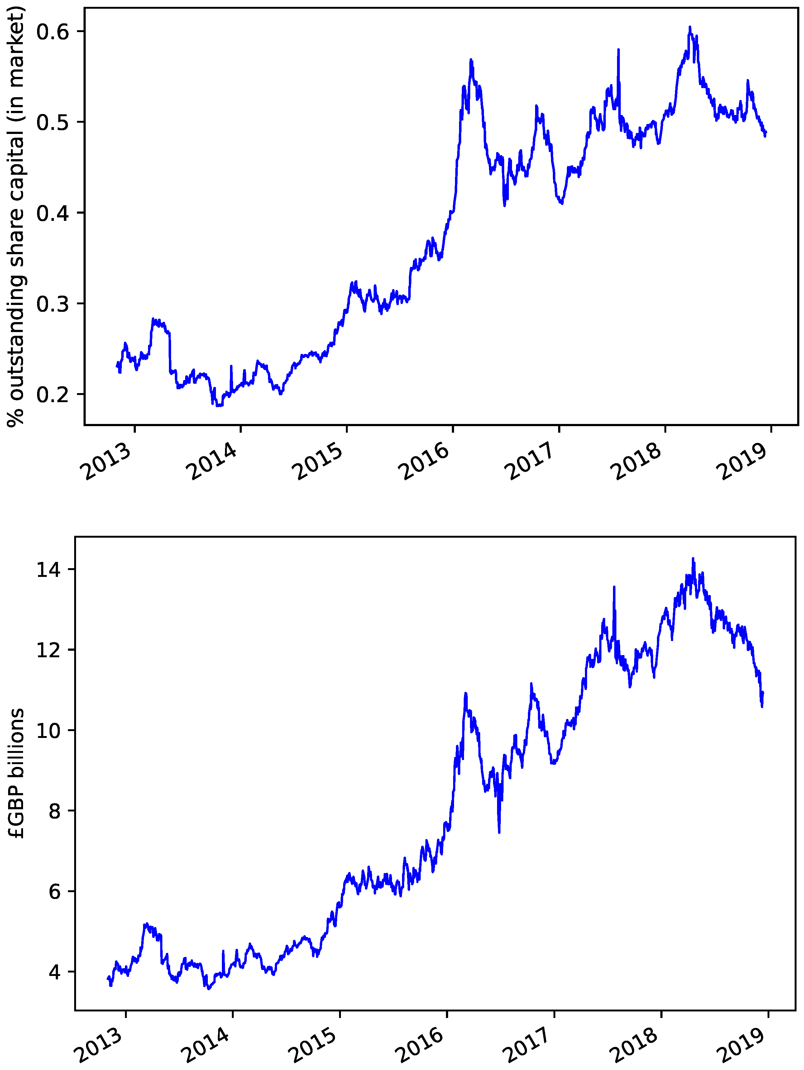
Figure 3.
Rolling window mean returns to long and short side of standard long-short portfolios. The 252-day rolling window mean return for both the long and short sides of the declared net short positions portfolios with value weights (“VW”), equal weights (“EW”), and net short position weights (“SW”). The mean return is scaled by 252 to make it an approximately annual figure. The date on the horizontal axis show the rolling window end. The first rolling window begins on 1 November 2013 and ends on 30 October 2014. The last rolling window ends on 13 December 2018.

Figure 4.
Rolling window t-statistic for standard long-short portfolios. HAC 252-day rolling window t-statistic on for the long-short declared net short positions portfolios with value weights (“VW”), equal weights (“EW”), and net short positions weights (“SW”). The date on the horizontal axis shows the rolling window end. The alphas are scaled by 252 to make them approximately annual figures. The first rolling window begins on 1 November 2013 and ends on 30 October 2014. The last rolling window ends on 13 December 2018.
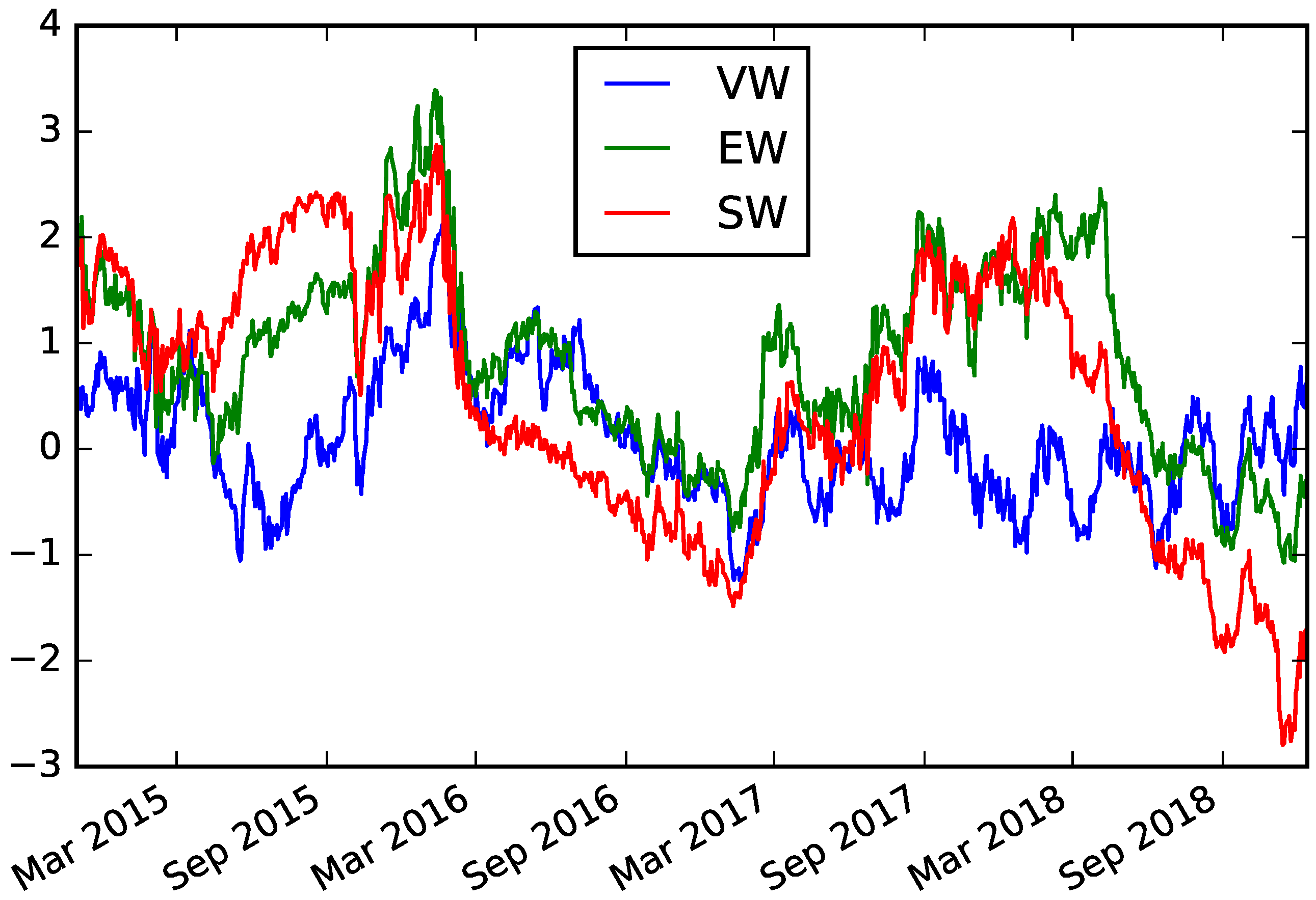
Figure 5.
Rolling window mean returns to equal-weighted fully invested and all-share portfolios. The 252-day rolling window mean return for the unconstrained (“UC”) and long-only (“LO”) fully invested portfolios, as well as the portfolio of all stocks (“AS”). The mean return is scaled by 252 to make it an approximately annual figure. The date on the horizontal axis shows the rolling window end. The first rolling window begins on 1 November 2013 and ends on 30 October 2014. The last rolling window ends on 13 December 2018.
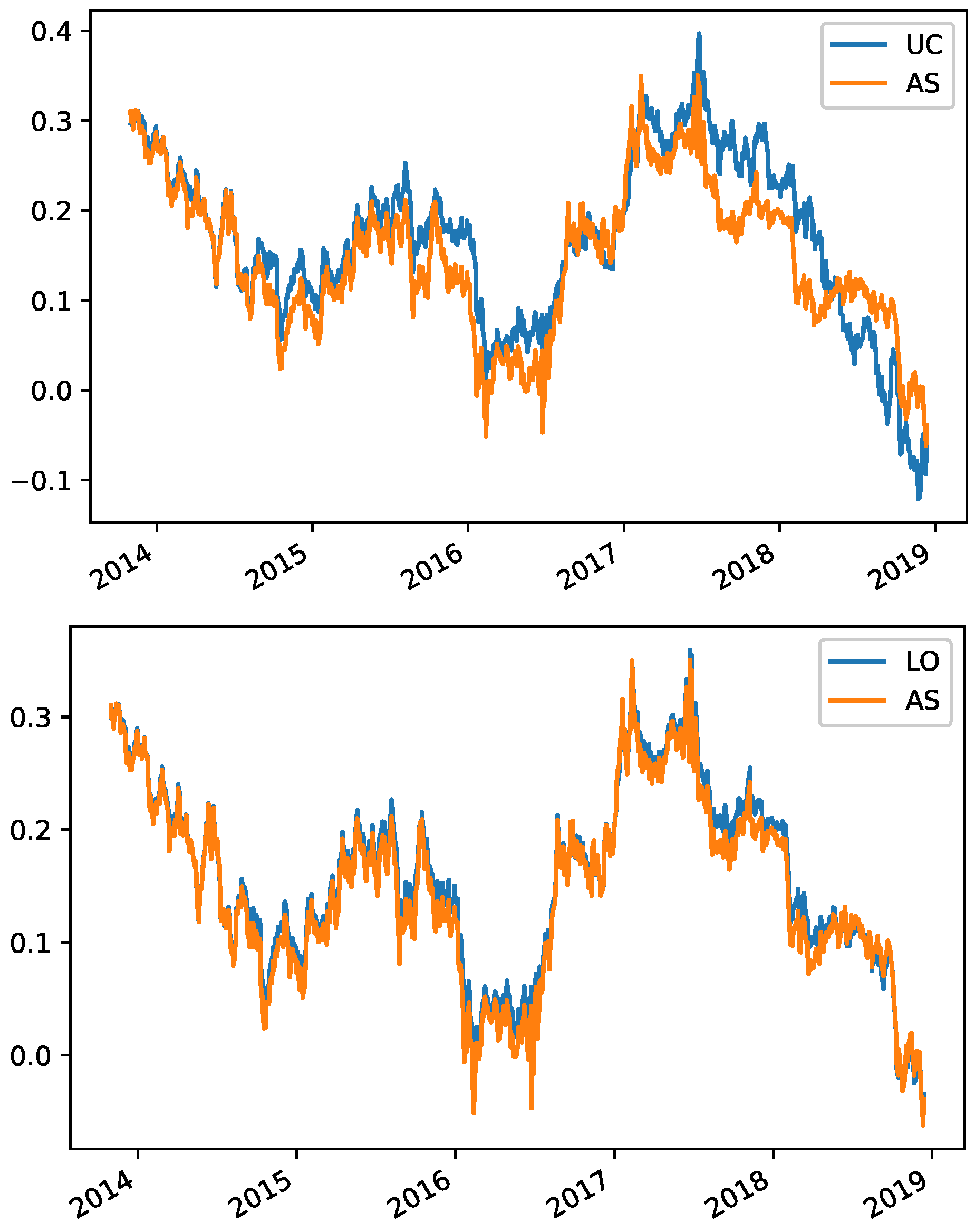
Table 1.
Summary statistics of public net short position disclosures.
| No. of Disclosures | Position Size | Duration | |||
|---|---|---|---|---|---|
| Per Day | Per Stock | % Outstanding Share Capital | GBP | Mean Days per Stock | |
| Mean | 18.9 | 29.7 | 0.94% | £30.5 mn | 49.2 |
| Median | 16.0 | 19.0 | 0.71% | £19.3 mn | 35.8 |
| Standard deviation | 13.1 | 30.4 | 0.68% | £44.5 mn | 49.5 |
| Maximum | 68.0 | 149 | 8.03% | £1443 mn | 529 |
| Minimum | 0.00 | 0.00 | 0.00% | £0.07 mn | 1.00 |
Summary statistics for the number of public net short position disclosures in FTSE350 listed stocks over the sample period (2 November 2012–13 December 2018). The first day of the regulations is excluded, as the declaration of existing positions opened before the regulations took effect is likely to distort the summary statistics. Disclosures include both declarations of positions that have just crossed the 0.5% reporting threshold and updates to positions which have already been declared as being above the threshold. Disclosures for a given stock are not aggregated across investors in the position size statistics. The standard deviation is computed using the unbiased estimator.
Table 2.
Standard long-short portfolio performance.
| Mean | p-Value | Sharpe | p-Value | p-Value | p-Value | ||||
|---|---|---|---|---|---|---|---|---|---|
| Value-weighted | |||||||||
| Long | 0.075 | 0.062 | 0.797 | 0.073 | 0.021 | 0.069 | 0.037 | 0.082 | 0.017 |
| Short | 0.053 | 0.401 | 0.377 | 0.055 | 0.275 | 0.065 | 0.193 | 0.070 | 0.184 |
| L-S | 0.022 | 0.491 | 0.415 | 0.018 | 0.519 | 0.004 | 0.873 | 0.012 | 0.658 |
| Equal-weighted | |||||||||
| Long | 0.119 | 0.007 | 1.170 | 0.118 | 0.001 | 0.114 | 0.002 | 0.127 | 0.001 |
| Short | 0.075 | 0.161 | 0.679 | 0.077 | 0.076 | 0.084 | 0.053 | 0.096 | 0.035 |
| L-S | 0.044 | 0.042 | 1.127 | 0.041 | 0.046 | 0.029 | 0.133 | 0.031 | 0.121 |
| Net short position-weighted | |||||||||
| Long | 0.119 | 0.007 | 1.170 | 0.118 | 0.001 | 0.114 | 0.002 | 0.127 | 0.001 |
| Short | 0.092 | 0.121 | 0.777 | 0.094 | 0.059 | 0.104 | 0.036 | 0.113 | 0.029 |
| L-S | 0.027 | 0.449 | 0.360 | 0.024 | 0.479 | 0.010 | 0.772 | 0.013 | 0.692 |
Performance evaluation measures for daily rebalanced declared net short position portfolios over the sample period 1 November 2013–13 December 2018. Means and alphas are scaled by 252 to make them approximately annual figures. Mean and alpha p-values are based on daily returns and are HAC. The Sharpe ratio is the annualised Sharpe ratio, allowing for serial correlation, computed as per Lo (2002).
Table 3.
Volatility scaled standard long-short portfolios with stop-loss rules.
| Monthly Rebalancing | |||||||||
| Mean | -Value | Sharpe | -Value | -Value | -Value | ||||
| Value-weighted | |||||||||
| Long | 0.051 | 0.140 | 0.647 | 0.048 | 0.078 | 0.039 | 0.178 | 0.050 | 0.093 |
| Short | 0.103 | 0.085 | 0.777 | 0.105 | 0.036 | 0.115 | 0.019 | 0.122 | 0.022 |
| L-S | −0.053 | 0.166 | −0.722 | −0.057 | 0.093 | −0.076 | 0.016 | −0.072 | 0.034 |
| Equal-weighted | |||||||||
| Long | 0.106 | 0.004 | 1.251 | 0.104 | 0.000 | 0.098 | 0.002 | 0.110 | 0.001 |
| Short | 0.028 | 0.607 | 0.209 | 0.029 | 0.518 | 0.040 | 0.359 | 0.049 | 0.298 |
| L-S | 0.078 | 0.030 | 1.009 | 0.075 | 0.026 | 0.058 | 0.062 | 0.061 | 0.062 |
| Net short position-weighted | |||||||||
| Long | 0.106 | 0.004 | 1.251 | 0.104 | 0.000 | 0.098 | 0.002 | 0.110 | 0.001 |
| Short | 0.030 | 0.641 | 0.199 | 0.032 | 0.564 | 0.046 | 0.391 | 0.052 | 0.359 |
| L-S | 0.076 | 0.154 | 0.674 | 0.072 | 0.142 | 0.053 | 0.260 | 0.058 | 0.215 |
| Annual Rebalancing | |||||||||
| Mean | -Value | Sharpe | -Value | -Value | -Value | ||||
| Value-weighted | |||||||||
| Long | 0.047 | 0.187 | 0.580 | 0.045 | 0.114 | 0.042 | 0.160 | 0.054 | 0.084 |
| Short | 0.113 | 0.040 | 0.977 | 0.114 | 0.013 | 0.118 | 0.010 | 0.127 | 0.009 |
| L-S | −0.066 | 0.029 | −1.245 | −0.068 | 0.014 | −0.076 | 0.005 | −0.072 | 0.009 |
| Equal-weighted | |||||||||
| Long | 0.104 | 0.006 | 1.225 | 0.102 | 0.001 | 0.098 | 0.002 | 0.111 | 0.001 |
| Short | 0.045 | 0.396 | 0.382 | 0.046 | 0.287 | 0.052 | 0.231 | 0.062 | 0.171 |
| L-S | 0.059 | 0.032 | 1.087 | 0.057 | 0.020 | 0.047 | 0.044 | 0.048 | 0.039 |
| Net short position-weighted | |||||||||
| Long | 0.104 | 0.006 | 1.225 | 0.102 | 0.001 | 0.098 | 0.002 | 0.111 | 0.001 |
| Short | 0.044 | 0.455 | 0.337 | 0.046 | 0.367 | 0.054 | 0.280 | 0.064 | 0.217 |
| L-S | 0.060 | 0.143 | 0.697 | 0.057 | 0.131 | 0.044 | 0.229 | 0.046 | 0.201 |
Performance evaluation measures for declared net short positions based portfolios over the sample period 1 November 2013–13 December 2018. Means and alphas are scaled by 252 days to make them approximately annual figures. Mean and alpha p-Values are based on daily returns and are HAC. The Sharpe ratio is the annualised Sharpe ratio, allowing for serial correlation, computed as per Lo (2002).
Table 4.
Performance of long-short portfolios based on multiple days’ disclosures.
| Mean | p-Value | Sharpe | p-Value | p-Value | p-Value | ||||
|---|---|---|---|---|---|---|---|---|---|
| Multiple signals approach | |||||||||
| Long | 0.107 | 0.008 | 1.133 | 0.105 | 0.001 | 0.101 | 0.002 | 0.113 | 0.001 |
| Short | 0.077 | 0.151 | 0.692 | 0.078 | 0.068 | 0.084 | 0.052 | 0.096 | 0.033 |
| L-S | 0.030 | 0.169 | 0.832 | 0.027 | 0.183 | 0.017 | 0.382 | 0.017 | 0.382 |
| Regression-based approach: Value weights | |||||||||
| Long | 0.099 | 0.025 | 0.957 | 0.099 | 0.007 | 0.098 | 0.009 | 0.110 | 0.004 |
| Short | 0.057 | 0.285 | 0.516 | 0.058 | 0.161 | 0.057 | 0.162 | 0.065 | 0.129 |
| L-S | 0.042 | 0.172 | 0.966 | 0.041 | 0.192 | 0.041 | 0.196 | 0.045 | 0.148 |
| Regression-based approach: Equal weights | |||||||||
| Long | 0.122 | 0.008 | 1.110 | 0.122 | 0.001 | 0.121 | 0.001 | 0.135 | 0.001 |
| Short | 0.067 | 0.179 | 0.660 | 0.067 | 0.084 | 0.065 | 0.103 | 0.078 | 0.058 |
| L-S | 0.056 | 0.017 | 1.118 | 0.055 | 0.015 | 0.056 | 0.010 | 0.057 | 0.011 |
| Regression-based approach: Expected return weights | |||||||||
| Long | 0.165 | 0.052 | 0.760 | 0.166 | 0.027 | 0.165 | 0.039 | 0.171 | 0.037 |
| Short | 0.066 | 0.342 | 0.451 | 0.065 | 0.264 | 0.067 | 0.260 | 0.076 | 0.187 |
| L-S | 0.099 | 0.262 | 0.500 | 0.101 | 0.255 | 0.098 | 0.276 | 0.095 | 0.297 |
Performance evaluation measures for daily rebalanced declared net short positions portfolios over the sample period 1 November 2013–13 December 2018. Means and alphas are scaled by 252 to make them approximately annual figures. Mean and alpha p-values are based on daily returns and are HAC. The Sharpe ratio is the annualised Sharpe ratio, allowing for serial correlation, computed as per Lo (2002).
Table 5.
Performance of volatility-scaled long-short portfolios based on multiple days’ declarations.
Table 5.
Performance of volatility-scaled long-short portfolios based on multiple days’ declarations.
| Mean | p-Value | Sharpe | p-Value | p-Value | p-Value | ||||
|---|---|---|---|---|---|---|---|---|---|
| Multiple signals approach | |||||||||
| Long | 0.113 | 0.002 | 1.376 | 0.111 | 0.000 | 0.106 | 0.000 | 0.117 | 0.000 |
| Short | 0.068 | 0.148 | 0.691 | 0.068 | 0.067 | 0.071 | 0.059 | 0.084 | 0.030 |
| L-S | 0.045 | 0.003 | 1.946 | 0.043 | 0.003 | 0.035 | 0.012 | 0.033 | 0.017 |
| Regression-based approach: Value weights | |||||||||
| Long | 0.081 | 0.037 | 0.899 | 0.080 | 0.011 | 0.077 | 0.019 | 0.089 | 0.008 |
| Short | 0.059 | 0.259 | 0.564 | 0.058 | 0.155 | 0.053 | 0.192 | 0.062 | 0.139 |
| L-S | 0.022 | 0.524 | 0.398 | 0.022 | 0.546 | 0.024 | 0.505 | 0.027 | 0.455 |
| Regression-based approach: Equal weights | |||||||||
| Long | 0.108 | 0.006 | 1.184 | 0.107 | 0.000 | 0.106 | 0.001 | 0.119 | 0.000 |
| Short | 0.062 | 0.157 | 0.687 | 0.062 | 0.070 | 0.057 | 0.109 | 0.069 | 0.052 |
| L-S | 0.046 | 0.005 | 1.617 | 0.045 | 0.004 | 0.049 | 0.002 | 0.050 | 0.001 |
| Regression-based approach: Expected return weights | |||||||||
| Long | 0.142 | 0.072 | 0.707 | 0.142 | 0.036 | 0.140 | 0.055 | 0.147 | 0.046 |
| Short | 0.047 | 0.470 | 0.317 | 0.045 | 0.395 | 0.046 | 0.405 | 0.057 | 0.269 |
| L-S | 0.095 | 0.202 | 0.608 | 0.097 | 0.195 | 0.094 | 0.223 | 0.090 | 0.248 |
Performance evaluation measures for daily rebalanced declared net short positions portfolios over the sample period 1 November 2013–13 December 2018. Means and alphas are scaled by 252 to make them approximately annual figures. Mean and alpha p-values are based on daily returns and are HAC. The Sharpe ratio is the annualised Sharpe ratio, allowing for serial correlation, computed as per Lo (2002).
Table 6.
Multiple signals portfolio performance with monthly rebalancing and stop-loss rules.
| No Volatility Scaling | |||||||||
| Mean | -Value | Sharpe | -Value | -Value | -Value | ||||
| Multiple signals approach | |||||||||
| Long | 0.112 | 0.011 | 1.200 | 0.115 | 0.001 | 0.112 | 0.001 | 0.122 | 0.001 |
| Short | 0.029 | 0.670 | 0.186 | 0.040 | 0.466 | 0.050 | 0.364 | 0.055 | 0.329 |
| L-S | 0.083 | 0.041 | 0.998 | 0.075 | 0.046 | 0.063 | 0.088 | 0.067 | 0.071 |
| With Volatility Scaling | |||||||||
| Mean | -Value | Sharpe | -Value | -Value | -Value | ||||
| Multiple signals approach | |||||||||
| Long | 0.117 | 0.004 | 1.364 | 0.120 | 0.000 | 0.116 | 0.001 | 0.126 | 0.000 |
| Short | 0.029 | 0.607 | 0.224 | 0.038 | 0.398 | 0.044 | 0.324 | 0.052 | 0.259 |
| L-S | 0.088 | 0.002 | 1.400 | 0.082 | 0.003 | 0.072 | 0.010 | 0.074 | 0.009 |
Performance evaluation measures for declared net short positions portfolios over the sample period 1 November 2013–13 December 2018. Means and alphas are scaled by 252 days to make them approximately annual figures. Mean and alpha p-values are based on daily returns and are HAC. The Sharpe ratio is the annualised Sharpe ratio, allowing for serial correlation, computed as per Lo (2002).
Table 7.
Fully invested portfolios using the most recent day’s declarations —daily rebalancing.
| Fully Invested Portfolios | |||||||||||
| Mean | -Value | Sharpe | -Value | -Value | -Value | Turn | MDD | ||||
| Equal-weighted | |||||||||||
| UC | 0.129 | 0.006 | 1.085 | 0.126 | 0.001 | 0.114 | 0.006 | 0.126 | 0.003 | 0.070 | 0.160 |
| LO | 0.117 | 0.009 | 1.151 | 0.116 | 0.001 | 0.112 | 0.002 | 0.125 | 0.001 | 0.009 | 0.127 |
| AS | 0.108 | 0.019 | 1.059 | - | - | - | - | - | - | 0.000 | 0.139 |
| Value-weighted | |||||||||||
| UC | 0.054 | 0.129 | 0.665 | 0.051 | 0.072 | 0.042 | 0.159 | 0.055 | 0.072 | 0.032 | 0.139 |
| LO | 0.072 | 0.075 | 0.760 | 0.070 | 0.027 | 0.065 | 0.048 | 0.079 | 0.022 | 0.013 | 0.155 |
| AS | 0.079 | 0.068 | 0.783 | - | - | - | - | - | - | 0.009 | 0.167 |
| Differences between Portfolios | |||||||||||
| Mean | -Value | Sharpe | -Value | -Value | -Value | ||||||
| Equal-weighted | |||||||||||
| UC-AS | 0.022 | 0.358 | 0.525 | 0.019 | 0.461 | 0.009 | 0.713 | 0.008 | 0.749 | ||
| LO-AS | 0.010 | 0.038 | 1.266 | 0.009 | 0.062 | 0.007 | 0.160 | 0.007 | 0.157 | ||
| UC-LO | 0.012 | 0.536 | 0.349 | 0.010 | 0.644 | 0.003 | 0.903 | 0.001 | 0.953 | ||
| Value-weighted | |||||||||||
| UC-AS | −0.025 | 0.159 | −0.749 | −0.027 | 0.104 | −0.034 | 0.049 | −0.034 | 0.045 | ||
| LO-AS | −0.008 | 0.191 | −0.744 | −0.008 | 0.126 | −0.011 | 0.057 | −0.011 | 0.052 | ||
| UC-LO | −0.018 | 0.147 | −0.744 | −0.019 | 0.097 | −0.024 | 0.047 | −0.024 | 0.043 | ||
| Expected Shortfalls (Daily Returns) | |||||||||||
| Equal-weighted | |||||||||||
| UC | 0.029 | 0.016 | 0.012 | ||||||||
| LO | 0.028 | 0.016 | 0.012 | ||||||||
| AS | 0.030 | 0.017 | 0.013 | ||||||||
| Value-weighted | |||||||||||
| UC | 0.031 | 0.018 | 0.014 | ||||||||
| LO | 0.030 | 0.018 | 0.014 | ||||||||
| AS | 0.032 | 0.019 | 0.014 | ||||||||
Performance evaluation measures for fully invested portfolios over the sample period 1 November 2013–13 December 2018. Means and alphas are scaled by 252 days to make them approximately annual figures. Mean and alpha p-values are based on daily returns and are HAC. The Sharpe ratio is the annualised Sharpe ratio, allowing for serial correlation, computed as per Lo (2002). “Turn” denotes daily turnover and “MDD” maximum drawdown. The top panel shows the mean gross and risk-adjusted returns to the unconstrained (UC), long-only (LO), and all-stock (AS) portfolios in isolation. Alphas are not reported for the all-share portfolios since the risk models all contain a market factor. In the middle panel, row “X-Y” shows the difference in returns between X and Y. The Sharpe ratio is the Sharpe ratio of a portfolio which is GBP 1 long in X and GBP 1 short in Y. The bottom panel shows the expected shortfall at the 99% (), 95% (), and 90% () level.
Table 8.
Fully invested portfolios using multiple days’ declarations—daily rebalancing.
| Fully Invested Portfolios | |||||||||||
| Mean | -Val | Sharpe | -Val | -Val | -Val | Turn | MDD | ||||
| Equal-weighted | |||||||||||
| UC | 0.123 | 0.004 | 1.276 | 0.118 | 0.003 | 0.104 | 0.010 | 0.105 | 0.014 | 0.102 | 0.256 |
| LO | 0.107 | 0.008 | 1.135 | 0.105 | 0.001 | 0.101 | 0.002 | 0.112 | 0.001 | 0.005 | 0.119 |
| AS | 0.108 | 0.019 | 1.059 | - | - | - | - | - | - | 0.000 | 0.139 |
| Value-weighted | |||||||||||
| UC | 0.052 | 0.125 | 0.696 | 0.049 | 0.083 | 0.039 | 0.191 | 0.051 | 0.087 | 0.031 | 0.136 |
| LO | 0.073 | 0.069 | 0.771 | 0.071 | 0.026 | 0.066 | 0.046 | 0.079 | 0.022 | 0.011 | 0.155 |
| AS | 0.079 | 0.068 | 0.783 | - | - | - | - | - | - | 0.009 | 0.167 |
| Differences between Portfolios | |||||||||||
| Mean | -Val | Sharpe | -Val | -Val | -Val | ||||||
| Equal-weighted | |||||||||||
| UC-AS | 0.016 | 0.688 | 1.035 | 0.011 | 0.788 | −0.001 | 0.987 | −0.013 | 0.732 | ||
| LO-AS | −0.001 | 0.895 | −0.085 | −0.002 | 0.772 | −0.004 | 0.555 | −0.005 | 0.449 | ||
| UC-LO | 0.017 | 0.618 | 1.874 | 0.013 | 0.710 | 0.004 | 0.915 | −0.007 | 0.815 | ||
| Value-weighted | |||||||||||
| UC-AS | −0.027 | 0.185 | −0.689 | −0.030 | 0.115 | −0.037 | 0.064 | −0.038 | 0.053 | ||
| LO-AS | −0.006 | 0.296 | −0.618 | −0.007 | 0.206 | −0.009 | 0.110 | −0.010 | 0.084 | ||
| UC-LO | −0.021 | 0.159 | −0.690 | −0.022 | 0.097 | −0.028 | 0.058 | −0.028 | 0.050 | ||
| Expected Shortfalls (Daily Returns) | |||||||||||
| Equal-weighted | |||||||||||
| UC | 0.026 | 0.014 | 0.011 | ||||||||
| LO | 0.038 | 0.021 | 0.015 | ||||||||
| AS | 0.030 | 0.017 | 0.013 | ||||||||
| Value-weighted | |||||||||||
| UC | 0.031 | 0.018 | 0.014 | ||||||||
| LO | 0.030 | 0.018 | 0.015 | ||||||||
| AS | 0.032 | 0.019 | 0.014 | ||||||||
Performance evaluation measures for fully invested portfolios over the sample period 1 November 2013–13 December 2018. Means and alphas are scaled by 252 days to make them approximately annual figures. Mean and alpha p-values are based on daily returns and are HAC. The Sharpe ratio is the annualised Sharpe ratio, allowing for serial correlation, computed as per Lo (2002). “Turn” denotes daily turnover and “MDD” maximum drawdown. The top panel shows the mean gross and risk-adjusted returns to the unconstrained (UC), long-only (LO), and all-stock (AS) portfolios in isolation. Alphas are not reported for the all-share portfolios since the risk models all contain a market factor. In the middle panel, row “X-Y” shows the difference in returns between X and Y. The Sharpe ratio is the Sharpe ratio of a portfolio which is GBP 1 long in X and GBP 1 short in Y. The bottom panel shows the expected shortfall at the 99% (), 95% (), and 90% () level.
Table 9.
Fully invested portfolios using multiple days’ declarations—daily rebalancing and volatility scaling.
Table 9.
Fully invested portfolios using multiple days’ declarations—daily rebalancing and volatility scaling.
| Fully Invested Portfolios | |||||||||||
| Mean | -Val | Sharpe | -Val | -Val | -Val | Turn | MDD | ||||
| Equal-weighted | |||||||||||
| UC | 0.129 | 0.000 | 1.613 | 0.125 | 0.000 | 0.117 | 0.000 | 0.124 | 0.000 | 0.066 | 0.090 |
| LO | 0.109 | 0.003 | 1.321 | 0.107 | 0.000 | 0.103 | 0.001 | 0.113 | 0.000 | 0.019 | 0.104 |
| AS | 0.097 | 0.013 | 1.111 | - | - | - | - | - | - | 0.015 | 0.118 |
| Value-weighted | |||||||||||
| UC | 0.065 | 0.061 | 0.819 | 0.062 | 0.030 | 0.053 | 0.070 | 0.063 | 0.035 | 0.034 | 0.126 |
| LO | 0.072 | 0.052 | 0.846 | 0.069 | 0.019 | 0.064 | 0.038 | 0.075 | 0.017 | 0.016 | 0.142 |
| AS | 0.076 | 0.084 | 0.738 | - | - | - | - | - | - | 0.009 | 0.169 |
| Differences between Portfolios | |||||||||||
| Mean | -Val | Sharpe | -Val | -Val | -Val | ||||||
| Equal-weighted | |||||||||||
| UC-AS | 0.032 | 0.029 | 1.350 | 0.030 | 0.050 | 0.024 | 0.118 | 0.019 | 0.190 | ||
| LO-AS | 0.012 | 0.005 | 1.566 | 0.012 | 0.005 | 0.010 | 0.015 | 0.009 | 0.032 | ||
| UC-LO | 0.020 | 0.065 | 1.196 | 0.018 | 0.111 | 0.014 | 0.229 | 0.010 | 0.338 | ||
| Value-weighted | |||||||||||
| UC-AS | −0.010 | 0.528 | −0.365 | −0.013 | 0.384 | −0.019 | 0.212 | −0.022 | 0.138 | ||
| LO-AS | −0.004 | 0.686 | −0.202 | −0.005 | 0.523 | −0.008 | 0.361 | −0.010 | 0.261 | ||
| UC-LO | −0.006 | 0.402 | −0.600 | −0.007 | 0.322 | −0.011 | 0.137 | −0.012 | 0.088 | ||
Performance evaluation measures for volatility-scaled fully invested portfolios over the sample period 1 November 2013–13 December 2018. Means and alphas are scaled by 252 days to make them approximately annual figures. Mean and alpha p-values are based on daily returns and are HAC. The Sharpe ratio is the annualised Sharpe ratio, allowing for serial correlation, computed as per Lo (2002). “Turn” denotes daily turnover and “MDD” maximum drawdown. The top panel shows the mean gross and risk-adjusted returns to the unconstrained (UC), long-only (LO), and all-stock (AS) portfolios in isolation. Alphas are not reported for the all-share portfolios since the risk models all contain a market factor. In the middle panel, row “X-Y” shows the difference in returns between X and Y. The Sharpe ratio is the Sharpe ratio of a portfolio which is GBP 1 long in X and GBP 1 short in Y.
Table 10.
Value-weighted long-short portfolios using closing prices.
| Mean | p-Val | Sharpe | p-Val | p-Val | p-Val | ||||
|---|---|---|---|---|---|---|---|---|---|
| Value-weighted portfolio based on most recent day’s declaration | |||||||||
| Long | 0.082 | 0.040 | 0.882 | 0.068 | 0.049 | 0.056 | 0.131 | 0.082 | 0.027 |
| Short | 0.012 | 0.855 | 0.059 | 0.014 | 0.743 | 0.036 | 0.417 | 0.047 | 0.271 |
| L-S | 0.070 | 0.048 | 1.110 | 0.054 | 0.152 | 0.020 | 0.579 | 0.035 | 0.361 |
| Value-weighted regression-based portfolio | |||||||||
| Long | 0.124 | 0.008 | 1.176 | 0.112 | 0.001 | 0.110 | 0.003 | 0.133 | 0.000 |
| Short | 0.041 | 0.454 | 0.359 | 0.037 | 0.364 | 0.041 | 0.328 | 0.055 | 0.187 |
| L-S | 0.083 | 0.009 | 1.729 | 0.076 | 0.004 | 0.069 | 0.005 | 0.078 | 0.002 |
Daily rebalanced portfolios over the sample period 1 November 2013–13 December 2018. Performance evaluation measures for declared net short positions portfolios. Means and alphas are scaled by 252 days to make them approximately annual figures. Mean and alpha p-values are based on daily returns and are HAC. The Sharpe ratio is the annualised Sharpe ratio, allowing for serial correlation, computed as per Lo (2002).
Table 11.
Value-weighted long-short portfolios using day-t closing prices and day-t declarations.
| Mean | p-Val | Sharpe | p-Val | p-Val | p-Val | ||||
|---|---|---|---|---|---|---|---|---|---|
| Non-volatility-scaled | |||||||||
| Long | 0.082 | 0.040 | 0.880 | 0.068 | 0.049 | 0.056 | 0.132 | 0.082 | 0.027 |
| Short | −0.001 | 0.986 | −0.034 | 0.003 | 0.955 | 0.034 | 0.535 | 0.041 | 0.449 |
| L-S | 0.084 | 0.119 | 0.896 | 0.065 | 0.226 | 0.022 | 0.656 | 0.042 | 0.432 |
| Volatility-scaled | |||||||||
| Long | 0.081 | 0.038 | 0.905 | 0.065 | 0.069 | 0.050 | 0.183 | 0.072 | 0.053 |
| Short | −0.006 | 0.932 | −0.071 | −0.007 | 0.888 | 0.013 | 0.796 | 0.022 | 0.651 |
| L-S | 0.087 | 0.017 | 1.291 | 0.072 | 0.102 | 0.037 | 0.375 | 0.050 | 0.250 |
Daily rebalanced portfolios over the sample period 1 November 2013–13 December 2018. Performance evaluation measures for declared net short position portfolios. Means and alphas are scaled by 252 days to make them approximately annual figures. Mean and alpha p-values are based on daily returns and are HAC. The Sharpe ratio is the annualised Sharpe ratio, allowing for serial correlation, computed as per Lo (2002).
Disclaimer/Publisher’s Note: The statements, opinions and data contained in all publications are solely those of the individual author(s) and contributor(s) and not of MDPI and/or the editor(s). MDPI and/or the editor(s) disclaim responsibility for any injury to people or property resulting from any ideas, methods, instructions or products referred to in the content. |
© 2024 by the author. Licensee MDPI, Basel, Switzerland. This article is an open access article distributed under the terms and conditions of the Creative Commons Attribution (CC BY) license (https://creativecommons.org/licenses/by/4.0/).
Share and Cite
MDPI and ACS Style
Ashby, M. Are Regulatory Short Sale Data a Profitable Predictor of UK Stock Returns? J. Risk Financial Manag. 2024, 17, 320. https://doi.org/10.3390/jrfm17080320
AMA Style
Ashby M. Are Regulatory Short Sale Data a Profitable Predictor of UK Stock Returns? Journal of Risk and Financial Management. 2024; 17(8):320. https://doi.org/10.3390/jrfm17080320
Chicago/Turabian StyleAshby, Michael. 2024. "Are Regulatory Short Sale Data a Profitable Predictor of UK Stock Returns?" Journal of Risk and Financial Management 17, no. 8: 320. https://doi.org/10.3390/jrfm17080320