Abstract
The paper analyses optimal spending of an endowment fund. The purpose is to find a spending rule which is optimal for the owners and which secures that the fund will last “forever”. This we do by finding closed form solutions of the optimal consumption to wealth ratio. We solve this problem using the life cycle model, where the agent can have preferences represented by expected utility or recursive utility. We apply our results to a sovereign wealth fund, and demonstrate that the optimal spending rate is significantly lower than the fund’s expected real rate of return, a rule which is in common use. Employing the latter as the spending rate, implies that the fund’s value deteriorates both in probability and in expectation, as time goes. For both kinds of long term convergence we find closed form threshold values. Spending below these values secures a sustainable fund.
Keywords:
life cycle model; optimal spending rate; endowment funds; expected utility; recursive utility; risk aversion; EIS; consumption to wealth ratio; almost sure convergence; 1st mean convergence; first order stochastic dominance JEL Classification:
G10; G12; D9; D51; D53; D90; E21
1. Introduction
We consider optimal investment strategies and optimal spending from an endowment fund consistent with the life cycle model. It turns out that the optimal spending rate is, for reasonable values of the preference parameters, strictly smaller than the expected rate of return, and the difference is significant.
According to Eeckhoudt et al. (2005) is preference for diversification intrinsically equivalent to risk aversion. In contrast, extracting the expected real rate of return on a fund is associated to risk neutrality.
A nation is sometimes considered to be risk neutral when compared to the individuals of society. This follows from the theory of syndicates (see, for example, Borch 1960, 1962). When a nation has decided to invest broadly in the world’s financial markets, this means that it considers itself to be risk averse in relation to these markets, which represent values much larger than the nation’s wealth.
We take the security market as given, assumed to be in a dynamic equilibrium, and introduce a price taking agent in this market. In this setting we reconsider the problem of optimal consumption and portfolio selection to obtain closed form solutions. In the context of an endowment fund, the results from analyzing this more general problem we immediately use to determine an optimal spending rate defined as the consumption to wealth ratio. To represent preferences we use both expected utility (EU) as well as recursive utility (RU), where for RU intertemporal substitution of consumption is separated from risk aversion. This separation property turns out to be both clarifying and useful in our analysis.
The microfoundation of adopting utility functions in contexts like this has been discussed in the literature, and seems well founded (see for example, Blanchard 1985). In some interpretations this requires a constant population.
When the investment opportunity set is deterministic, meaning that crucial parameters of the analysis are non-stochastic, there exist explicit and closed form solutions for optimal spending in the continuous-time model (Merton 1969, 1971). This was utilized in Aase and Bjerksund (2021), who also extended the analysis to a stochastic investment opportunity set, that is, key parameters in the financial market are allowed to be random.
In the discrete-time model closed form solutions are hard to come across. The early papers by Mossin (1968), and Samuelson (1969) realized that dynamic programming can be used, but this did not lead to closed form solutions. We have used directional derivatives to first find the optimal consumption subject to a budget constraint. With a closed form solution to this problem, we next solved the optimal portfolio selection problem by maximizing the remaining utility at each time t.
When finding closed form solutions to the optimal consumption to wealth ratio, we relied on first having formulated an appropriate model of the financial market. This model is inspired from the no-arbitrage theory following the seminal paper by Black and Scholes (1973). This breakthrough was in a continuous-time setting, but soon afterwards several papers, and books, followed using a discrete time framework, see for example Cox and Rubinstein (1985) and Skiadas (2009).
If the extraction rate is the one of expected return, this normally means that the agent is risk neutral at the level of spending, and must then, to be consistent, be risk neutral at the level of optimal portfolio selection as well. But the consequence of such an investment strategy is rarely advocated by anyone responsible for an endowment fund, whatever its purpose.
We demonstrate that a particular spending policy, the expected real rate of the fund, is not consistent with a reasonable long term development of the fund, and will with probability one eventually deteriorate any fund that is managed by diversification. In addition, the expected value of the fund will systematically decrease as time goes. Under stylised conditions we find closed form threshold values for both kinds of long term developments.
Many endowment funds share the perspective that they should last “forever”. Consequently, there is a trade-off between current spending and future spending opportunities. Tobin (1974) develop sustainable spending rules in a deterministic world. It can be argued that it is sustainable to spend the real interest rate (or something slightly smaller) within this setting.
Uncertainty complicates this picture. It has been argued that it is sustainable for an endowment fund to spend the expected fund return, see e.g., Campbell (2012), who considered university endowments. Moreover, this idea motivates the current 3% fiscal rule that applies to the 1 trillion USD Norwegian sovereign wealth fund.
Our article is concerned with optimal extraction of endowment funds in general, and has in particular been motivated by the Norwegian Government Pension Fund Global, earlier called the Norwegian Oil Fund or just the Norwegian sovereign wealth fund, which we consider as an example of the general theory. This case is considered in Section 9 of the paper.
In this connection it is worth noticing that the Norwegian Parliament has decided that the fund should last “forever”. Also, the extraction rule which is adopted is that of spending the real rate of return on the fund.
In this paper we show that that employing this rule, the fund will deteriorate to zero with probability 1 in the long run.
This looks like a version of “doublethink”, a concept in George Orwell’s novel 1984, namely the ability to have two conflicting beliefs in one’s mind at once, and accept both.
Related Literature
Dybvig and Qin (2019) consider a fund with normal iid log-returns. The authors find that for the fund to last “forever”, spending must not exceed expected fund return subtracted by half the variance.
The two key decisions of an endowment fund that invests in the financial market is how much risk to take and how much to spend. From a theoretical point of view, the two decisions are closely related and must be determined jointly. To examine the questions one must address the issue of the objective function by which optimality is to be measured. Merton (1971) presents optimal portfolio and consumption rules for an investor who maximizes expected, additive and separable utility with constant relative risk aversion in a continuous-time world, where risky asset returns are iid. Recursive utility is a more generalized framework where the investor’s risk aversion and consumption substitution are disentangled, see, e.g., Epstein and Zin (1991).
Campbell and Sigalov (2020) adopt the Merton model as well as Epstein-Zin preferences, and assume that there is a constraint on the spending rule. The authors examine two alternative constraints: (i) spending the expected return; and (ii) the maximum sustainable spending follows the assumption of Dybvig and Qin (2019). The authors find that the constraint induces increased risk taking (referred to as “reaching out for yield”).
Campbell and Martin (2022) introduce a sustainability constraint that the representative agent may choose to impose on herself. They view sustainability as a requirement that welfare should not be expected to decline over time. The constraint imposes an upper bound on the consumption to wealth ratio, which is shown to lie between the riskless rate and the expected return on optimally invested wealth. The constraint requires that the time t-conditional expected utility should not be allowed to decline, in expectation, over time. Also we consider utility as a stochastic process, but we do not constrain it. Rather we study the long term developments of the fund value itself under various assumptions on spending.
In Merton (1990, ch 21), optimal investment strategies for university endowment funds are analyzed, where the objective is maximization of expected utility, related to several activities consistent with the purposes of the university. We limit the scope to how much to optimally spend in the numeraire unit of account, which is a purely financial question. How much to spend on each of several activities we consider as a political issue.
One purpose of this paper is to compare the optimal spending with the conventional wisdom of spending the expected return, or any other ad hoc rule, under various assumptions. For this reason, we adopt and develop the life cycle model, where we consider the recursive utility framework in addition to the standard expected utility, in the setting of discrete time. Under specific conditions we find two threshold values that spending should not exceed, in order for the fund value to be maintained in the long run in a probabilistic sense. These values are independent of the agent’s preferences. We then demonstrate that, when the agent is reasonably patient, the optimal consumption to wealth ratio passes the two long run tests. If the spending rate is set equal to the expected rate of return on the endowment fund, both tests fail and the time development of the fund is negative.
The paper is organized as follows: The basic discrete-time model is formulated in Section 2. In Section 3 we solve the optimal consumption and portfolio choice problem with expected utility, and in Section 4 we find the corresponding optimal consumption to wealth ratio. In Section 5 we consider the asymptotic behaviour of a sovereign wealth fund. Numerical illustrations for expected utility follow in Section 6. In Section 7 we solve the optimal consumption and portfolio choice problem for recursive utility, and in Section 8 we present numerical illustrations for recursive utility. In Section 9 we consider the Norwegian SWF Government Fund Global, and in Section 10 we present more realistic, and also more general, asymptotics. Section 11 concludes. The paper contains 5 appendices where some of the the technical material and proofs can be found.
2. The Basic Financial Model
In this paper we are concerned with the optimal spending from a sovereign wealth fund, which we interpret as finding the optimal consumption to wealth ratio. Towards this end, we first consider the optimal consumption and portfolio selection problem using the life cycle model.
We have an agent represented by the pair , where is the agent’s utility function over consumption processes c, and e is the agent’s endowment process. The problem consists in maximizing utility subject to the agent’s budget constraint
where are the optimal fractions of wealth in the various risky investment possibilities facing the agent, and w is the current value of the agent’s wealth. The quantity is the state price at time t, i.e., the Arrow-Debreu state prices in units of probability. The horizon is .
The consumer takes as given a dynamic financial market in equilibrium, consisting of N risky securities and one riskless asset, the latter with rate of return , a stochastic process. The agent’s actions do not affect market prices of the risky assets, nor the risk-free rate of return .
The equilibrium referred to is a security-spot market equilibrium where the agents optimize utility, and the security prices, probabilities and the consumption price are determined such that markets clear. Prices and probabilities are endogenous, preferences are exogenous. In such an equilibrium there are no arbitrage possibilities, a property we will make repeated use of in the following. For details see, for example, Duffie (2001).
Preliminaries
We first assume that U represented separable and additive expected utility.
We address the same basic problem as the continuous-time paper by Aase and Bjerksund (2021), but we deviate on several accounts. First, the agent’s preferences are represented as
Here is the agent’s felicity index, which we assume to be of the CRRA-type, meaning that the real function , where is the agent’s relative risk aversion and is the agent’s patience factor (the utility discount factor). The parameters and are constants satisfying and . In continuous-time models , where is the impatience rate, . In our model we define the impatience rate more naturally from the relationship .
However, in a dynamic setting the interpretation of the parameter can also be the following, namely the agent’s resistance to intertemporal substitution of consumption. This property has little to do with risk aversion, which makes sense also in a one-period model.1
Recursive utility is treated in Section 7. The advantage with this form of preferences is that the two interpretations given to will now be separated, so that a new parameter will have the consumption substitution interpretation, while the parameter will represent relative risk aversion.
The introduction of preference parameters allows us to precent explicit results, and it is generally believed that this approach is fairly robust for the utility functions used in this paper (modulo the above objection to EU).
From the general theory in Appendix A we have that optimal consumption and the optimal wealth at time are connected as follows
Here is the conditional expectation of any random variable X given the information by time t, where , is the information filtration, , and , the Arrow-Debreu state price in units of probability, will be characterized in Appendix A.
The following model of the financial market is a discrete-time version of the theory that emerged after the no-arbitrage theory of contingent claims analysis had been established, motivated by the seminal paper of Black and Scholes (1973). Its aim is to characterize complete financial markets with no arbitrage possibilities. In such a market our agent operates as a price taker. There is by now an extensive literature on this topic, primarily in a continuous-time setting. The presentation in Appendix A is adapted from Skiadas (2009), see also Aase (2017). With the aid of this, we next focus on the predictions of the standard expected utility model.
3. Solution of the Consumption and Investment Problem with Expected Utility
In this section we treat the optimal consumption and optimal investment problem in our model. We start with the consumption problem.
3.1. Optimal Consumption Choice
We want to solve problem (1), where is given by (2). The Lagrangian for this problem is
where is the Lagrangian multiplier. We use Kuhn-Tucker with the Lagrange function given above, which reduces the problem to an unconstrained maximization problem. We find the first order condition using directional derivatives in function space (Gateaux derivatives), and finally we determine the Lagrange multiplier that yields equality in the budget constraint, which must hold since is strictly increasing in x. The Saddle Point Theorem provides the final solution. Alternatively, we could have employed dynamic programming based on the wealth Equation (A6) given in Appendix A.
Denoting the directional derivative of in the direction c by , the first order condition for this unconstrained problem is
where is the Lagrange multiplier for the wealth constraint. Here the optimal consumption path is assumed to exist, and we can ignore the positivity constraint on c because of the behaviour of when x approaches zero. We then obtain that
which implies that
where prime means derivative with respect to the first variable. Using the functional form of u, we find
From (8) we see that the optimal consumption is exposed to market movements only: When the state price is down, times are ‘good’ and consumption is high, and vice versa when the state price is up, consumption goes down. However, consumer spending tends to stay fairly stable, presumably because consumers use wealth to dampen the market variations. This is better explained by use of non-expected utility, which we return to below.
The property expressed in (8) is seen to hold for all consumers with CRRA utility, whatever the value of the -parameter so long as it is strictly positive. Equation (8) expresses a version of the mutuality principle (e.g., Borch 1960, 1962 and Wilson 1968): When the market is down, it is down for everyone and everyone consumes less (but to a varying degree), and vice versa everyone consumes more when the market is up.
When there is no market uncertainty, i.e., when for all , the model is known as the Ramsey model, see Ramsey (1928), Koopmans (1960).
3.2. The Associated Optimal Portfolio Selection Problem
Next we turn to the investment policy that goes along with the optimal consumption strategy of the the model presented in Appendix A.
Mossin (1968) was one of the first to study the problem of optimal investments. He leaves out intermediate consumption, i.e., consumption only takes place in the final period, and considers two assets, one risky and one risk-free. With CRRA-utility, he demonstrated that the optimal fraction of wealth held in the risky asset is constant across time provided returns are iid. He uses dynamic programming, as does Samuelson (1969) for the same problem, except that the latter author allows consumption in every period. Neither of these authors arrive at explicit formulas for general CRRA utility, but Samuelson is concerned with the special case .
Let us return to the optimal consumption solving problem (1) and characterized in Section 3.1. In the present model it is known that the the optimal consumption is proportional to wealth for expected utility, so that where is optimal wealth. Provided we limit ourselves to a deterministic investment opportunity set, where the parameters in the set are deterministic, the factor is deterministic, which we now assume. Here is the vector of conditional expected excess rates of return on the N risky securities in the market, while is the market-price-of-risk process, defined in Appendix A.
Let be the (simple) returns on the N risky assets, and is the (simple) return on the risk-free asset. Since solves the constrained optimization problem of Section 3.1, the optimal portfolio weights at time t for the next period solve the following problem , or
where
From our assumptions, this problem reduces to solving the following
Implied by our notation is that is -measurable. The first order condition is
Provided the product is small enough, by a Taylor series approximation it follows that
which, when return distributions are independent and stationary over time, implies that the ratios are constant over time. The inverse matrix in this expression is based on excess returns instead of the expected square deviations and is therefore not identical to the covariance matrix found in the continuous time analysis. This means that will be lower for the discrete time model but the difference is small. However, as we see below, the corresponding adjustments in the matrix in (11) implies that the consumption to wealth ratio is approximately the same in both models, as the matter must be. Under the same type of assumptions, there should be no real economic difference between the predictions of these two approaches.
In the continuous-time model , where and the product can be shown to satisfy . Similarly we can show that . We can also link the market-price-of-risk inner product to the optimal portfolio ratios for the continuous-time model and given in (11) via . This is demonstrated as follows.
In order to find M from we can use the concept of “bias” in statistical estimation theory, which gives the connection
Having solved the optimal consumption and portfolio selection problem in the life cycle model for expected additive and separable utility, we can now use this to find the optimal spending rate as the consumption to wealth ratio for an endowment fund. This we do in the next section.
4. The Optimal Consumption to Wealth Ratio
We now address the optimal spending problem of a sovereign wealth fund. First we prove the following result:
Theorem 1.
The connection between the optimal wealth and the optimal consumption at any time t is given by the following relationship:
The proof can be found in Appendix B.
In order to progress further, we need some simplifying assumptions. From now on we adopt the assumption of Section 3.2 of a stationary and deterministic investment opportunity set for all t. In order to compare our results to the associated continuous-time version, we also assume that are independent for , and independent and identically distributed across time t for each i.
Let , for all , . In order for the model to be complete, these variables are discretely distributed with state probabilities , summing to 1, and satisfying
If we assume we can neglect moments of order three and higher, we can simplify using Taylor series approximations. This gives the following result:
Theorem 2.
(a) Consider the finite horizon case . Under the above assumptions the optimal consumption to wealth ratio can be written as follows:
(b) Consider the infinite horizon case where . The optimal consumption to wealth ratio is given by
provided .
The proof can be found in Appendix B.
Remark 1.
By using Taylor approximations of the exponential function and the logarithmic function, we can write the above formula for as follows
The right-hand side is the exact formula for the optimal spending found in Equation (16) in Aase and Bjerksund (2021) for the continuous-time model, where the impatience rate . This expression can be seen to be a convex combination of the impatience rate δ and the certainty equivalent rate of return on the fund. The derivation can be found in Appendix A.
Remark 2.
For reasonable values of the preference parameters one can verify that the expected return on the fund is larger than the consumption to wealth ratio. We formalize this as follows:
Proposition 1.
The expected real rate of return on the fund is larger than the consumption to wealth ratio, that is
provided the agent is reasonably patient, i.e., β is large enough.
In practice ‘large enough’ certainly holds provided , say. This is most conveniently demonstrated by use of the alternative formula (15) in Remark 1. The proof of this can be found in Appendix B, and is similar to the corresponding demonstration in Aase and Bjerksund (2021) for the continuous-time model. The examples to follow below turn out to confirm this claim, where the inequality holds with good margin.
5. The Asymptotic Behaviour of a Sovereign Wealth Fund
In this section we investigate what happens to the fund after a long time has elapsed from the present, under different spending scenarios. We take the model explained in Appendix A as given. The spending rate is the consumption to wealth ratio. We take this rate and the expected return rate of the fund as exogenously given, and investigate the long term behaviour of the fund as a function of these two rates.
We consider two different types of convergence, -convergence, or convergence in 1st mean, and convergence almost surely (a.s.). It is well known that these two types of convergence do not imply each other. See, for example, Breiman (1968).
Our starting point is the dynamic equation for the fund given in Equation (A6) in Appendix A. This equation can be written
From our assumptions it follows that with an infinite horizon, the spending rate is a constant. For simplicity of notation we call this rate c in this section. Accordingly, this relationship can be written
and iterating, this becomes
5.1. Convergence in 1st Mean; Martingale Theory
Let us first look at convergence in first mean. Employing our assumption about iid returns and taking expectations, this gives
Let us tentatively see what happens if the extraction rate c is equal to the expected rate of return on the fund. This gives
Assuming , this means that as .
On the other hand, if in (18), then as (we drop the *-notation in what follows). Here the limit is not a random variable. Let denote the information available by time t. In the first case is a supermartingale, that is, for all t, while in the latter case is a submartingale, that is for all t.
We are obviously most interested in the latter. If is a supermartingale, then the fund will deteriorate in expectation, provided the inequality is strict, and as we shall see below, also almost surely.
The wealth process is a martingale, that is for all t, when , which follows from Equation (17). This happens when
This means that when , then is a submartingale, and as , and when , then is a supermartingale, and as . Note that when the spending rate equals the real rate of return on the fund, this falls in the supermartingale category, since obviously as long as .
The standard submartingale convergence theorem does not apply here, where the basic condition is not satisfied because of the iid assumption on the real returns. If, on the other hand, this sufficient condition were true, there would exist a real random variable such that almost surely as , in which case the random variable , satisfying , would have been of particular interest.2 For a relaxation of the assumptions which opens up for the validity of the submartingale convergence theorem, see Section 10.
We can use the above results to obtain estimates for how long time it takes for the funds expected value to be equal to some fraction of the current value. Consider the following example.
Example 1.

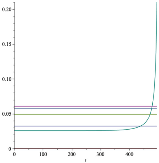
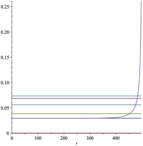
Suppose the expected return on the fund and the spending rate is . Here . Also suppose in some units. We consider .
In Figure 1 the horizontal line from represents the martingale where the spending rate is . The increasing curve represents the submartingale where the spending rate is , while the decreasing curve is the supermartingale where the spending rate is .
Figure 1.
Various expected developments of an endowment fund. Red = martingale, green = submartingale, light blue = supermartingale.
Here we can answer various types of questions. To illustrate, suppose we ask the question: How long does it take before the expected value of the fund is up ? The answer is years. Next, for the fund with , it takes years before the expected value is down .
We have proven the following result:
Theorem 3.
Suppose c is the spending rate of an endowment fund W and is the expected real rate of return on W. Then we have the following three situations:
(1) If , then is a submartingale and as
(2) If , then is a supermartingale and as
(3) If , then is a martingale and for
In the continuous-time model with Brownian motion driven uncertainty, for the corresponding martingale result it was shown that the wealth eventually converges to zero with probability 1 (Aase and Bjerksund 2021, p. 11). Here we can appeal to a theorem of Jean Ville (1939) in the context of a filtered probability space , suppose . If a nonnegative martingale diverges to infinity when E happens, then . This result does not need the iid assumption which, admittedly, is rather strong. Together with this assumption, however, with the results of the next section it says roughly the same as the continuous-time result: The martingale will approach 0 with probability 1.
5.2. Almost Sure Convergence
Let us move to convergence almost surely. Here we have the following result.
Theorem 4.
Let c be the spending rate and the rate of return of the endowment fund (a random variable). Then we have the following:
(a) If , then almost surely as .
(b) If , then grows without limit almost surely, as t increases.
The proof, which can be found in Appendix B, makes use of the strong law of large numbers (SLLN).
Suppose now that the spending rate is being used, as advocated by some researchers and spokespeople.3
In this situation
by Jensen’s inequality since the logarithmic function is strictly concave. Furthermore
since . By Theorem 4, part (a), it follows that with probability 1 as . By the above theory it also follows that as . From this we realize that this policy, that of spending the expected real rate of return, is not a viable spending rule for an endowment fund.
Let us consider the case (b) of the theorem,
This inequality holds if and only if the spending rate c satisfies
Let us define
It turns out that can be approximated by : By a Taylor series approximation of the logarithmic function we know that the standard approximation for financial return data for the term is . Also by a Taylor series approximation of the exponential function. The latter can be written , and this expression is seen to be well approximated by (to the fourth order of approximation in the examples we consider).
This means that is a threshold which an extraction rate c should not pass from below in order to have long term “viability” of the endowment fund.4
How accurate is this approximation, and is it on the conservative side? To check this, we need the probability distribution of . As a numerical illustration, suppose that and var. This means that .
To compute we the need the probability distribution of . As an illustration, let where is one-dimensional and discrete, taking two values and with , and , so that and , see Section 6.1 below for these values. Using this, we obtain . This means that , so the difference which is sufficiently small for most practical purposes and on the safe side. When the spending rate , this means that as well and the spending rate c passes the long run test.5
By construction it is always true that and . With this trivial, but important observation, we have the following reminder:
Corollary 1.
Let be the expected real rate of return of an endowment fund. Then we have the following:
If the spending rate is set equal to the expected real rate of return , then the fund value almost surely as , and the expected value as .
Notice that this result is independent of any of the preference parameters, it depends on our statistical assumptions only.
Also, under our conditions neither convergence in rth mean nor convergence almost surely implies the other (here ).6
Next we illustrate this result by numerical examples. Our results can be compared to the corresponding results for the time-continuous model, see Aase and Bjerksund (2021); here we present extensions.
As indicated, not all the consequences of the iid assumption are realistic. Still this is a standard assumption and give some rather explicit and also reasonable results. However, no fortunes will ever become infinite, a fact which will be addressed in Section 10, where we suggest to relax the iid assumption.
6. Numerical Illustrations—Expected Utility
For reasonable market quantities, we compare the optimal spending rate for an endowment fund to the real expected rate of return from the fund. The optimal spending rate we interpret as the consumption to wealth ratio of the previous section. We also compare to the thresholds of the last section, and to a quantity related to the certainty equivalent rate of return of the fund.
One reason why we do this is the claim that it is both optimal and sustainable to spend the expected real return of a sovereign fund. For example, and as mentioned, this is the rule, determined in parliament, for the Norwegian SWF Government Fund Global, one of the World’s largest sovereign funds. Based on the last section, our claim is that this is not an optimal spending rate, it is too high, and will, if followed, deplete the fund at a final future time with probability 1. We consider this fund as an example in Section 9.7
Here we illustrate the above theory by use of real market data. We assume the agent takes the US-market as given, where the risky part of our fund is represented by the S&P-500 index. This corresponds to one of the best functioning securities markets in the World, and should be representative in construction of the underlying market quantities. The data are as follows.
In Table 1 we provide the key summary statistics of the data in Mehra and Prescott (1985) on the real annual return data related to the S&P-500, denoted by S, as well as for the annualized consumption data, denoted c, and the return on Government bills, denoted b 8.

Table 1.
Key US-data for the time period 1889–1978. Discrete-time annual compounding.
Example 2.
Consider the above market data, and the following preference parameters: and .
For these parameters and with the market data of Table 1, the optimal portfolio fraction in the risky part of the market is , the expected rate of return on the fund is where and from the above table. Furthermore, , where M is defined in Equation (11), and the volatility of the return on the fund is , where all follow from the above table.
For reasons to become clear below, we consider the following expression
while the next quantity is the key for asymptotic comparisons, defined in Section 5,
We see that when , , and when , .
When the extraction rate is below , the fund grows in t with probability 1, while if it is above , the fund value converges to 0 with probability 1 as .
Normally we have that in which case , so may be a viable candidate for a spending rate. We will refer to this quantity as the certainty equivalent return in this paper (although this is standard terminology only when ).9
From the last section recall the interpretation of the threshold . For the above parameters the certainty equivalent rate of return , and . The optimal spending rate is . This value is seen to be consistent with long term sustainability of the fund. However, if the real rate of return () is used as the spending rate, this is not sustainable in the long run and the fund will converge to 0 almost surely as t goes to infinity. Moreover, will converge to 0 at a geometric rate as .
With a finite horizon of years, the extraction rate in Equation (14) is time dependent, and will increase sharply as the horizon comes closer. In Figure 2 we present a graph of the optimal extraction rate, and in the same graph we also represent the real rate of return together with m, and .
Figure 2.
The optimal extraction rate as a function of time (EU). green = , red = , light blue = m, light green = , blue = .
The hyperbolic type curve is the optimal extraction rate , the upper horizontal line is the expected rate of return on the fund, the next horizontal line is m, then follows , and the lowest horizontal line is the certainty equivalent rate of return . Also for any finite horizon T. The growth rate of the optimal consumption is with standard deviation .
Consider the following illustration: In Figure 3 we show five graphs as functions of for . The lowest one is the long term optimal spending rate as a function of , the next lowest is the certainty equivalent , then comes the threshold value , the next highest is the martingale threshold value and the highest located curve is the expected rate of return on the fund . These quantities are time independent, but will depend on via , since they depend on .
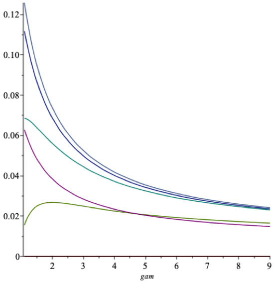
Figure 3.
The functions , , , and as vary. grey = , blue = , green = , red = , light green = .
We see that the long term optimal spending rate is lower than the other quantities for any reasonable value of the relative risk aversion . This illustrates our above claim in this example, and moreover it indicates that the criterion of spending the real expected rate of return is not only larger than the optimal one, but also larger than the two threshold values and for “any” values of and . This means that the fund will (1) converge to 0 with probability 1 with this extraction policy regardless of the relative risk aversion , and (2) the expected value of the fund will converge to zero as , with as the spending rate.
One question arises here: Does spending increase with the parameter , or does it decrease? With increasing relative risk aversion one would think that optimal spending decreases with the parameter. With increasing resistance to intertemporal substitution in consumption one would think that the optimal spending will increase with the parameter. The parameter is known to measure both these properties. In Figure 3 there seems to be a compromise: When the parameter is smaller than about 1 it has the resistance to consumption substitution property; when larger than 1 it seems to represent relative risk aversion. The resolution of this puzzle will be clear with recursive utility, where the two conflicting interpretations of this parameter have been separated into two different parameters.
6.1. Discrete State Probabilities
As mentioned in Appendix A, in order for a discrete time model to be complete, the set of states of the world must be finite. In the present situation we have one risky asset, the index, so let us for the following illustration use the simplest possible version for the with two states of nature, “up” and “down” with probabilities and respectively. In this situation the formula for the spending rate is the following
where u and d satisfy the two equations (i) and (ii) . We must estimate the up probability from return data in the stock market, and determine u and d from the two equations (i) and (ii). Consider the following estimates: and . This gives and . This is calibrated to give the same value of the spending rate for and as the above model based on truncation of Taylor series.
In Figure 4 we show the same graphs as in Figure 3, with the addition that the spending rate in Equation (19) is included together with the one from the previous figure. These two curves can be seen to be almost indistinguishable. It is noteworthy that the simple Binomial model is this flexible.
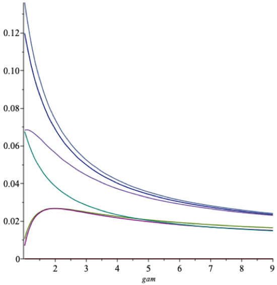
Figure 4.
The functions , , , and as vary. grey = , blue = , light red = , green = , red = .
6.2. Patience
What we mean by a reasonable patience factor is illustrated next. In Figure 5 we show graphs of , , and , as functions of . Here .
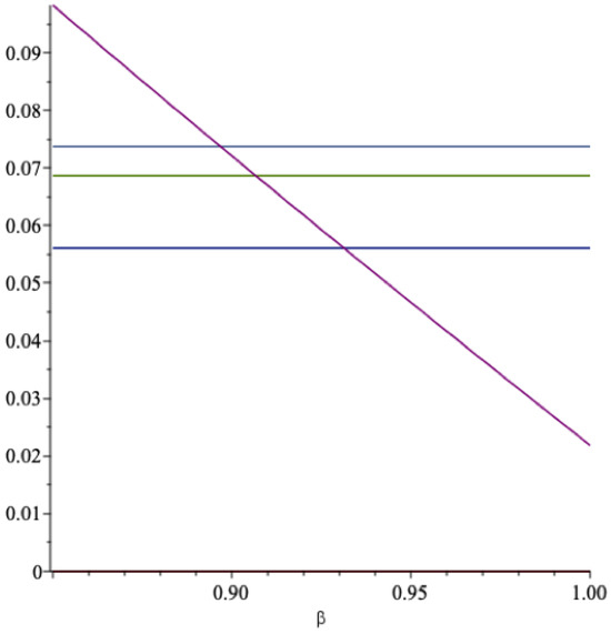
Figure 5.
The functions , , , as vary. red = , light blue = , light green = , blue = .
The falling (convex) curve is the optimal spending rate as a function of . The next horizontal lines are independent of , where the highest is the line showing the real rate of return on the fund, and the lowest one is the threshold for a.s. convergence, while the one in the middle is the -threshold. The figure shows that when the agent is impatient enough, the optimal spending rate is larger than the expected rate of return on the fund, then comes a range where is lower than but larger than m, and when the agent is patient enough, the optimal spending rate is lower than both m and . For this example we see that this happens when . Normally one sets in applied work. A nation as the agent must be considered patient.
In the expression for the parameter occurs together with the parameter as . When increases, so does . This has the effect that the agent appears as more “patient” with increasing as can be observed in Figure 3, where the optimal spending rate decreases as increases. This decrease is primarily a consequence of increasing risk aversion, but impatience and risk aversion are not completely disentangled in this model.
With the tools of the asymptotics section we can, for example, calculate how many years it will take before has deteriorated, or increased a certain fraction, depending on the spending policy (recall Figure 1). To illustrate, in this situation with an optimal spending rule and expected return on the fund , it takes about 12 years for to have increased using the optimal spending rule, while it takes about 61 years for to have decreased using as the spending rate.
7. Recursive Utility
Recursive utility (RU) is considered to be a more realistic representation of preferences than expected, additive and separable utility (EU) that we have considered so far. In particular RU separates risk aversion from consumption substitution in temporal models, which is important, since since these two properties are rather different. Recursive preferences have an axiomatic underpinning in the basic work in the field by Kreps and Porteus (1978).
Again we want to solve the problem (1), where the utility function is defined via the following “aggregator”
where v is a felicity index with inverse function , is a conditional certainty equivalent as of time t, and is the patience factor defined as as before. In this case in (1) is given by .
So, where does such an aggregator come from? The standard separable and additive expected utility representation has an ordinally equivalent version which, when normalized, can be expressed in recursive form. For example, the representation
is ordinally equivalent to the recursive version in (20), provided the conditional certainty equivalent is the one of expected utility with felicity index v.
Thus, in order to deviate, in a non-trivial way, from the standard, additive representation of preferences, it is assumed that the conditional certainty equivalent can be represented as above, but with a different felicity index u: , . This turns out to be an important step, since consumption substitution in a deterministic world is something very different from risk aversion, where the latter only makes sense under uncertainty. This essential difference is taken into account by the recursive model.
On the one hand this approach stays close enough to the standard, additive representation of preferences to still benefit from many of its useful properties, insights and interpretations, on the other this step is significant enough to avoid some of its unrealistic and negative features. However, this generalization comes at a price of added complexity, as is naturally the case with most generalizations.
In this article we employ the two standard functions v and u, defined up to affine transformations as and , with inverse functions and respectively. The following scale invariant aggregator results from (20)
where the conditional certainty equivalent m is given by
The parameter corresponds to the agent’s relative risk aversion in the standard one-period model (the time-less model), and has the same interpretation here. Similarly, in a deterministic setting the parameter , where is the elasticity of intertemporal substitution (EIS) in consumption. These parameters correspond to different properties of the individual’s preferences—and should be measured independently. In the standard, additive expected utility model, , which turns out to be rather restrictive.
When , the felicity index , and , and when , then we have , and .
The parameter is the ‘patience’ factor, where as for EU. The impatience rate .
While preferences over deterministic consumption plans are solely determined by the function v, the limitation of the expected additive, discounted utility in the presence of uncertainty rests on the fact that the function determining risk aversion also governs the purely deterministic development.
RU overcomes this latter problem, and other problems, by simply separating v from u.
The version in (22) is known as the Epstein-Zin aggregator (see Epstein and Zin 1989, 1991; Chew and Epstein 1991). For continuous-time see Duffie and Epstein (1992), and for risk premiums and the equilibrium interest rate see, for example, Aase (2016).
7.1. Optimal Consumption and Portfolio Selection with Recursive Utility
In Appendix C we have relegated the analysis of the recursive model, where we derive a closed form expression for the optimal consumption in Equation (A19), and compare it to the corresponding expression for EU. Moreover, we find the optimal portfolio selection rule, and show that this is the same as for the EU-model, assuming a deterministic investment opportunity set.
These two results are the basics for our expression for the optimal spending rule for RU, which follows next.
7.2. Optimal Consumption to Wealth Ratio (RU)
We now address the optimal spending problem of a sovereign wealth fund. Starting with the wealth Equation (A13) in Appendix C, we proceed as before with the expression in (A20) in Appendix C for the optimal consumption. We have the following result:
Theorem 5.
The connection between the optimal wealth and the optimal consumption at any time t is given by the following relationship:
The proof can be found in Appendix D.
In order to progress further, we need some simplifying assumptions. From now on we adopt the assumption of Section 3.2 of a stationary and deterministic investment opportunity set for all t. The same type of assumptions are made as in the case of the expected utility, from which we can characterize the conditional expectation on the right-hand side of Equation (23).
Recall that is the expected real rate of return on the wealth portfolio W, and is the corresponding variance of the return rate of the fund.
We use Taylor series approximations and neglect moments of order three and higher. This leads to the following result:
Theorem 6.
(a) Consider the finite horizon case . Define
Under the above assumptions the optimal consumption to wealth ratio can be written as follows:
(b) Consider the infinite horizon case where . The optimal consumption to wealth ratio is given by
provided .
The proof can be found in Appendix D.
Notice that the optimal spending rate depends on the statistical dependence between the state price and the return on the wealth portfolio via the term for .
Remark 3.
The optimal spending rate with recursive utility in continuous time with continuous price processes based on Brownian motion was presented in Aase and Bjerksund (2021). The exact expression for the spending rate is the following
again a convex combination of the impatience rate δ and the certainty equivalent rate of return from the fund. In the convex combination the parameter ρ now plays the role that γ played in the corresponding formula for expected utility.
As with EU-theory, we can demonstrate that the expected rate of return is strictly larger than the optimal spending rate with RU developed above. The simplest way to prove this, is to show that the discrete spending rule is well approximated by the one in continuous time, for which this is true. This is demonstrated below. From the expression (27), it follows that the expected rate of return is larger than the extraction rare whenever
Since the second term on the right-hand side is negative, this inequality remains true for reasonable values of the preference parameters. We formalize this as:
Proposition 2.
The expected real return on the fund is larger than the consumption to wealth ratio, the optimal extraction rate, that is
provided the agent is reasonably patient, i.e., β is large enough.
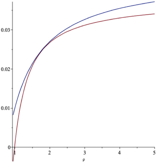
In Figure 6 we present a graph of the function in (27) together with the optimal extraction rate in Equation (26) as functions of ρ when and .
The lowest graph is the spending rate in Equation (27). The spending rate in Equation (26) is seen to deviate for more extreme values of ρ, where the approximation may not be as good as for more central values of this parameter.
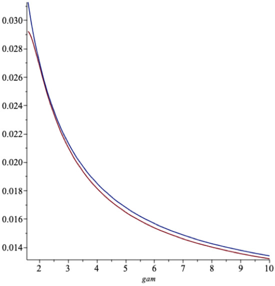
Next we compare these two spending rates as functions of γ when and (Figure 7).
The lowest graph is the one in Equation (26). The fit is seen to be reasonable, given γ is a bit larger than 1.
Below we also compare the continuous-time spending rate with the one based on the present discrete time model using the discrete state probabilities. The spending rate with RU and the Binomial version is the following:
For the recursive model we calibrate the discrete state version for , and to , , and using (26).
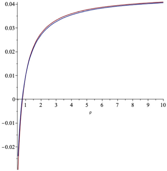
In Figure 8 we graph the spending rate in (27) and the Binomial one in (29) as functions of ρ when and :
Figure 8.
The cont.time and the Binomial spending rates as vary.
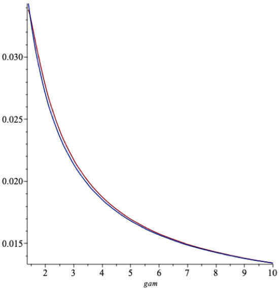
As we see, this fit is rather impressive. In Figure 9 we do the same comparison when γ vary for and .
Figure 9.
The cont.time and the Binomial spending rates as vary.
Also here the fit is excellent.
Notice the different shape of these curves: The optimal spending increases with the parameter (Figure 6 and Figure 8), and decreases with the parameter (Figure 7 and Figure 9). With EU there is only one parameter for these two different phenomena, so both these developments can not hold for EU. This we return to below.
7.3. The Conditional Expected Consumption Growth Rate and the Associated Volatility
With the techniques of Theorem 6, we can readily find the expected growth rate of the optimal consumption and its standard deviation. Let
The conditional expected consumption growth rate is
Also
From these two quantities we can find the standard deviation of the conditional expected consumption growth rate as
The proof can be found in Appendix D. By setting and we obtain the corresponding results for EU.
8. Numerical Illustrations—Recursive Utility
First consider the same data as in Example 2, with preference parameters , and . This parameter constellation represents preference for early resolution of uncertainty. Only the the optimal extraction rate function changes, while the other data remain the same as in Example 2. The long term optimal spending rate , which is comparable to the optimal value for EU in Example 2.
Next consider the following example.
Example 3.
Let , and . The optimal portfolio weight , representing a more risky portfolio than above, , , and , and . The optimal extraction rate in the long run is , while it is for the expected utility model. The graphs corresponding to Figure 2 are here (Figure 10):
Figure 10.
The optimal extraction rate as a function of time (RU). light red = , green = , red = m, grey = , light green = , blue = .
The upper line is the expected return on the fund, the next line corresponds to the threshold , then follows , and we notice that the optimal rate is below these two lines consistent with long term tests, while the certainty equivalent return rate is slightly above the optimal rate. The expected rate of return on the fund is seen to fail both the long term tests as a spending rate, in agreement with Corollary 1. The optimal spending rate , is the hyperbolic-type curve sharply increasing towards the horizon, which passes both long-run tests almost to the end of the horizon. The lowest line, tangent to this curve, is .
The growth rate of the optimal consumption is with standard deviation . Since , the agent has preference for late resolution of uncertainty.
When the parameter ρ decreases, the resistance to substitute consumption across time decreases and the optimal spending rate decreases. For example, when and the other parameters are as above, then . If the impatience increases, the optimal spending rate increases. For example, if , and , then for RU and for EU. The growth rate of is now with standard deviation . Impatience does in general not help much on growth.
In Figure 11 we show a graph of the optimal extraction rate as a function of for the values of and . Also included are from the top: the expected rate of return , then the two thresholds m and , explained Section 6, and the lowest line is the certainty equivalent return rate , all with the same numerical values as in Figure 10. These four quantities do not depend on . This follows, since the portfolio fractions only depends on the relative risk aversion also for RU, and the expected rate of return on the fund where is the vector of excess returns on the risky assets and r is the risk-free rate of return. Hence only depends on the preferences via the parameter also for recursive utility.
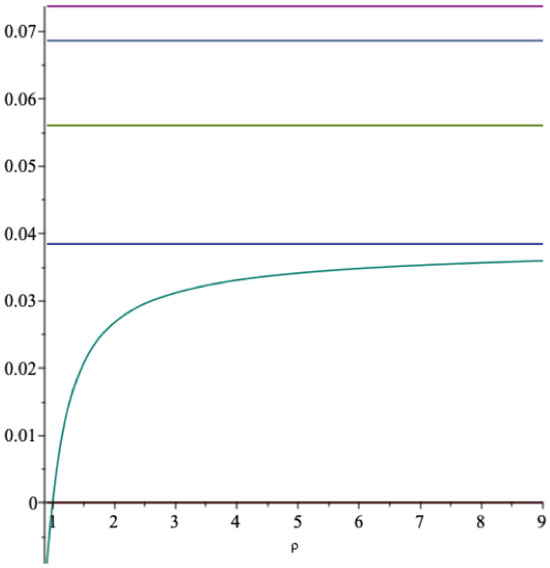
Figure 11.
The optimal long term spending rate as a function of . red = , grey = , light green = , blue = , green = .
The optimal spending is given by the the lowest curve increasing in the parameter . By increasing the parameter , optimal spending increases for all values of . This parameter measures the individuals relative degree of resistance to intertemporal substitution of consumption. With this interpretation in mind, it is quite natural that spending increases with . Notice that nothing dramatic happens when passes in value, where the agent moves from having preference for early resolution of uncertainty, to preference for late resolution. We observe again that the optimal spending rate passes both the long term tests with good margins.
For the truncated model the parameter can not be too small, since then the curve starts out increasing, reaches a maximum and then continues with a decreasing convex shape. When the agent becomes impatient enough, say , this may seemingly happen. However, this feature is not real: When we use the Binomial model this pattern disappears (see for example Figure 8), and the curve is strictly increasing as in Figure 11.
In Figure 12 we show the graphs of optimal spending rate as a function of , as well as the quantities , , and , when and . The lowest graph represents the optimal long term spending rate. Note that when increases, optimal spending falls, which is intuitive when this parameter is relative risk aversion. This is the opposite of what happens if increases in Figure 11, which is also intuitive with the interpretation of as .
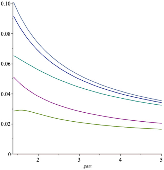
Figure 12.
, , , as functions of (RU). grey = , blue = , green = , red = , light green = .
For the case of EU, Figure 3 indicates that this problem is “resolved” by increasing spending for low values of , where it presumably can be interpreted as resistance to intertemporal substitution of consumption, while optimal spending falls for larger values of , when it has the interpretation of relative risk aversion.
That these two properties, relative risk aversion measured by the parameter and resistance to intertemporal substitution of consumption measured by the parameter , represent two very different features of a preference relation, is hardly better illustrated than this.
The highest falling curve is the expected rate of return on the fund, the next curve is the martingale threshold , then the graph and finally the curve representing the certainty equivalent .
The optimal spending rate is seen to pass both the long run criteria for all vales of with good margin, while the expected rate of return on the fund fails both, in agreement with Corollary 1.
When the parameter is close enough to 1, the spending curve is large, which is due to the singularity in the coefficients a and b at . In this case the truncations are not valid (but the discrete state probability version is not similarly affected).
For the data of this section and with an optimal spending rule with recursive utility and expected return on the fund , it takes about 12 years for to have increased using the optimal spending rule, while it takes about 41 years for to have decreased using as spending rule.
These examples and graphical illustrations tell us that the models, both of the and of the type, are fairly robust with respect to the size of the optimal spending rate. By changing the preference parameters within reasonable ranges, the optimal rate changes only moderately. This means that our results should have real world policy implications regarding optimal spending rates from endowment funds.
From Corollary 1 it follows that the spending rate can not be set equal to the expected real rate of the fund. This result is independent of all the preference parameters.
We round off with the case of the Norwegian SWT Government Fund Global.
9. The Norwegian SWF Government Fund Global
For this sovereign fund the Norwegian Ministry of Finance set down a commission in 2016 to consider the asset allocation problem. Table 2 below reflects the commission’s market view on equity and risky bonds.10
Table 2.
The commission’s market view, Norwegian Ministry of Finance (2016).
The commission recommends an equity share of . Given a riskless rate of and an equity premium with expectation and standard deviation , the excess return , , the market-price-of-risk , and .
This translates into an implicit relative risk aversion of . This implies that the expected real rate of return and the standard deviation .
The certainty equivalent fund return is , and . Observe that is larger than both and m, thus not acceptable in the long run (with probability 1 and in 1th mean).
Let . Then the optimal long term spending rate with expected utility is , which passes both the long run tests. This is lower than the expected real return on the fund.
With recursive utility, assuming and , where the other parameters are as above, then and we have preference for late resolution of uncertainty. When we have , preference for early resolution of uncertainty, and the optimal long term spending is , assuming the other parameters are as above.
For the data of this section and with an optimal spending rule with recursive utility and expected return on the fund , it takes about 12 years for to have increased using the optimal spending rule, while it takes about 40 years for to have decreased using as spending rule.
At the end of 2021 the market value of this fund was 1299 billions USD, and decrease in 22 years amounts to 65 billions USD in expectation. If the optimal spending rule had been used, the fund would have been billions USD higher in expectation after 40 years. Should the young generations of Norwegians accept this?11
In Figure 13 we illustrate the optimal long term spending rate as a function of the parameter . The parameter and . The upper line represents the expected rate of return on the fund . The next line is , then follows , and finally . The optimal spending rate is the lowest increasing curve, and passes both the long run tests. In contrast, the expected rate of return on the fund, as a spending rate, does not pass either test (recall Corollary 1).
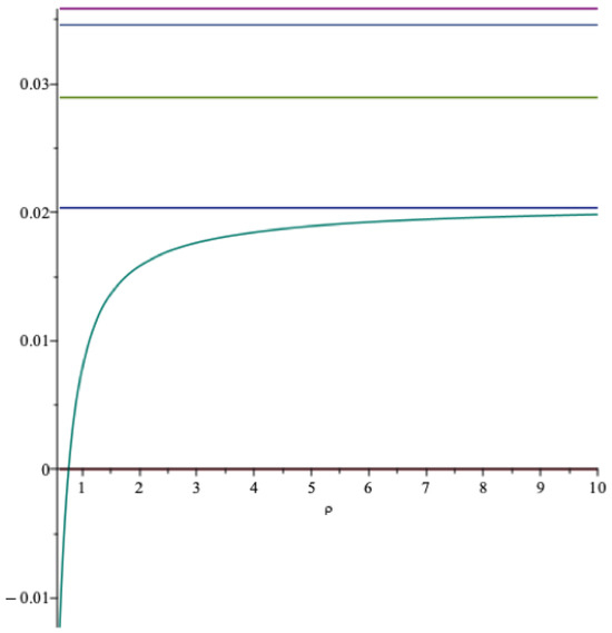
Figure 13.
The optimal spending rate as a function of . red = , light blue = , light green = , blue = , green = .
Let us illustrate with some concrete values of . In Figure 14 the parameter , and as above, where the horizon is years. This implies preference for early resolution of uncertainty. We have the following picture in Figure 14: The three upper horizontal lines have the same ranking as in the previous figure ( and are the same), the quantity is not shown, and the lowest horizontal line is the optimal long run extraction rate .
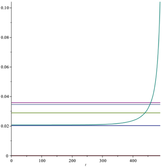
Figure 14.
The optimal extraction rate as a function of time (RU). red = , grey = m, light green = , green = , blue = .
This latter rate, here for RU, is larger than indicated in the previous figure, since the impatience rate has increased. The hyperbolic type curve is the optimal extraction rate . This rate passes all the tests up up to around 400 years. In this example the growth rate of the optimal consumption is with a standard deviation of . The optimal long run spending rate with EU is here .
Next we let vary: This corresponds to different values of the portfolio weight , which would fall from to when increase from to 5, following a convex, hyperbolic curve. For and , Figure 15 gives a graph of the optimal long term spending as a function of , the lowest curve in the figure.
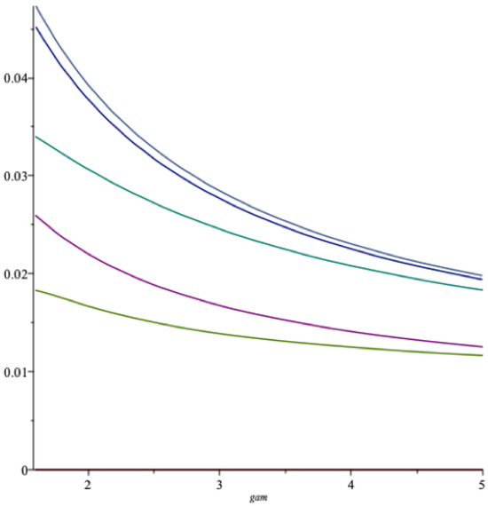
Figure 15.
The optimal spending rate as a function of (RU). grey = , blue = , green = , red = , light green = .
In Figure 15 is also included from the top; the expected rate of return, the martingale threshold m, the threshold and the certainty equivalent , all as functions of . Higher risk aversion leads to a lower optimal spending rate.
Notice again the striking difference between the shapes of the optimal spending as functions of in Figure 13 and in Figure 15: Intertemporal substitution of consumption is both qualitatively and quantitatively very different from relative risk aversion.
What if the optimal rate becomes very low or even negative? Suppose corresponding to , and so the agent is patient. Now the optimal long term spending rate is for recursive utility, i.e., negative. This must clearly be ruled out in the infinite horizon case, but still makes sense with a finite horizon. Say for instance that the fixed horizon is years from now. Does this mean no spending at all?
Clearly not. See Figure 16, where the three upper horizontal lines have the same ranking as in Figure 14, then follows and the lowest line is . Note that in this case there is a gap at so that .
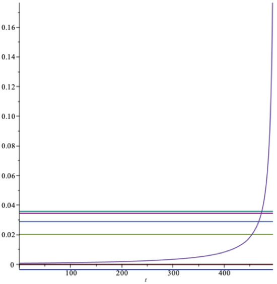
Figure 16.
The optimal spending rate as a function of time (RU). grey = , red = m, light blue = , green = , light red = , blue = .
The optimal spending the first year is of the fund value, the optimal spending in year 30 is , the optimal spending in year 70 is , in year 100 it is , in year 450 it is and in year 473 is is of the fund value, which is equal to the expected real rate of return on the fund in this situation, and so forth. When the parameter decreases further, the optimal spending rate decreases, the gap widens, and still the optimal spending with a finite horizon is strictly positive, and increasing as the horizon comes closer.
Provided , where here, the fund grows with probability one as t increases. (For other parameter values, if the fund value converges to 0 almost surely).
The consumption growth rate in this example is with a standard deviation of .
In this example consumption substitution dominates.
Exogenous Income Streams
Suppose there is an exogenous income stream added to the fund each year. The consequences of this will now be discussed. Let us assume that is added to the fund in year t, where this stream of cash flows are assumed iid. We assume the amount at time t is invested in the financial markets together with the rest of the fund , where the new fund is denoted and the new spending we call . Under this assumption the real expected return is equal to , since there is no reason that this addition to the fund will alter the expected return so long as the same optimal portfolio selection rule is used on the total. Recall that and , that is, both these key parameters depend on market related quantities only. This means that the threshold values and are the same as before, and so is .
What about the optimal spending rate ? For expected utility we notice from the proof of Theorem 1 that the basic change happens in the budget constraint, where the Lagrange multiplier obtains a new value, but from the proof this is seen to have no consequence for the consumption to wealth ratio . For recursive utility we see from the proof of Theorem 5 that the optimal spending rate depends in addition to the budget constraint, also on the parameters and , which we have argued do not change by the added income stream. Accordingly, the spending rate and the final horizon version will both remain unchanged by I for both types of preferences.
However, optimal spending will naturally change, that is, increase, since we assume . This follows since the optimal spending with an exogenous income stream is still proportional to wealth:
where is the optimal spending with no added income stream.
For the Norwegian SWF Government Fund Global this is of interest, since still an exogenous addition to the fund occurs each year. As explained, this will allow a larger spending, but the optimal “fiscal” rule, that is, the consumption to wealth ratio, remains unchanged by income I.
As an example, for the year 2021 the market value of this fund was billion NOK, where the addition () from the external oil-related activity was billion NOK. This amount has been stable for several years, supporting our iid assumption. Supposing the optimal spending rule was this year, this would amount to 188 billion NOK from the fund ex the direct oil supplement, and in addition 59 billion NOK from the latter.
10. More General Asymptotics
In applied works, like this paper, one should recall that the aggregate wealth in the World is finite, and will remain finite in the future as well. In our analysis in Section 5 the iid assumption on returns led to violations of this fact. In order to take this observation into account, we now relax the iid assumption. We also allow the spending each year to depend on the information at time t, instead of being constant across time. The spending decision is now taken, adaptively, each year at time t, when the real return on the fund the next year, is still unknown, but its probability distribution is known. Moreover this return is not supposed to have the same probability distribution every year but can vary across time. For our first analysis we do not need the returns to be independent either. See, for example, Lo and MacKinlay (2011) for support on these assumptions.
Starting with
we recall that is a submartingale provided a.s. for all . Here this means that as long as for all t, is a strict submartingale, while equality give the martingale property and the reverse inequality means that the wealth process is a strict supermartingale.
The following result is called the Martingale Convergence Theorem (MCT) (see, for example, Breiman 1968, Th. 5.14, p. 89):
Theorem 7.
Let be a submartingale such that , then there exists a random variable such that a.s. as and
We claim that the assumption of the MCT is both realistic and also technically feasible in our model since we have dropped the assumption that the real returns have the same distributions across time. We therefore make this assumption for our wealth process .
This theorem has an analogue for supermartingales, where the above limsup assumption is for the negative part of . Since the wealth processes are non-negative, this assumption becomes void here. In this situation there exists a random variable such that the supermartingale converges to a.s. and . In this case this limiting random variable will not be equal to zero a.s.
A process is uniformly integrable if for all t and moreover . We have the following result (e.g., Breiman 1968, Proposition 5.19, p. 91):
Theorem 8.
If is uniformly integrable, then . If a.s., then , and .
Suppose our wealth process is uniformly integrable as well. From the MCT it follows that a.s., in which case we obtain that from Theorem 8, provided the adaptive spending rule , satisfies the criterion , for all t.
This means that our previous theory with two different thresholds m and for 1tst mean convergence and convergence almost surely, respectively, simplifies to a theory with one single threshold that apply to both forms of convergence and which leads to the same limiting random variable .
The analogous result for supermartingales says that the wealth converges to a random variable both almost surely and in 1st mean; again our two previous thresholds reduce to a single one, valid for both types of convergence. Spending the real rate of return falls in this category.
Under our conditions we can also say something about the probability distributions of the limiting random variables. Let us retain the assumption about different probability distributions for the real returns, but here we assume independence. First, since the wealths converge a.s., they also converge in probability, and this in turn implies converge in law, that is, in distribution (Tucker 1967, Th 6, p. 105). Consider the following transformation of the wealths
Let us first restrict attention to the submartingale case where for all t. Here the are all constants.
Since ln is a continuous function, it follows that ln converges in probability (Tucker 1967, Th 5, p. 104), and hence in law as well. By the independence assumption one would, perhaps, conjecture that the limiting distribution is normal, but since the the return distributions differ across time, this is not guaranteed. Here we may use a Lindeberg-Feller type central limit theorem, see Feller (1966), Ch. XV, p. 518, where an additional condition regarding variances is shown to be sufficient for normality. Assuming we have a normal limit in the log version (32), that is ln is normally distributed, via convergence in probability again (the function is continuous), we obtain that converges in distribution to a lognormally distributed random variable ,12, that is exp is lognormally distributed by definition.
A similar result also holds for the limiting random variable , showing that this random variable is, under these conditions, not identically zero in the supermartingale case. It has a much smaller expectation than , and a smaller variance as well (see Appendix E).
Under the assumptions of the Lindeberg-Feller theorem, the limiting random wealth dominates in first order stochastic dominance (FSD), that is, all agents with nondecreasing utility functions (at the horizon) prefer to . As a consequence, all owners of wealth funds, as long as they prefer more to less, will prefer to . The details can be found in Appendix E.
The random wealth can, perhaps, be interpreted to represent what is meant by “the fund will last forever”. The optimal spending defined in Section 2 takes all periods in into account, with utility function defined in (2). The preferred temporal spending rule for satisfy the requirements leading to (modulo the equal distribution assumption).
This last section could be of interest for future research, where the results could be expanded and combined with empirical research on asset prices.
11. Summary
A central part of this paper has been to derive the optimal spending of an endowment fund, the consumption to wealth ratio. We show that this rate can not equal the expected real rate of the fund, since this would not be consistent with preference for diversification.
The rationale for this is that provided the fund is managed by diversification, this means that risk aversion, consumption substitution and impatience are essential in the optimal consumption and portfolio choice problem. To be consistent, the spending rate must also reflect this. As a consequence, the expected real rate of return is typically not an optimal spending rate, since this criterion is linked to risk neutrality.
We have developed two tests, with the property that if the optimal spending rate is below the corresponding threshold values, the fund will last “forever”.
For this purpose, we adopted, and further developed the life cycle model to fit our purposes, where we consider both expected additive and separable utility as well as recursive utility in the setting of discrete time.
We demonstrate that when the agent is reasonably patient, the optimal consumption to wealth ratio passes the two long run tests and is strictly smaller than the expected rate of return on the fund. If the spending rate is set equal to the latter, both tests are demonstrated to fail. Furthermore, for this spending rule and relaxing the conditions for convergence, the implications are that the fund converges almost surely and in expectation to a fund with low expected value. Spending below the single threshold that results for this kind of asymptotics, the fund is demonstrate to have a much better long term development: All agents who prefer more to less (a rather large group of individuals), will prefer the results of the optimal strategy to the fund values resulting from spending the real rate of return.
Our analysis clearly illustrated the advantage of considering recursive utility instead of expected utility. By separating intertemporal consumption substitution from risk aversion we obtained a much clearer picture of the properties of the optimal spending rate than provided by the the model based on expected utility.
Funding
This research received no external funding.
Institutional Review Board Statement
Not applicable.
Informed Consent Statement
Not applicable.
Data Availability Statement
No new data were created or analyzed in this study. Data sharing is not applicable to this article.
Conflicts of Interest
The authors declare no conflicts of interest.
Appendix A
Appendix A.1. The Financial Market
We consider a consumer who has access to a securities market, as well as a credit market. The security market consists of N risky and one risk-free security. The language and notation used here extends to continuous-time settings with a Brownian filtration. More details can be found in e.g., Skiadas (2009). The continuous-time analogue can be found in e.g., Duffie (2001).
The information filtration is generated by a d-dimensional martingale , where prime means transpose, such that
for , where , and . Any martingale M can be uniquely expressed as for some predictable process . We shall assume that the number of risky assets , where d is the spanning number of the filtration , and T is the finite horizon of the economy. The vector stochastic process B is a dynamic orthonormal basis for the set of zero-mean martingales.
The Doob decomposition of any adapted stochastic process is here a discrete-time, stochastic process that can be uniquely written as
or
for and predictable processes, which can be expressed as
Price processes are denoted by S, and when adjusted for dividends they are called adjusted price process, or gains processes, denoted by X. The price process S of any risky asset is assumed nonzero at nonterminal nodes, and the return process R is defined by
where is a -vector at each time t related to each single asset n, . By summing this equation over t we obtain what is called the cumulative return process ( is assumed to be arbitrary).
The securities market can now be described by the vector of expected returns of the N given risky securities in excess of the risk-less instantaneous return , and is an matrix associated to the risky asset prices, normalized by the asset process, so that is the covariance matrix for asset returns. Both and are assumed to be adaptive, measurable stochastic processes.
There is an underlying probability space and an increasing information filtration generated by the d-dimensional orthonormal basis B. The parameter , so that is the risk-free interest rate (also a stochastic process). The state price is connected to a density process given by
The process is called the market-price-of-risk process. The process can be interpreted as a conditional density process of a probability measure Q equivalent to the given measure P. In our framework is connected to the state price as follows, , where is the price of the risk-less asset, with simple return , so that . Here is the return on the risk-less asset in the time interval between and t, so it is -measurable. From this, using (A2), we obtain the expression
We consider discounted price process . The market-price-of-risk satisfies, for each cumulative return process , the equations
for each t, where is . Alternatively, satisfies the following system of equations
where the nth component of equals , the excess, conditional expected rate of return on security n at time t, . In (A4) is a matrix at each time t, assumed to be invertible (). The matrix is the covariance matrix of the risky assets in units of prices at each time t, where for short, with a similar notational simplification for .
Equation (A4) are the basic no-arbitrage restrictions for the financial market; when this system of equations hold, there exists a unique vector for each t, modulo some technical conditions. We then think of the market as being in a ‘dynamic equilibrium’, where a price taker, our consumer, trades optimally resulting in an optimal consumption plan c and generating optimal wealth W.
Having determined the market-prices-of-risk from (A4), these in turn determine the state prices in (A3). The vector gives a relationship between “risk” (conditional variances and covariances) and excess returns that must hold for there to be no arbitrage possibilities in the market, which is the basic message found in Black and Scholes’ (1973) theory.
Let be a trading strategy, which finances the consumption plan c and generates the wealth W. Let
where is the vector of portfolio ratios in the N risky assets. At the beginning of period t, the agent allocates the proportion of the wealth to immediate consumption and invests the remaining amount in the assets, with proportion going to asset and the remaining proportion going to the risk-less asset.
The end-of-period wealth is the result of this investment/consumption strategy and given by
where are the (simple) returns on the N risky assets, and is the (simple) return on the risk-free asset.
The consumer’s problem is, for each initial wealth level w, to solve
subject to an intertemporal budget constraint
The simple return on the wealth portfolio is given by the relationship
since consumption c is contained in W, where c may be interpreted as “dividend”.
The present problem is known as a temporal problem of choice.
Appendix B
Proof of Theorem 1.
Proof of Theorem 2.
We use the result of Theorem 1, and first we compute the following expectation:
where we have used independence across time of the random variables ,
At this point we use a Taylor series approximations to the second order of the power function , which gives for
This means that Equation (A8) can be written
As a consequence, from Theorem 1 the optimal wealth to consumption ratio, , can be expressed as follows:
The right hand side can be seen to be a geometric sum, which is given by the formula of the Theorem. Letting , this formula results in
provided the term . For reasonable values of the parameters this inequality obviously holds true, which proves the theorem. □
Proof of the Spending Formula (15) in Remark 1.
We start with the optimal spending formula in Theorem 2, which can be approximated as
and rewritten as
Next we use a first order Taylor approximation of the two last logarithmic functions, which results in
Finally, we use a first order Taylor approximation of the exponential function, which reduces the formula to the following expression
where . This is the formula in Remark 1. □
Demonstration of the Formula (16) in Remark 2.
Here we make use of the formula (15) in Remark 1. We want to show that
From our results in Section 3.2, this is the same as
Since and are close, this inequality can be written
Because and with good margin, this inequality holds true, with good margin, unless the impatience rate is too large. From Remarks 1 and 2 this also verifies Proposition 1. □
Proof of Theorem 4.
Starting with the relationship
where c is a spending rate, we obtain the following
With our iid assumption for it follows by the SLLN that
This means that
or
This shows that when then , which implies that grows without limit, almost surely, as t increases. This proves (b) of the theorem.
When the term on the other hand, then , which implies that almost surely, which proves (a). □
Appendix C
Appendix C.1. The First Order Conditions for Optimal Consumption: Recursive Utility
First we determine the optimal consumption. The agent is characterized by a utility function U and an endowment process . The agent’s problem is
where L is the space of adapted consumption processes, its positive cone, and is the state price deflator.
The Lagrangian of the problem is
where is the Lagrangian multiplier. Assuming U to be continuously differentiable, the gradient of U at c in the direction x is denoted by . This directional derivative is a linear functional, and by the Riesz Representation Theorem and for example, dominated convergence, it is given by
Here y is the Riesz representation of . The first-order condition is
This is equivalent to
This implies that for all .
Our next task is to characterize the Riesz representation y of U. When this is done, by the above result we have the marginal rates of substitution in the economy equal to the price ratios, .
Appendix C.2. The Marginal Rate of Substitution
In order to find the optimal consumption we need to find the Riesz representation p associated with the utility function U as explained in the last section.
Using directional derivatives and backward induction, we can show that the utility gradient is given by the following expression
from which it follows that the Riesz representation is given as
for , (see e.g., Aase 2021).
The intertemporal marginal rate of substitution, or the stochastic discount factor, is given by the formula
Along the optimal consumption path , that is, equals the price ratio.
In order to find a formula for the stochastic discount factor we must compute the quantities in (A11), which are
and
This means that the stochastic discount factor takes the form
Let c signify optimal consumption, and is the agent’s wealth at time t, given by
Our definition of wealth includes current consumption (dividend), so the simple real rate of return on the wealth portfolio over the period is given by
as before. By the definition in (A14), it now follows by a string of manipulations that
This expression has been the starting point for much of the literature on RU in discrete time models; see for example, Mehra and Donaldson (2008) and Cochrane (2008). This is the stochastic discount factor, first derived by Epstein and Zin (1989, 1991) in their seminal papers based on dynamic programming techniques.
We finally find the optimal consumption as follows: Below we assume and . Using that , we obtain from the relationship in (A15) that
It is instructive to compare this relationship to the corresponding one for expected utility, which is
Both these difference equations can be solved, using iteration and the properties of the logarithm. Starting with Equation (A16), it can be written
where is the expected simple return of the wealth portfolio at time s and is the corresponding vector of volatilities. Using this recursive relation also for and iterating, we obtain the following closed form solution for the optimal consumption
while the corresponding solution for the conventional EU-model is
This last expressions is equivalent to (8) in Section 3.1, and has been used in the analysis of the EU model, see Appendix A. Notice that and , where , r and are market related quantities and where are the optimal portfolio ratios, to be found in the next section for RU.
Appendix C.3. Optimal Portfolio Selection with RU
Let us consider the basic problem (1) at time t, where the optimal consumption has been inserted. Since the utility function is increasing, the constraint is binding and what remains is to solve the finite dimensional problem
Since the portfolio weights for the next period only appear in the second term of the aggregator f, the first order condition is
where we have used one of the formulas appearing after Equation (A11). Now we employ the property of scale invariance, which here means that . With this, the above can be written
Using the equation for the wealth dynamics in (A6), the first order conditions for are
for 13 In our case . With a deterministic investment opportunity set it follows that is deterministic, since the consumption to wealth ratio is deterministic. This means that we obtain the same first order conditions as for expected utility given in Equation (10), and under the same conditions is given by the Formula (11) also for recursive utility. This agrees with Skiadas (2009). A continuous-time version can be found in Svensson (1989).
Having solved the optimal consumption and portfolio selection problem in the life cycle model for recursive utility, the solution can be used to find the optimal spending rate, which we do in the next section.
Appendix D
Proof of Theorem 5.
Proof of Theorem 6.
We use the result of Theorem 5. We simplify the notation as follows in the first steps below:
First we need to compute expectations of the following type:
for . By use of a Taylor series approximation to the second order, we obtain
Here we have carried out the multiplication, then ignored terms of order 3 and larger, and used the property of in (A1).
We now apply the result of Theorem 5. By independence through time this gives that the reciprocal of the optimal spending rate, , can be written
where
This proves Theorem 6. □
Derivation of the Expected Consumption Growth Rate and Its SD for RU.
In this kind of analysis it can be of interest to find the expected consumption growth rate and the corresponding volatility. Here this can be done with the technique developed in the previous theorem. We start with the Equation (A18) from Appendix C.2, which can be written:
Following the steps in the proof of Theorem 6, the conditional expected consumption growth rate is
Next we need the conditional expected value of the following ratio
which is
From these two quantities we can find the conditional standard deviation of the expected consumption growth rate as
□
Appendix E
More General Asymptotics: The Distributions of W + and W -
Here we derive the distributional results for the two limiting random variables and of Section 10.
Starting with Equation (32), let us rewrite this as
where , s = 0, 1, 2, …, t. The variables have zero expectations and thus satisfy the Lindeberg-Feller (L-F) condition.
Let var, for , and , t = 0, 1, …
Under the conditions of the L-F theorem, it follows that the distribution of the random variable ln tends to the normal distribution , where and , assuming the two last series converge. That the first converge follows from the assumption behind the SCT.
Under the submartingale condition where , we have that so that ln for all , which shows that for all t, and . A consequence of this is that the mean of the limiting normal distribution, (ln, is large for large t.
The variance var, which does not depend on the constants .
From the connection between the two first moments of the normal and the lognormal distributions, it follows that the limiting random variable is lognormal with mean and variance . Here the variance depends on the constants via the term .
From this we notice that the mean of is large since is large, among other things.
Moving to the variable in the supermartingale situation, we first notice that since , we have that so that ln for all , which shows that for all t and . A consequence of this is that the mean of the limiting normal distribution, (ln, is small for large t compared to (ln. Notice that this is the situation if is used as the yearly spending rate.
Finally when moving to the corresponding lognormally distributed, limiting random wealth, we notice that is lognormal with mean and variance .
From this we notice that the mean of is much smaller than the mean of since is small (large in absolute value), among other things.
In particular this shows that , where the difference is large for large t as claimed. Moreover the above formulas show that variances satisfy as claimed in Section 10.
Finally regarding FSD, let and be the cumulative distribution functions of ln and ln respectively. These are both normally distributed, where the probability distributions are completely determined by their moments. We must show that for all .
Let U be standard normal . With this we have to show that , for all x, which is obvious since . This shows that ln dominates ln in the sense of first order stochastic dominance (FSD).
The lognormal distribution is not determined by its moments, but still this order also holds for the lognormal limiting random variables as well. To prove this we also go via the standard normal random variable U: We can write and analogously for . Using this, we find that for all x, which also follows from the inequality .
Accordingly, we have shown, as claimed, that dominates in FSD.
Notes
| 1 | A better notation for this parameter could be, say , where the parameter has both the above interpretations (if at all possible). |
| 2 | Also, the process is not uniformly integrable. An analogous situation occurs in the continuous time model with the geometric Brownian motion process. |
| 3 | Recall, this is the extraction rule for the Norwegian SWF Government Fund Global, determined by the Norwegian Parliament (Stortinget). |
| 4 | This rule is close to the one of Dybvig and Qin (2019) mentioned in the introduction, but not identical. |
| 5 | The standard approximation for is , which is here . Using the latter, we obtain . |
| 6 | Under the conditions of Section 10 this will be different. |
| 7 | We assume the fund is fully funded, so that the external influx to the fund has come to an end. When this is not the case, see Section 11. |
| 8 | There are of course newer data by now, but these retain the same basic features. |
| 9 | The Arrow-Pratt approximation to the certainty equivalent rate of return is given by when , a slightly larger quantity than . |
| 10 | The report, which uses geometric returns, i.e., , is referred in our list of references. This is translated to simple returns in Table 2. The covariance reported in the table stems from the following calculation , where the intertemporal correlation coefficient is . |
| 11 | In Norwegian kroner the amounts are, with the exchange rate of NOK to the USD: Fund value at the end of 2021: billions NOK, the decline in expectation is 614 billions NOK in 40 years, and the difference between the two spending rules amounts to billions NOK in expectation. |
| 12 | This was observed by Galton (1879) in a different setting. |
| 13 | Existence and uniqueness of this problem has been proved by Skiadas (2009). |
References
- Aase, Knut Kristian. 2016. Recursive utility using the stochastic maximum principle. Quantitative Economics 7: 859–87. [Google Scholar] [CrossRef]
- Aase, Knut Kristian. 2017. Economics of uncertainty and time: Optimal consumption and portfolio choice with recursive utility. In Finance in Society. An Anthology in Honour of Thore Johnsen. Edited by Mette Bjørndal, Frøystein Gjesdal and Aksel Mjøs. Boston: Cappelen Damm Akademisk, pp. 212–25. [Google Scholar]
- Aase, Knut Kristian. 2021. Elements of Economics of Uncertainty and Time with Recursive Utility. Wiley StatsRef: Statistics Reference Online 2021. Oxford: John Wiley & Sons, Ltd. [Google Scholar]
- Aase, Knut K., and Petter Bjerksund. 2021. The optimal spending rate versus the expected real return of a sovereign wealth fund. Journal of Risk and Financial Management 14: 425. [Google Scholar] [CrossRef]
- Black, Fischer, and Myron Scholes. 1973. The pricing of options and corporate liabilities. Journal of Political Economy 81: 637–54. [Google Scholar] [CrossRef]
- Blanchard, Olivier J. 1985. Debt, deficits, and finite horizons. Journal of Political Economy 93: 223–47. [Google Scholar] [CrossRef]
- Borch, Karl. 1960. The safety loading of reinsurance premiums. Skandinavisk Aktuarietidsskrift, 163–84. [Google Scholar] [CrossRef]
- Borch, Karl. 1962. Equilibrium in a reinsurance market. Econometrica 30: 424–44. [Google Scholar] [CrossRef]
- Breiman, Leo. 1968. Probability. Reading: Addison-Wesley. [Google Scholar]
- Campbell, John. 2012. Investing and Spending: The twin challenges of university endowment management. Paper presented at the Forum for the Future of Higher Education Symposium, Aspen, CO, USA, June 8. [Google Scholar]
- Campbell, John Y., and Ian Martin. 2022. Sustainability in a Risky World. Cambridge: Harvard University and NBER, and London School of Economics. [Google Scholar]
- Campbell, John Y., and Roman Sigalov. 2020. Portfolio Choice with Sustainable Spending: A Model of Reaching for Yield. Unpublished paper, Department of Economics, Harvard University. Available online: https://scholar.harvard.edu/campbell/publications/portfolio-choice-sustainable-spending-model-reaching-yield (accessed on 22 July 2024).
- Chew, Soo H., and Larry Epstein. 1991. Recursive utility under uncertainty. In Equilibrium Theory in Infinite Dimensional Spaces. Studies in Economic Theory. Edited by M. Ali Khan and Nicholas C. Yannelis. Berlin, Heidelberg, New York, London, Paris, Tokyo, Hong Kong, Barcelona and Budapest: Springer, pp. 352–69. [Google Scholar]
- Cochrane, John H. 2008. Financial markets and the real economy. In Handbook of Equity Risk Premium. Edited by Rajnish Mehra. Amsterdam: Elsevier. [Google Scholar]
- Cox, John C., and Mark Rubinstein. 1985. Options Markets. Englewood Cliffs: Prentice-Hall, Inc. [Google Scholar]
- Duffie, Darrell. 2001. Dynamic Asset Pricing Theory, 3rd ed. Princeton and Oxford: Princeton University Press. [Google Scholar]
- Duffie, Darrell, and Larry Epstein. 1992. Stochastic differential utility. Econometrica 60: 353–94. [Google Scholar] [CrossRef]
- Dybvig, Philip H., and Zhenjiang Qin. 2019. How to Squander Your Endowment: Pitfalls and Remedies. Unpublished paper, Washington University in St. Louis and University of Macao. Available online: http://dybfin.wustl.edu/research/papers/squander190217.pdf (accessed on 22 July 2024).
- Eeckhoudt, Louis, Christian Gollier, and Harris Schlesinger. 2005. Economic and Financial Decisions under Risk. Princeton and Oxford: Princeton University Press. [Google Scholar]
- Epstein, Larry, and Stanley Zin. 1989. Substitution, risk aversion, and the temporal behavior of consumption and asset returns: A theoretical framework. Econometrica 57: 937–69. [Google Scholar] [CrossRef]
- Epstein, Larry, and Stanley Zin. 1991. Substitution, risk aversion, and the temporal behavior of consumption and asset returns: An empirical analysis. Journal of Political Economy 99: 263–86. [Google Scholar] [CrossRef]
- Feller, William. 1966. An Introduction to Probability Theory and its Applications, 2nd ed. New York, London, Sydney and Toronto: John Wiley & Sons, Inc., vol. II. [Google Scholar]
- Galton, Francis. 1879. Gentic Images. Nineteenth Century 6: 157–69. [Google Scholar]
- Koopmans, Tjalling C. 1960. Stationary ordinal utility and impatience. Economctrica 28: 287–309. [Google Scholar] [CrossRef]
- Kreps, David, and Evan Porteus. 1978. Temporal resolution of uncertainty and dynamic choice theory. Econometrica 46: 185–200. [Google Scholar] [CrossRef]
- Lo, Andrew W., and A. Craig MacKinlay. 2011. A Non-Random Walk Down Wall Street. Princeton: Princeton University Press. [Google Scholar]
- Mehra, Rajnish, and Edward C. Prescott. 1985. The equity premium: A puzzle. Journal of Monetary Economics 22: 133–36. [Google Scholar] [CrossRef]
- Mehra, Rajnish, and John Donaldson. 2008. Risk-based explanations of the equity premium. In Handbook of Equity Risk Premium. Edited by Rajnish Mehra. Amsterdam: Elsevier, Chp. 2. pp. 37–99. [Google Scholar]
- Merton, Robert C. 1969. Lifetime portfolio selection under uncertainty: The continuous time case. Review of Economics and Statistics 51: 247–57. [Google Scholar] [CrossRef]
- Merton, Robert C. 1971. Optimum Consumption and Portfolio Rules in a Continuous-Time Model. Journal of Economic Theory 2: 373–413. [Google Scholar] [CrossRef]
- Merton, Robert C. 1990. Continuous-Time Finance. Oxford: Basil Blackwell. [Google Scholar]
- Mossin, Jan. 1968. Optimal Multiperiod Portfolio Policies. Journal of Business 41: 215–29. [Google Scholar] [CrossRef]
- Norwegian Ministry of Finance. 2016. Aksjeandelen i Statens pensjonsfond utland. Official Norwegian Report NOU 2016: 20. Available online: https://www.regjeringen.no/no/dokumenter/nou-2016-20/id2516269/?q=2016:20 (accessed on 22 July 2024).
- Ramsey, Frank Plumpton. 1928. A mathematical theory of saving. Economic Journal 38: 543–59. [Google Scholar] [CrossRef]
- Samuelson, Paul A. 1969. Lifetime Portfolio Selection by Dynamic Stochastic Programming. Review of Economics and Statistics 51: 239–46. [Google Scholar] [CrossRef]
- Skiadas, Costis. 2009. Asset Pricing Theory. Princeton and Oxford: Princeton University Press. [Google Scholar]
- Svensson, Lars E. O. 1989. Portfolio choice with non-expected utility in continuous-time. Economics Letters 30: 313–17. [Google Scholar] [CrossRef]
- Tobin, James. 1974. What is a permanent endowment income? American Economic Review 64: 427–32. [Google Scholar]
- Tucker, Howard G. 1967. A graduate Course in Probability. New York and London: Academic Press. [Google Scholar]
- Ville, Jean. 1939. Étude critique de la notion de collectif. Paris: Gauthier-Villars. [Google Scholar]
- Wilson, Robert. 1968. The theory of syndicates. Econometrica 36: 113–32. [Google Scholar] [CrossRef]
Disclaimer/Publisher’s Note: The statements, opinions and data contained in all publications are solely those of the individual author(s) and contributor(s) and not of MDPI and/or the editor(s). MDPI and/or the editor(s) disclaim responsibility for any injury to people or property resulting from any ideas, methods, instructions or products referred to in the content. |
© 2024 by the author. Licensee MDPI, Basel, Switzerland. This article is an open access article distributed under the terms and conditions of the Creative Commons Attribution (CC BY) license (https://creativecommons.org/licenses/by/4.0/).