Abstract
The COVID-19 pandemic, the Russia–Ukraine and the Israel–Hamas conflicts, and the resulting global economic shocks will affect the world economy for several years. This paper analyzes and discusses monetary finance (MF) using the Quantity Theory of Money (QTM) to understand economic dynamics. To achieve this goal, we utilize a Structural Vector Autoregressive (SVAR) identification scheme with sign restrictions on datasets from advanced economies. The findings indicate that monetary growth plays a role in short-term inflationary dynamics, while its effects are less significant in the medium to long term. The aim of the paper is to contribute to ongoing debate surrounding the potential strategies for addressing the economic downturn through the reintroduction of monetary finance (MF).
1. Introduction
In the last fifteen years, the world economy has experienced two significant crises: the global financial crisis (GFC) and the COVID-19 pandemic. The Russia–Ukraine conflict exacerbates the difficulties of possible economic recovery. The severity of this conflict, along with concerns due to the escalation in the crisis between Israel and Hamas, has not yet been well perceived.
The COVID-19 pandemic has had a significant impact on both public health and the global economy. In 2020, the world GDP experienced a 3.27% decline (constant prices) compared to 2019. For the sake of brevity and clarity, we can state the following percentages for the year in question, based on constant prices: Italy, −8.9%; Japan, −4.83%; the United Kingdom, −9.92%; and the United States, −3.30% (IMF 2021). According to Bolt et al. (2018), the figures show that there were comparable GDP contractions during the period of World War II. Between 1939 and 1945, Italy experienced a yearly average GDP rate decrease of −7.16%, while Japan experienced a decrease of −10.7% between 1941 and 1945. The UK also experienced a decrease in GDP rates, with a decrease of −3.6% between 1943 and 1947. The situation in the USA was quite different, as the conflict did not have a negative impact on the industry. Therefore, a more appropriate benchmark for the USA would be the Great Depression period (1929–1933). During this time, the economy experienced a decline of −7.76%. Given these premises and the renewed interest in the macroeconomic issues that disruptive shocks can generate, the most crucial challenge can be identified in the capacity/possibility of institutions, namely governments and central banks (CB), to ensure macroeconomic stability. Economic crises represent mechanisms of redistribution and do not impact all members of a society equally (Petrakos et al. 2023).
The main purpose of this paper is to analyze the impact of monetary growth on inflationary dynamics in advanced economies through the QTM framework. In this context, the research hypothesis seeks to assess whether inflation can be defined as a mere monetary phenomenon as some schools of thought have argued. In the 1970s, the QTM had a significant influence on academic theory, as well on the practice of monetary policy. However, its relevance progressively declined until it was abandoned by the Federal Reserve (FED) in the USA in the 1980s. The European Central Bank (ECB) discontinued the use of monetary targets in 2003. At this point, the debate on the validity of the QTM may have been revived due to its gradual abandonment (Graff 2008). A related corollary to this framework is the reintroduction of monetary finance (MF) that several authors have shrewdly advocated for in the changed environment (for example, De Grauwe 2020; Galì 2020a; Giavazzi and Tabellini 2020; Yashiv 2020). The term MF refers to a permanent increase in the monetary base beyond the level consistent with the inflation target and without any interest paid by the CB on the new monetary base. The term “monetization” expresses a similar concept, which refers to the direct purchase of government bonds by CB to finance public spending programs (Pisani-Ferry and Blanchard 2020). In this paper, the terms are considered interchangeable synonyms because they have the same substantive aspect. Being aware that any empirical analysis could be considered somehow constrained to the temporal period of the employed dataset, we have intentionally utilized two distinct sets of data, as described in the data description section.
This article contributes to the strand of research and debate that seeks to empirically analyze the circumstances and the mechanisms under which MF and (or) a fiscal–monetary coordination resembling MF may (or may not) be appropriate (see, for example, the contributions by: Blanchard and Pisani-Ferry 2020; De Grauwe 2020; Galì 2020b; Lucas and Gürkaynak 2020; Kapoor and Buiter 2020).
We add to the literature by proposing a Structural Vector Autoregressive (SVAR) model that disentangles the variables included in the QTM model based on sign and zero restriction (Arias et al. 2018) imposed on the monetary shock consistent with an increase in the monetary base (which ultimately affects the money supply).
Overall, our results support the idea that increased money supply can drive inflation and is the most important determinant among the variables included within the QTM model. However, its impact is significant in the very first period, while it tends to disappear or become less significant in the medium term.
The rest of the paper is structured as follows. The next section briefly introduces the QTM and its relationship with MF, as well as a theoretical discussion of transmission channels and risks of MF in the current context. Section 3 provides data and methodology descriptions. Section 4 presents and comments upon the empirical results. Finally, Section 5 concludes.
2. The Main Economic Concerns, the MF and the QTM
The current crises are affecting economies worldwide by impacting both private enterprises and governments.
On the private side, the resulting excessive leverage can be considered as a binding factor for output growth (Hudson 2021). Investors require higher returns to compensate the higher uncertainty associated with riskier assets (Aroul et al. 2024). Although it is difficult to establish a quantitative threshold for dangerous levels of credit, Arcand et al. (2015) suggest that a threshold of around 100 percent of GDP can be harmful. Specific IMF (2009) research has shown that economic recoveries following banking crises tend to be weaker and more prolonged than those resulting from traditional deep recessions. A specific investigation of the impact of COVID-19 on the Non-Performing Loans (NPLs) in Europe with a panel data analysis has been proposed by Plikas et al. (2024).
Regarding the public sector, the situation is highly intricate. The GFC challenged the conventional idea that monetary policies should be limited to maintaining low and stable inflation and a limited output gap. Despite the tranquil macroeconomic framework, dangerous imbalances have developed due to high and risky levels of debt (Blanchard et al. 2010). While the overall stock of public debt cannot be considered a decisive constraint in limiting an advanced country’s economic growth (Panizza and Presbitero 2014), its high level may limit the feasibility of expansionary fiscal policies and expose these countries to the risk of self-fulfilling crises if investors suddenly lose confidence in debt sustainability. High levels of debt highlight the level of sovereign credit risks measured using market data (Abid and Abid 2024). The management of the simultaneous increase in sovereign debt and contraction in GDP is a complex challenge for advanced economies, even when interest rates are in negative territory. The involvement of CBs in unconventional monetary instruments, such as credit support, quantitative easing (QE, i.e., the purchase of long term bonds in open market operations in form of newly created bank reserves, hence increasing the monetary base), and/or operation twist (OT: the simultaneous purchasing of long term bonds and selling short-term ones to lower long-term interest rates) has been essential in averting a financial meltdown (Dell’Ariccia et al. 2018; Kuttner 2018; Berndt and Yeltekin 2015), but has, at the same time, highlighted that economic growth and inflation targets have been largely missed. This event demonstrated the pivotal role that unconventional monetary tools play in a financial crisis, as well as their limitations in providing decisive economic stimulus during deep recessions. This is especially relevant for countries that are members of currency unions (Afonso et al. 2019). In this case, there is no single interest rate to price the various issued sovereign debts. For the European Union (EU), the deriving consequent substantial loss of political and economic independence (sovereignty) and democracy is a real conundrum for resuming a path of rapid economic growth (Mardanov 2023). The debate on optimal monetary strategies in a context of increased interdependence of countries due to the development of international trade remains the focus of attention for the analysis of open economies (Serkov et al. 2024).
The COVID-19 pandemic and the current conflicts have re-proposed and exacerbated these problems. The current macroeconomic situation seems to be following a Japanese model, as evidenced by low GDP growth and high public debt growth (Kawai and Morgan 2013).
Based on these premises, it appears that neither conventional monetary nor ordinary fiscal policies adequately address the issue of sudden and severe crises. Sargent and Wallace (1981) proposed a mathematical analysis of the role of growing interest payments and its relationship between conventional monetary policy and inflation. Berndt and Yeltekin (2015) propose an attempt to quantify the fiscal costs associated with the implementation of QE and OT operations.
The use of MF to expand the range of CBs’ tools has been the subject of much debate in these unprecedent times. Very explicitly, De Grauwe (2020) emphasizes the role of possible monetization of public debt (thus, the use of MF as an unconventional instrument of monetary policy) as the most appropriated mechanism for financing fiscal policy under these circumstances. In fact, governments can avoid the negative intergenerational effects determined by Barro Ricardo’s theorem when issuing new debt would by not increasing overall taxation levels (Acocella 2014). Changes in the monetary base would not affect interest rates or prices. This would be true in both partial equilibrium (Buiter 2014, 2020; Turner 2015) and general equilibrium cases (Galì 2020b). Cutting taxes without changing the level of money supply does not effectively stimulate the economy because the resulting increase in the public debt stock does not change the discounted present value of fiscal revenues. On the other hand, financing the same tax cut through the MF mechanism creates a benefit for the economy saving on interest and through government’s irredeemable ownership of the liabilities. In the future, there will be no need for an increase in interest rates in order to raise funds. Blinder and Solow (1973) have shown how MF budget deficits can push an economy towards full employment in periods similar to the present. Currently, this procedure is not permitted in either the USA (Randall Wray 2015) or the EU (article 123 of the Treaty on the Functioning of the European Union, TFEU). This prohibition, as well as the strong opposition to MF mechanisms, has historical roots in the stagflation period of the 1970s. Such a strong opposition is accompanied by three main concerns. The first issue pertains to the concept of “fiscal dominance”, which refers to a situation where monetary policy is subordinated to financing government spending rather than controlling inflation. The second concern is the potential loss of independence by CBs due to a lack of strict separation between the monetary and the fiscal authorities. Both are considered conditions that can trigger an inflationary spiral. Assessing and identifying the risks and effects associated with the adoption of MF by CBs over time is challenging. This is due to the lack of transparent usage according to the prescriptions of the theory (Agur et al. 2022). A third area of concern pertains to potential asset price bubbles (Palley 2020). The increased money supply enters the circular flow of expenditure and income, and it affects financial markets through the process of saving (Palley 1998).
At the theoretical level, some scholars have opposed the idea of MF, arguing that inflation is solely a monetary phenomenon. This position can be traced back to the School of Monetarists and Friedman’s contributions (Friedman 1956, 1963a, 1963b). During the 1970s the QTM served as the basis of monetarism, influencing academic theory and monetary policy (Graff 2008). Traditionally, the QTM is associated with monetary aggregates and the price level. The foundations of the QTM are based on the well-known equation of exchange (Fisher 1911):
in which
PY = M V
- -
- P is the price level, Y is the real output, and therefore, the product of P and Y represents the nominal (current) GDP;
- -
- M is the quantity of money;
- -
- V is the velocity of money (average number of times that money moves from one entity to another over the course of a year).
Using the approach that considers percentage changes over time (or growth rates), it is possible to derive the quantity theoretical inflation theory (Graff 2008). Hence, we have the following from (1):
wherein
π + y = m + v
- -
- π is the inflation rate;
- -
- y is the percentage change in output;
- -
- m is money growth;
- -
- v is the percentage change in velocity of money.
According to the Monetarists’ view, inflation π is always a monetary phenomenon, both in the short term and in the long term. Therefore, Monetarists assume that both v and y have no effect and are set equal to 0. In classical macro-econometric models, the monetary equilibrium is usually determined by the m = π identity. In mathematical terms, this condition is only valid for low values of π. These strong assumptions are imposed more as prescriptions of “faith” than as empirical evidence (Blanchard 1990). The m = π identity underlies concerns about rising inflation (or also hyperinflation) resulting from changes in the money supply, and the axiom of the “neutrality of money” is centered around this relationship (Davidson 2015). According to this hypothesis, there are two corollaries: only non-monetary forces affect real income (GDP or total production/output), and only the money supply affects the price level (Friedman 1970). This Monetarist interpretation of the equation of exchange contains strong assumptions that may be excessive. Firstly, the theoretical assumption of v = 0 implies that the velocity of money V is constant over time. From an objective standpoint, the validity of this claim is questionable based solely on the official data released regarding the velocity of M1 (Fed 2023a) and M2 (Fed 2023b) by the Federal Reserve Economic Database. Second, why should y be equal to 0 in (2)?
Table 1 reviews a significant amount of the empirical literature on the direct link between money and inflation.

Table 1.
Main literature investigating the money growth and inflation relationship.
As these studies indicate, the theme remains inconclusive and ambiguous. However, the strictly Monetarist interpretation of the QTM as represented by the π = m identity is not supported by the rearrangement of Equation (2), in fact we have the following:
π = m + v − y
From (3), it is possible to infer that output growth y has a counteracting effect on rising inflation π when it exceeds the change in the quantity of money supply m. With high unemployment rates, governments have the potential to reduce it and increase the output rate. The greater the increase, the greater the overall impact. A later statement by Friedman (1992) supported the effect of output growth: “inflation is always and everywhere a monetary phenomenon in the sense that it is and can be produced only by a more rapid increase in the quantity of money than in output”.
The main practical concerns advocated by the fiercest opponents of the MF are related to the alleged uncontrollable rise in inflation, including hyperinflation, triggered by the resulting expansion of the monetary base. Further investigation of the money–inflation transmission channel is warranted, given the questionable nature of the traditional Monetarist interpretation of the QTM and the lack of a basis for fear of inflation or hyperinflation resulting from excessive model approximations. Our goal is not to dispute the QTM. In this manuscript, we consider the QTM as an important key and basis for interpreting the current situation.
3. Data and Methodology
3.1. Data Description
To conduct our analysis, we examine two distinct datasets.
The initial series is constructed using the longest available data sources excluding the period affected by COVID-19. This choice aims to balance two main goals: consider past events and shocks in a historical perspective (which helps to consider the ergodic axiom assumed by classical theory) and exclude any initial measure taken to tackle macroeconomic imbalances. Overall, the sample selection is based on the availability of data that are as homogeneous as possible. The length of the time series is of particular interest in the UK case. The samples do not have the same number of observations for each country due to differences in sources. More in detail, the dataset comprises yearly data for the following countries:
- -
- Italy: money supply (M1 and M2) (Barbiellini Amidei et al. 2016), GDP both in nominal and constant 2015 prices (OCPI 2023) and Consumer Price Index (IMF 2020a; It.inflation 2020) from 1956 to 2014;
- -
- Japan: money supply M1 (OECD 2020), GDP both in current and constant 1985 prices (World Bank 2021), Consumer Price Index from 1960 to 2019 (World Bank 2021; It.inflation 2020), and M2 from 1961 to 2019 (World Bank 2021);
- -
- United Kingdom: money supply M1 from 1923 to 2016 retrieved from Bank of England (2023b) and M4 (IMF 2020c), GDP both in nominal and constant 2019 prices (Thomas and Williamson 2023) and Consumer Price Inflation (Bank of England 2023a) from 1881 to 2016. The M4 variable is selected for United Kingdom since this aggregate is usually monitored by the Monetary Policy Committee (Ellington and Milas 2019);
- -
- USA: money supply M1 taken from IMF (2020b), money supply M2 (Board of Governors of the Federal Reserve System (US) 2023). GDP both in nominal and constant 2012 prices (Williamson 2023) with Consumer Price Index (World Bank 2020) from 1961 to 2017.
The sample includes these countries for several reasons. In more detail, regarding the United Kingdom, it is possible to gather and process a very long time series. The USA is the most financially developed country in the world and cannot be overlooked. As far as Japan and Italy are concerned, Japan has implemented a monetary easing policy for decades, making it a prime example. Italy, as the third largest economy in the Euro Zone (EZ), holds a significant economic weight. In the case of EZ, Germany cannot be included due to its political reunification in the 1989; therefore, statistics are not comparable. As for France, a long enough time series of money supply was not available. The dataset construction is heavily influenced by the availability of processable data.
This second dataset emphasizes updating the series to include the monetary policy choices made by various countries in response to the COVID-19 shocks. To maintain maximum homogeneity, all variables, including GDP in current and constant data, inflation as consumer prices annual percentage, and monetary aggregates defined as “Broad Money”, are obtained from the same source (World Bank 2023). The only exception to this aspect is Italy, as the “Broad Money” series is missing from the World Development Indicators. For this case, we use the aggregate M2 from the first dataset, updating the years from 2017 to 2022 as found in the Banca d’Italia web data bank (Banca d’Italia 2023). As far as the time span is concerned, the USA is an exception. The 2022 US “Broad Money” figure is not currently included in the World Bank dataset. Thus, the sample covers the 1960–2022 period for three out four cases (N = 62), while for the USA we must consider a shorter one-year sample (N = 61). As shown, there is some overlap between the time periods in the two datasets. However, it is not possible to simply reconstruct and combine the monetary variables to extend the sample size. Monetary definitions can vary, which may lead to misunderstandings and drawbacks. Therefore, we chose to create two distinct subsets. In both cases, an annual frequency was chosen to investigate the existence of a long-term relationship among the variables. Selecting a higher observation frequency, such as monthly or (even) quarterly figures, increases the likelihood of finding spurious causal relationship (Schwarz and Szakmary 1994). It is important to be cautious when interpreting such relationships and to consider other factors that may be influencing the observed correlation.
3.2. Methodology
Our goal is to investigate the mechanism of MF and trace the (potential) transmission effects of money growth on the inflation generation process. We will proceed in two subsequent phases.
The velocity of money V is calculated in the first step based on the macroeconomic variables in the QTM model. It is necessary to complete the variables in order to include the percentage change in velocity of money v in the elaboration. In the second step, we apply the SVAR approach to investigate the contribution of each endogenous variable to fluctuations in the real inflation data by proposing the impulse response function (IRF). This is conducted under the assumption of applying one standard deviation shock in the current value of one of the variables with its subsequent return to zero in the following periods. In the first phase, the velocity of money V is calculated using the current GDP and corresponding money supply (M1, M2, M4, or Broad Money depending on the case), as shown in the rearranged Equation (1):
V = (P Y)/M or, equivalently, V = GDP/M
Thus, with V and M, we can derive their corresponding “dynamic” versions v and m by calculating the percentage changes. Similarly, we can obtain the percentage changes in the GDP (in constant terms) to determine y.
In the second phase, we investigate the dynamic relationship through a SVAR model. The empirical Equation (3) provides a descriptive analysis. The SVAR methodology was first introduced by Sims (1980) and represents an extension of the multivariate VAR approach. It enables the examination of the dynamic behavior and significance of the variables, all of which are considered endogenous. The VARs are reduced-form models that summarize the data (Fry and Pagan 2011). However, to interpret the structural implications of the shocks, additional restrictions are necessary (Canova 2007). As discussed in Fry and Pagan (2011), there are five main methods for recovering the parameters of the system of equations through restrictions. These include the following: the Cowle Commission method, which involves the presence of a particular variable (Cowles Commission); the Wold (1951) and Sims (1980) method, which deals with the existence of a recursive causal structure; the Galì method (Galì 1992), which considers shocks with known short-run effects; the Blanchard and Quah method (Blanchard and Quah 1989), which deals with shocks with known long-run effects; and finally, the sign restrictions method (Faust 1998; Canova and De Nicolò 2002; Uhlig 2005; Arias et al. 2018). In the context of the present investigation, the Bayesian approach is particularly suitable for the analysis of the variables in levels (Sims et al. 1990).
According to orthodox monetarist interpretation, inflation is solely a monetary phenomenon. Therefore, the impact of the monetary growth on the price variable is greater than that of other variables. Although the sign restriction approach has significant limitations for its practical implementation (Baumeister and Hamilton 2015; Uhlig 2017), it can be a reasonable option to narrow the set of models (Kilian and Murphy 2012).
Our investigation is based on a standard reduced VAR:
with yt representing a vector with the n × 1 variables, A represents the corresponding n × n matrix of coefficients and errors ετ~n(0,Σ) where Σ represents the n × n variance–covariance matrix. For our case, we selected a lag number of five. Although some of the econometric literature argues that the lag order (p) of the VAR system is of little economic interest (Ivanov and Kilian 2005), other contributions argue that proper selection can be a crucial factor (Hamilton and Herrera 2004; Kilian 2001). Using a lower order may lead to the exclusion of interesting variable dynamics, while a larger order can decrease inefficiencies in estimation (Escanciano et al. 2013). The modeling steps have significant implications for these specifications (Belke et al. 2012). Therefore, we chose to take a more cautious approach by utilizing the Schwarz Bayesian criterion (BIC), which is suitable even for large sample sizes (Lütkepohl 2005).
yt = Ayt−1 + ετ for t = 1, …, T
To identify economically significant structural shocks, it is necessary to impose restrictions on the variance–covariance matrix. The assumptions are that the structural innovations are orthogonal, meaning that errors are uncorrelated, and that covariances are restricted to zero. Such restrictions represent the exogenous forces that affect the system and determine its variations (Bernanke 1986). In mathematical terms, forecast errors are expressed as linear combinations of structural innovations:
wherein B is the matrix of structural parameters and et represents the structural shocks. The structural parameters can be derived from
Bεt = et
BB′ = Σ
Following Arias et al. (2018), our work’s sign restriction scheme affects m (in the case of a positive shock), while leaving the other variables unconstrained. This approach enables the identification of a monetary policy shock without the need to impose any zero restrictions. Baumeister and Hamilton (2015) argue that the parameterization should have an economic interpretation. In our case, it is assumed that the positive shock represents an increase in the money supply, and we leave the other variables unrestricted. We then evaluate the dynamics of the variable system identified by the TQM. This set of restrictions is imposed for three reasons. To maximize the explanatory power of the critical variable (money growth), we aim to give it the best possible chance of demonstrating any subsequent effects on the model. Secondly, the m restriction is consistent with economic theory and the supposed effect to investigate. As highlighted above, the definition of additional constraints does not align with the empirical data and biases the model specification by limiting the number of kept draws in the Monte Carlo simulation. Thirdly, a partial identification does not necessarily mean a misspecification. The purpose of our sign restrictions is to identify a shock in a particular variable while remaining agnostic/neutral about other variables. Identifying all shocks can be inherently difficult and may even be misleading given that the model may be characterized by the same set of restrictions. There are numerous examples in the literature of researchers failing to achieve their goals in these exercises, as Fry and Pagan (2011) reported. According to (3), inflation dynamics (π) should be triggered by the money supply m and the variation in money velocity v, while a counteracting effect should be exerted by the GDP growth y. In a pure Monetarist perspective, the impact of m on π is predominant, acting as the ultimate driver determining its dynamic behavior. The effects of v and y, on the contrary, should be negligible. The method used to identify the structural shocks is the Uhlig’s (2005) rejection method. To overcome the shortcomings of the rejection procedure, we propose using the Uhlig’s penalty method (Uhlig 2005). This method avoids the constraint of assuming sign restrictions as all equally likely. Both methods estimate a Bayesian VAR model (BVAR) using a flat normal inverted Wishart prior. To show the impact of each variable, we present the IRF for a 10-year horizon within their 68% forecast error band. This indicates the dynamic reactions of the endogenous variables to a one-time shock.
4. Empirical Results and Discussion
In this section, we present the detailed results of the SVAR analysis. The first phase of the research (the calculation of the V and the v) is a simple derivation of the values needed to proceed to the next steps of the work and is taken for granted (data are always available on request).
At this point, we propose all the IRFs diagrams resulting from a shock in m (m+) with the sign-restricted Bayesian SVARs coherent to the Monetarist approach. The other variables are left unrestricted. The purpose of this choice is to identify a shock in the variable advocated by the (strictly) Monetarist approach while remaining agnostic/neutral about the others. The aim is to comprehend the dynamic impact and the interrelationship of the variables within the mechanism. The SVAR calculations are selected having a forecast horizon of 10 years. This time frame is appropriate for allowing inflation to react to changes in money growth in both the short and long term. The calculations are based on the following parameters: 2000 Monte Carlo draws, 200 sub-draws for sign restriction, and 1000 draws kept.
Figure 1, Figure 2, Figure 3, Figure 4, Figure 5, Figure 6, Figure 7, Figure 8, Figure 9, Figure 10, Figure 11, Figure 12, Figure 13, Figure 14, Figure 15 and Figure 16 show the IRFs diagrams for the dynamic analysis of the mechanism of the shocks and their impacts on the first set of data.
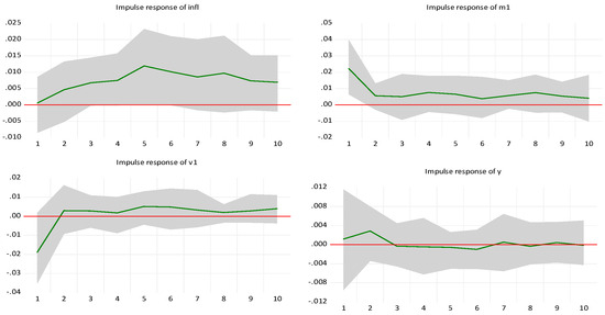
Figure 1.
ITA IRFs with a shock in m1 (Uhlig rejection method).
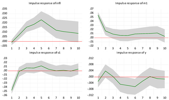
Figure 2.
ITA IRFs with a shock in m1 (Uhlig penalty method).
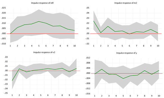
Figure 3.
ITA IRFs with a shock in m2 (Uhlig rejection method).
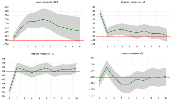
Figure 4.
ITA IRFs with a shock in m2 (Uhlig penalty method).
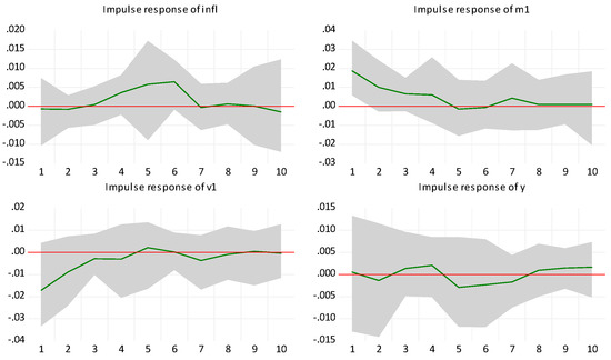
Figure 5.
JPN IRFs with a shock in m1 (Uhlig rejection method).
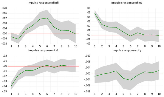
Figure 6.
JPN IRFs with a shock in m1 (Uhlig penalty method).
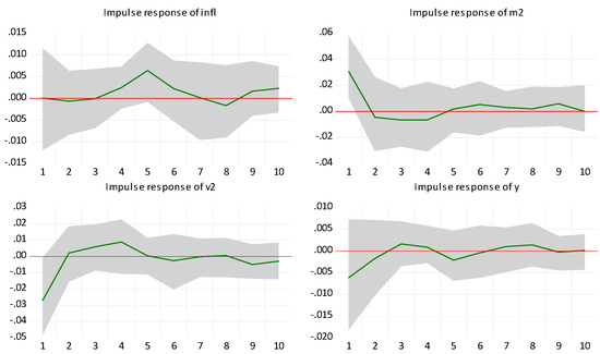
Figure 7.
JPN IRFs with a shock in m2 (Uhlig rejection method).
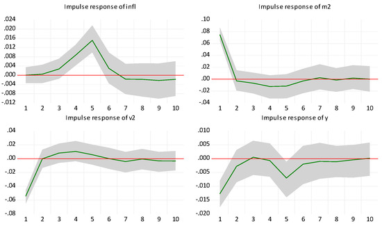
Figure 8.
JPN IRFs with a shock in m2 (Uhlig penalty method).
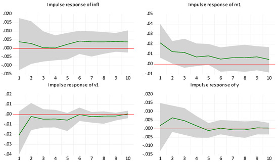
Figure 9.
UK IRFs with a shock in m1 (Uhlig rejection method).
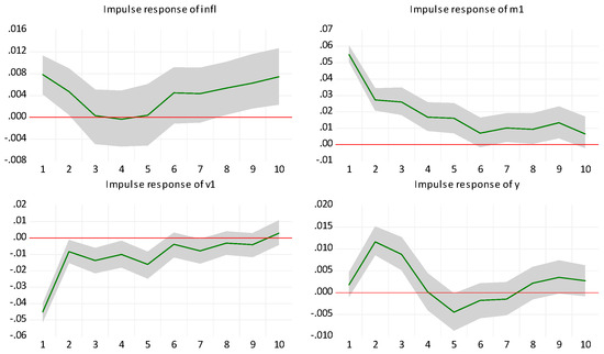
Figure 10.
UK IRFs with a shock in m1 (Uhlig penalty method).
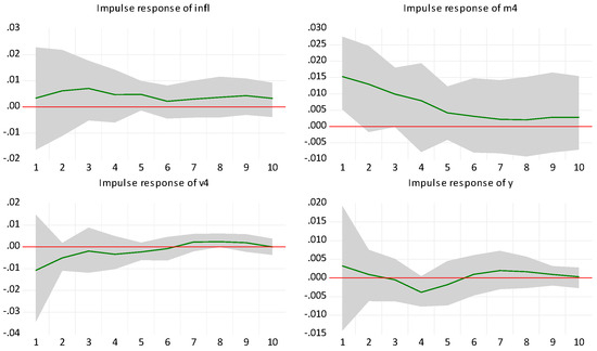
Figure 11.
UK IRFs with a shock in m4 (Uhlig rejection method).
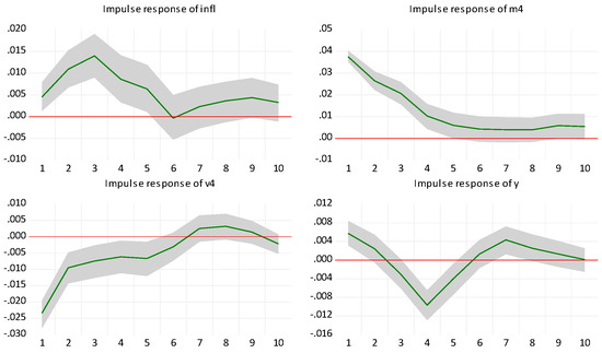
Figure 12.
UK IRFs with a shock in m4 (Uhlig penalty method).
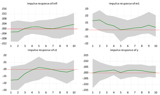
Figure 13.
USA IRFs with a shock in m1 (Uhlig rejection method).
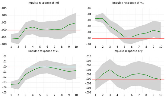
Figure 14.
USA IRFs with a shock in m1 (Uhlig penalty method).
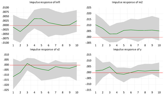
Figure 15.
USA IRFs with a shock in m2 (Uhlig rejection method).
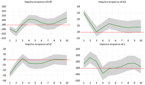
Figure 16.
USA IRFs with a shock in m2 (Uhlig penalty method).
These diagrams show that the impact of a shock in m on inflation dynamics varies across different situations. More in detail, disentangling the variables reveals that m has the largest effect (m1, m2, and m4 for UK) when compared with y and v. This phenomenon is especially noticeable during the initial period and applies to all graphs. In the medium term, the trajectory appears to be declining. Both monetary aggregates exhibit significant long-term persistence in the USA and the UK cases. Another important feature to observe is the dynamics of the variables themselves. The movements of variables v and y do not appear to support the Monetarist approach and its assumption of their irrelevance within the mechanism (by assigning a value of zero to both). The findings show that the monetary shock reduces v (at least) in the first phase of the shock. This is plausible because the system, especially the private sector, does not immediately absorb any “injection of new money”. For instance, the new credit is not immediately allocated or used for consumption or investment. Therefore, the resulting transmission mechanism will be slower. Nevertheless, even if with different features, it is reasonable to posit that a similar phenomenon could occur in the public sector. There is no confirmation of the “neutrality of money axiom” regarding the relationship between y and m. The graphs illustrate a counteracting effect of GDP growth y on monetary dynamics m. Indeed, the positive shock in m is followed by a corresponding shock in y. However, since y has a negative algebraic sign in (3), it can be observed that it exhibits consistent behavior within the TQM framework.
Figure 17, Figure 18, Figure 19, Figure 20, Figure 21, Figure 22, Figure 23 and Figure 24 display the IRF of the SVAR analysis conducted on the second dataset.
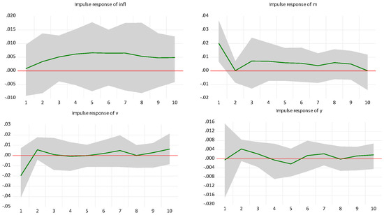
Figure 17.
ITA IRFs with a shock in broad money (Uhlig rejection method).
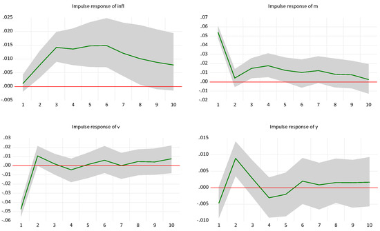
Figure 18.
ITA IRFs with a shock in broad money (Uhlig penalty method).
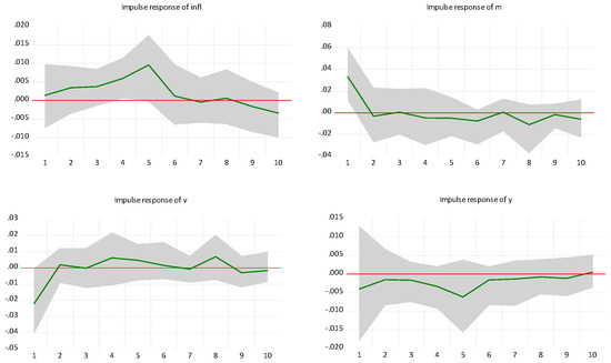
Figure 19.
JPN IRFs with a shock in broad money (Uhlig rejection method).
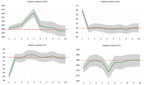
Figure 20.
JPN IRFs with a shock in broad money (Uhlig penalty method).
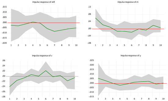
Figure 21.
UK IRFs with a shock in broad money (Uhlig rejection method).
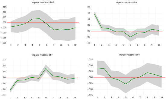
Figure 22.
UK IRFs with a shock in broad money (Uhlig penalty method).
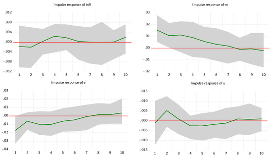
Figure 23.
USA IRFs with a shock in broad money (Uhlig rejection method).
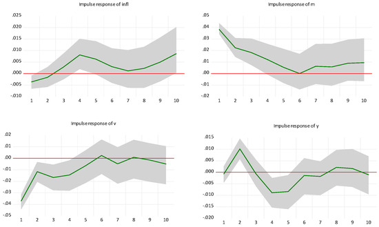
Figure 24.
USA IRFs with a shock in broad money (Uhlig penalty method).
The second set of results also confirms the prominent role of the monetary variable m in the model. As in the first dataset, the greatest impact occurs in the very early period and then diminishes over time. Nevertheless, in only one case (the USA) does m demonstrate a certain degree of persistence. In fact, in three out of four cases, the effect is evident in period 1, while it fades afterwards. The fairly similar time span for the case of Japan in the two subsets confirms the results (the differences are certainly due to the different specification of the monetary aggregates in the second dataset). v and y have an effect; they are not zero. In addition, the sign of y has an opposite effect on m and π. The response of v to the initial monetary shock is negative. This dynamic is also a confirmation of the results of the first data set.
Overall, our SVAR results confirm that m has a (positive) impact on π but, at the same time, there is evidence of an opposite effect exerted by y, and that the highest impact of m on π is triggered in the very early phase of the shock. In the long run, the effect of m is not so persistent. Basically, this situation applies to both subsets. With respect to the three countries (ITA, JPN, and USA), for which the series are almost identical in length (but differ in the inclusion of the pre- and post-pandemic periods), there are no particular differences with the updated series, which also include the very first measures prepared to deal with crisis-related imbalances (in support of the ergodic axiom). The strong empirical correlation between money growth and inflation is documented by De Grauwe and Polan (2005), Teles et al. (2016), and Agur et al. (2022), but in a context characterized by the presence of an averagely high level of inflation. These latter results are consistent with the mathematical relationship shown in Section 2, where we emphasized that m = π condition holds only for not very high values of π. Moreover, Agur et al. (2022) found no evidence of a systematic effect of MF announcements on inflation expectations when the CBs took explicit measures to purchase bonds in the primary market during the COVID-19 pandemic. In the terms of the present research objective, these results are not compatible with a strictly Monetarist view, which posits that an increase in the monetary base results in structural inflation. Our results are consistent with the strand of literature that does not address the mechanism following this radical interpretation of QTM. Even if m is shown to be the most influential variable, the effects of v and y are not equal to 0. The variables m, v, and y have a combined impact on the inflation path as suggested by the original QTM model. This has significant implications for economic policy as it demonstrates the potential for MF to serve as a pivotal instrument for facilitating economic recovery. Agur et al. (2022) accurately note that the relationship between money growth and inflation heavily depends on economic conditions and institutional factors.
5. Conclusions
The pandemic and the Russia–Ukraine crisis have induced new economic and social costs. The same thing is repeated with every major economic shock. Will the Israel–Hamas crisis raise the same concerns again? In this scenario, the ability of certain governments to finance public spending is severely limited. To support expenditures related to exceptional circumstances, (so-called) conventional instruments have clear limitations. This is the main problem. The purpose of this paper is to examine the reintroduction of MF as a tool to support growth-oriented economic policies. The analysis is centered on the well-known QTM which, in the most prevalent interpretation, is arguably misconstrued. Our results support these concerns. On the operational level, understanding the importance of liquidity in determining the flow of production and employment is crucial for an entrepreneurial system (Davidson 2015). Although there is a common trend, the existing asymmetries across countries’ economic systems will exacerbate. In terms of economic policy options, both fiscal and monetary actions have their relative merits and drawbacks. For many countries, the fiscal position is expected to worsen, leading to an increase in total public debt. In such cases, it is particularly important to monitor the corresponding government’s debt to GDP ratio. Given these concerns, it is difficult to attribute the current inflation dynamic to excessive demand. Supply reductions and bottlenecks due to the resulting pressures on global supply chains are the next problems to be addressed. Supply-side recessions can lead to concerns about a resurgence of inflation. The recent literature has investigated the neutralizing impact of monetary policies in supply-side crises (Bhattacharya and Jain 2020; Ginn and Pourroy 2020; Iddrisu and Alagidede 2020). Celasun et al. (2022) and di Giovanni et al. (2022) published papers that discuss the impact of supply constraints on economies and inflation. Shapiro (2022) points out the impact of supply-driven factors during recessions with monetary tightening. Such positions are consistent with the analysis of the price inflation proposed by Weintraub (1961) according to which decreasing productivity inversely affects prices in the supply price of industrial goods equation (Kaldor 1975). Explained in a different way, some authors favor the idea that—for the USA—post-COVID-19 inflation is the result of shocks to prices given wages (Bernanke and Blanchard 2023). Some inflation may be necessary to manage high debts (Randall Wray 2015). The interconnection of global economic systems and their relationship with real prices and financial markets, such as commodities, is an additional factor to consider. Uncertainty-related fluctuations that could occur in financial markets due to conflicts are reported, with particular reference to the equity segment, for example, in Brune et al. (2015). If we view the situation through the lens of the QTM, it is necessary to stimulate the economic system by implementing measures that promote output growth. This can assist with managing debt. Although the QTM is old, the debate on how to handle sudden macroeconomic shocks is bringing renewed attention to it. This is at the core of MF and its implementation. Opponents of MF advocate against it mainly due to the fear of inflation or hyperinflation linked to an excessive money supply. The connection between inflation and monetary aggregates is central to the QTM, so rediscovering and analyzing it empirically does not appear to be a futile exercise.
There are four levers that policymakers can use to maintain the sustainability of debt and its service: tight fiscal policy (austerity), debt defaults or restructurings, MF, and redistributing money and credit from those who have more to those who have less (Dalio 2018).
In certain countries, austerity measures have been in place for an extended period of time. Insolvency and/or debt restructuring could harm the credibility of governments. Finally, the fourth option would be challenging to explain to those who have acquired wealth without committing tax fraud. Even if we assume the presence of nominal rigidities in prices, as documented by Gopinat and Itskhoki (2010), Klenow and Kryvtsov (2008) and Nakamura and Steinsson (2008), the MF can lead to a modest but permanent expansionary period that QE could not (and cannot) guarantee (Agur et al. 2022). Our findings show that monetary shock fuels inflation in the early stages. The importance of MF as a tool for dealing with macroeconomic imbalances that have already been created (or may occur in the future) as a result of significant shocks is underscored by the results of this work. The current causes of inflation do not appear to be due to excess demand, but rather seem to be related to supply shocks. These elements have the potential to inform policy implications. In fact, the adoption of MF could be beneficial in maintaining the liquidity required by the entire economic system, while also promoting economic growth to support the debt. In a market-oriented, money-using entrepreneurial economy, the restriction of production activities is a risk of contraction in supply with a subsequent high possibility of stagflation. The optimal deployment of MF has the potential to serve as an efficacious instrument for confronting the economic challenges that can culminate in unsustainable debt.
Based on these considerations, future research developments may potentially encompass an expansion of the number of countries included. For example, it will be interesting investigate countries not included in the classical “western World”. The sole limiting factor will be the availability of data for processing.
Author Contributions
Conceptualization: A.F. (Antonio Focacci) and A.F. (Angelo Focacci); Methodology, Validation, Formal Analysis, Investigation, Resources, Data Curation, Writing-original draft preparation, review and editing, visualization, supervision, project administration: A.F. (Antonio Focacci). Software: EVIEWS version 11 and version 13. All authors have read and agreed to the published version of the manuscript.
Funding
This research received no external funding.
Data Availability Statement
All data used in the study are available from the corresponding author upon request.
Acknowledgments
The authors wish to thank the Editor-in-Chief, one anonymous Academic Editor and five anonymous reviewers for their stimulating activity in improving the very first version of the manuscript.
Conflicts of Interest
The authors declare no conflicts of interest.
References
- Abid, Amira, and Fathi Abid. 2024. Sovereign credit risk in Saudi Arabia, Morocco and Egypt. Journal of Risk and Financial Management 17: 283. [Google Scholar] [CrossRef]
- Acocella, Nicola. 2014. Fondamenti di Politica Economica, 5th ed. Rome: Carocci Editore. [Google Scholar]
- Afonso, Anotonio, José Alves, and Raquel Balhote. 2019. Interactions between monetary and fiscal policies. Journal of Applied Economics 22: 132–51. [Google Scholar] [CrossRef]
- Agur, Itai, Darmien Capelle, Giovanni Dell’Ariccia, and Damiano Sandri. 2022. Monetary Finance. Do Not Touch, or Handle with Care? Departmental Paper DP/2022/001. Washington, DC: International Monetary Fund. [Google Scholar]
- Arcand, Jean-Louis, Enrico Berkes, and Ugo Panizza. 2015. Too much finance? Journal of Economic Growth 20: 105–48. [Google Scholar] [CrossRef]
- Arias, Jonas E., Juan F. Rubio-Ramìrez, and Daniel F. Waggoner. 2018. Inference based on structural vector autoregressions identified with sign and zero restrictions: Theory and applications. Econometrica 86: 685–720. [Google Scholar] [CrossRef]
- Aroul, Ramya R., Noura K. Kone, and Sanjiv Sabherval. 2024. Financial distress premium or discount? Some new evidence. Journal of Risk Financial Management 17: 286. [Google Scholar] [CrossRef]
- Assenmacher-Wesche, Katrin, and Stefan Gerlach. 2008. Interpreting Euro area inflation at high and low frequencies. European Economic Review 52: 964–86. [Google Scholar] [CrossRef]
- Banca d’Italia. 2023. Banca d’Italia Web Data Bank. Available online: https://infostat.bancaditalia.it/inquiry/home?spyglass/taxo:CUBESET=/PUBBL_00/PUBBL_00_02_01_04/PUBBL_00_02_01_04_03&ITEMSELEZ=AGGM0100:true&OPEN=true/&ep:LC=IT&COMM=BANKITALIA&ENV=LIVE&CTX=DIFF&IDX=2&/view:CUBEIDS=AGGM0100 (accessed on 21 September 2023).
- Bank of England. 2023a. Consumer Price Inflation in the United Kingdom [CPIIUKA], Retrieved from FRED, Federal Reserve Bank of St. Louis. Available online: https://fred.stlouisfed.org/series/CPIIUKA (accessed on 5 May 2023).
- Bank of England. 2023b. M1 Money Stock in the United Kingdom [MSM1UKQ], Retrieved from FRED, Federal Reserve Bank of St. Louis. Available online: https://fred.stlouisfed.org/series/MSM1UKQ (accessed on 5 May 2023).
- Barbiellini Amidei, Federico, Riccardo De Bonis, Miria Rocchelli, Alessandra Salvio, and Massimiliano Stacchini. 2016. La Moneta in Italia dal 1861: Evidenze da un Nuovo Dataset. Questioni di Economia e Finanza (Occasional Papers), Issue 328. Rome: Banca d’Italia, April. [Google Scholar]
- Basco, Emiliano, Laura D’Amato, and Maria Garegnani. 2009. Understanding the money-prices relationship under low and high inflation regimes: Argentina 1977–2006. Journal of International Money and Finance 28: 1182–203. [Google Scholar] [CrossRef]
- Baumeister, Christiane, and James D. Hamilton. 2015. Sign restrictions, structural vector autoregressions, and useful prior information. Econometrica 83: 1963–99. [Google Scholar] [CrossRef]
- Belke, Ansgar, Ingo G. Bordon, and Ulrich Volz. 2012. Effects of global liquidity on commodity and food prices. World Development 44: 31–43. [Google Scholar] [CrossRef]
- Benati, Luca. 2009. Long-Run Evidence on Money-Growth and Inflation. Working Paper no. 1027. Frankfurt: European Central Bank. Available online: https://www.ecb.europa.eu/pub/pdf/scpwps/ecbwp1027.pdf (accessed on 16 March 2020).
- Bernanke, Ben. 1986. Alternative explanations of the money-income correlation. Carnegie-Rochester Conference Series on Public Policy 25: 49–99. [Google Scholar] [CrossRef]
- Bernanke, Ben, and Olivier Blanchard. 2023. What Caused the US Pandemic-Era Inflation? Working Paper #86. Hutchins: Hutchins Center on Fiscal & Monetary Policy, June, Available online: https://www.brookings.edu/research/what-caused-the-u-s-pandemic-era-inflation/ (accessed on 15 December 2023).
- Berndt, Antje, and Șevin Yeltekin. 2015. Monetary policy, bond returns and debt dynamics. Journal of Monetary Economics 73: 119–36. [Google Scholar] [CrossRef]
- Bhattacharya, Rudrani, and Richa Jain. 2020. Can monetary policy stabilize food inflation? Evidence from advanced and emerging economies. Economic Modelling 89: 122–41. [Google Scholar] [CrossRef]
- Blanchard, Olivier J. 1990. Why does money affect output? In Handbook of Monetary Economics. Edited by Benjamin Friedman and Franck Hahn. New York: North Holland, vol. 2, p. 828. [Google Scholar]
- Blanchard, Olivier J., and Danny Quah. 1989. The dynamic effects of aggregate demand and supply disturbances. American Economic Review 79: 655–73. [Google Scholar]
- Blanchard, Olivier J., and Jean Pisani-Ferry. 2020. Monetisation: Do Not Panic. VoxEU. Org. April 10. Available online: https://voxeu.org/article/monetisation-do-not-panic (accessed on 25 April 2023).
- Blanchard, Olivier J., Giovanni Dell’Ariccia, and Paolo Mauro. 2010. Rethinking macroeconomic policy. Journal of Money, Credit and Banking 42: 199–215. [Google Scholar] [CrossRef]
- Blinder, Alan, and Robert Solow. 1973. Does fiscal policy matter? Journal of Public Economics 2: 319–37. [Google Scholar] [CrossRef]
- Board of Governors of the Federal Reserve System (US). 2023. M2 Money Stock [M2NS], Retrieved from FRED, Federal Reserve Bank of St. Louis. Available online: https://fred.stlouisfed.org/series/M2NS (accessed on 5 May 2023).
- Bolt, Jutta, Robert Inklaar, Herman de Jong, and Jan Luiten van Zanden. 2018. Rebasing “Maddison”: New Income Comparisons and the Shape of Long-Run Economic Development. Maddison Project Working Paper 10. Available online: https://www.rug.nl/ggdc/historicaldevelopment/maddison/releases/maddison-project-database-2018?lang=en (accessed on 20 February 2020).
- Brune, Amelie, Thorsten Hens, Marc Rieger, and Mei Wang. 2015. The war puzzle: Contradictory effects of international conflicts on stock markets. International Review of Economics 62: 1–21. [Google Scholar] [CrossRef]
- Buiter, Willem. 2014. The simple analytics of helicopter money. Why it works-always. Economics–The Open Access. Open Assessment E-Journal 8: 2014–28. [Google Scholar] [CrossRef]
- Buiter, Willem. 2020. Central Banks as Fiscal Players: The Drivers of Fiscal and Monetary Policy Space. Federico Caffè Lectures. Cambridge: Cambridge University Press. [Google Scholar]
- Canova, Fabio. 2007. Methods for Applied Macroeconomic Research. Princeton: Princeton University Press. [Google Scholar]
- Canova, Fabio, and Gianni De Nicolò. 2002. Monetary disturbances matter for business fluctuations in the G-7. Journal of Monetary Economics 49: 1131–59. [Google Scholar] [CrossRef]
- Celasun, Oya, Niels-Jacob Hansen, Aiko Mineshima, Mariano Spector, and Jing Zhou. 2022. Supply Bottlenecks: Where, Why, How Much, and What Next? Working Paper 22/31 February. Washington, DC: International Monetary Fund. Available online: https://www.imf.org/en/Publications/WP/Issues/2022/02/15/Supply-Bottlenecks-Where-Why-How-Much-and-What-Next-513188 (accessed on 9 March 2023).
- Chang, Chih-Hsang, Kam C. Chan, and Hung-Gay Fung. 2009. Effect of money supply on real output and price in China. China and World Economy 17: 35–44. [Google Scholar] [CrossRef]
- Christensen, Michael. 2001. Real supply shocks and the money–growth–inflation relationship. Economics Letters 72: 67–72. [Google Scholar] [CrossRef]
- Crowder, William J. 1998. The long-run link between money growth and inflation. Economic Inquiry 36: 229–43. [Google Scholar] [CrossRef]
- Cukierman, Alex. 2017. Money growth and inflation:policy lessons from a comparison of the US since 2008 with hyperinflation Germany in the 1920s. Economics Letters 154: 109–12. [Google Scholar] [CrossRef]
- Dalio, Ray. 2018. Principles for Navigating Big Debt Crises. Part I: The Archetypal Big Debt Cycle. Westport: Bridgewater. [Google Scholar]
- Davidson, Paul. 2015. Post-Keynesian Theory and Policy. A Realistic Analysis of the Market Oriented Capitalist Economy. Northampton: Edward Elgar. [Google Scholar]
- De Grauwe, Paul. 2020. The need for monetary financing of corona budget deficits. Intereconomics 55: 133–34. [Google Scholar] [CrossRef]
- De Grauwe, Paul, and Magdalena Polan. 2005. Is inflation always and everywhere a monetary phenomenon? The Scandinavian Journal of Economics 107: 239–59. [Google Scholar] [CrossRef]
- Dell’Ariccia, Giovanni, Pau Rabanal, and Damiano Sandri. 2018. Unconventional monetary polizie in the Euro area, Japan and the United Kingdom. Journal of Economic Perspectives 32: 147–72. [Google Scholar] [CrossRef]
- di Giovanni, Julian, Şebnem Kalemli-Özcan, Alvaro Silva, and Muhammed Yildirim. 2022. Global Supply Chain Pressures, International Trade, and Inflativo. NBER Working Paper No. 30240. Available online: https://www.nber.org/papers/w30240 (accessed on 16 August 2023).
- Doan Van, Dinh. 2020. Money supply and inflation impact on economic growth. Journal of Financial Economic Policy 12: 121–36. [Google Scholar] [CrossRef]
- Ellington, Michael, and Costas Milas. 2019. Global liquidity, money growth and UK inflation. Journal of Financial Stability 42: 67–74. [Google Scholar] [CrossRef]
- Escanciano, Juan Carlos, Ignacio Lobato, and Lin Zhu. 2013. Automatic diagnostic checking for vector autoregressions. Journal of Business and Economic Statistics 31: 426–37. [Google Scholar] [CrossRef]
- Falck, Elisabeth, Mathias Hoffmann, and Patrick Hürtgen. 2021. Disagreement about inflation expectations and monetary policy transmission. Journal of Monetary Economics 118: 15–31. [Google Scholar]
- Faust, Jon. 1998. The Robustness of Identified VAR Conclusions about Money. Carnegie-Rochester Conference Series on Public Policy 49: 207–44. [Google Scholar]
- Fed. 2023a. Federal Reserve Bank of Saint Louis. Velocity of M1 Money Stock. Available online: https://fred.stlouisfed.org/series/M1V (accessed on 30 September 2023).
- Fed. 2023b. Federal Reserve Bank of Saint Louis. Velocity of M2 Money Stock. Available online: https://fred.stlouisfed.org/series/M2V (accessed on 30 September 2023).
- Fisher, Irving. 1911. The Purchasing Power of Money: Its Determination and Relation to Credit, Interest and Crises. New York: The Macmillan Company. [Google Scholar]
- Focacci, Aantonio. 2023a. Is this very much a matter of faith? A monetization approach to COVID-19. International Journal of Business and Systems Research 17: 347–66. [Google Scholar] [CrossRef]
- Focacci, Antonio. 2023b. Money-growth and inflation: A wavelet analysis for a monetization approach to COVID-19. Challenge 66: 27–48. [Google Scholar] [CrossRef]
- Focacci, Antonio, Angelo Focacci, and Alessandro Faenza. 2024. The lens of the quantity theory of money to disentangle the perceived relationship between mony growth and inflation: A PSVAR approach. Eurasian Economic Review. Available online: https://link.springer.com/article/10.1007/s40822-024-00269-9 (accessed on 4 July 2024).
- Friedman, Milton. 1956. The quantity theory of money: A restatement. In Studies in the Quantity Theory of Money. Edited by Milton Friedman. Chicago: University of Chicago Press, pp. 3–21. [Google Scholar]
- Friedman, Milton. 1963a. Inflation: Causes and Consequences. Bombay: Asian Publishing House. [Google Scholar]
- Friedman, Milton. 1963b. Monetarism in Rhetoric and in Practice. Bank of Japan Monetary and Economic Studies 2: 1–14. [Google Scholar]
- Friedman, Milton. 1970. A theoretical framework for monetary analysis. Journal of Political Economy 78: 193–238. [Google Scholar] [CrossRef]
- Friedman, Milton. 1992. Money Mischief: Episodes in Monetary History. New York: Harcourt Brace Jovanovich. [Google Scholar]
- Fry, Renée, and Adrian Pagan. 2011. Sign restrictions in structural vector autoregressions: A critical view. Journal of Economic Literature 49: 938–60. [Google Scholar] [CrossRef]
- Galì, Jordi. 1992. How well does the ISLM model fit postwar US data. The Quarterly Journal of Economics 107: 709–38. [Google Scholar] [CrossRef]
- Galì, Jordi. 2020a. Helicopter Money: The Time Is Now. CEPR, VoxEU. Org. March 17. Available online: https://cepr.org/voxeu/columns/helicopter-money-time-now (accessed on 7 May 2023).
- Galì, Jordi. 2020b. The effects of a money-financed fiscal stimulus. Journal of Monetary Economics 115: 1–19. [Google Scholar] [CrossRef]
- Giavazzi, Francesco, and Guido Tabellini. 2020. Covid Perpetual Bonds: Jointly Guaranteed and Supported by the ECB. CEPR, VoxEU. Org. March 24. Available online: https://voxeu.org/article/covid-perpetual-eurobonds (accessed on 7 May 2023).
- Ginn, William, and Marc Pourroy. 2020. Should a central bank react to food inflation? Evidence from an estimated model for Chile. Economic Modelling 90: 221–34. [Google Scholar] [CrossRef]
- Gopinat, Gita, and Oleg Itskhoki. 2010. Frequency of price adjustment and pass through. The Quarterly Journal of Economics 125: 675–727. [Google Scholar] [CrossRef]
- Graff, Michael. 2008. The Quantity Theory of Money in Historical Perspective. KOF Working Papers 196. Available online: https://www.research-collection.ethz.ch/handle/20.500.11850/124095 (accessed on 20 January 2024).
- Guncor, Cahit, and Ali Berk. 2006. Money supply and inflation relationship in the Turkish economy. Journal of Applied Sciences 6: 2083–87. [Google Scholar] [CrossRef][Green Version]
- Hall, Stephen, George Hondroyiannis, Paravastu A. V. B. Swamy, and George Tavlas. 2009. Assessing the causal relationship between Euro-area money and prices in a time-varying environment. Economic Modelling 26: 760–66. [Google Scholar] [CrossRef]
- Hamilton, James D., and Ana Maria Herrera. 2004. Oil shocks and aggregate macroeconomic behavior: The role of monetary policy. Journal of Money, Credit, and Banking 36: 265–86. [Google Scholar] [CrossRef]
- Haug, Alfred, and William Dewald. 2004. Longer-Term Effects of Monetary Growth on Real and Nominal Variables, Major Industrial Countries: 1880–2001. Working Paper No. 382. Frankfurt: European Central Bank. Available online: https://www.ecb.europa.eu/pub/pdf/scpwps/ecbwp382.pdf (accessed on 12 June 2021).
- Hudson, Michael. 2021. Finance capitalism versus industrial capitalism: The Rentier resurgence and takeover. Review of Radical Political Economics 53: 557–73. [Google Scholar] [CrossRef]
- Iddrisu, Abdul-Aziz, and Imhotep P. Alagidede. 2020. Monetary policy and food inflation in South Africa: A quantile regression analysis. Food Policy 91: 101816. [Google Scholar] [CrossRef]
- IMF. 2009. From recession to recovery: How strong and how soon? In IMF World Economic Outlook. Washington, DC: International Monetary Fund. Available online: https://www.elibrary.imf.org/display/book/9781589068063/ch003.xml (accessed on 6 May 2022).
- IMF. 2020a. International Financial Statistics. Available online: https://data.imf.org/?sk=4c514d48-b6ba-49ed-8ab9-52b0c1a0179b (accessed on 8 October 2020).
- IMF. 2020b. M1 for United States [MYAGM1USM052S], Retrieved from FRED, Federal Reserve Bank of St. Louis. Available online: https://fred.stlouisfed.org/series/MYAGM1USM052S (accessed on 8 October 2020).
- IMF. 2020c. M4 for United Kingdom [MYAGM4GBM189S], Retrieved from FRED, Federal Reserve Bank of St. Louis. Available online: https://fred.stlouisfed.org/series/MYAGM4GBM189S (accessed on 8 October 2020).
- IMF. 2021. World Economic Outlook Database: April. Available online: https://www.imf.org/en/Publications/WEO/weo-database/2021/April/weo-report?a=1&c=001,&s=NGDP_RPCH,&sy=2019&ey=2020&ssm=0&scsm=1&scc=0&ssd=1&ssc=0&sic=0&sort=country&ds=.&br=1 (accessed on 27 June 2021).
- It.inflation. 2020. Inflation.eu Website. Available online: https://www.inflation.eu/it/ (accessed on 5 May 2020).
- Ivanov, Ventizlav, and Lutz Kilian. 2005. A practitioner’s guide to lag order selection for VAR impulse response analysis. Studies in Nonlinear Dynamics & Econometrics 9: 2. Available online: http://drphilipshaw.com/Protected/A%20Practitioners%20Guide%20to%20Lag%20Order%20Selection%20for%20VAR%20Impulse%20Response%20Analysis.pdf (accessed on 22 July 2023).
- Kaldor, Nicholas. 1975. What is wrong with economic theory. The Quarterly Journal of Economics 89: 347–57. [Google Scholar] [CrossRef]
- Kapoor, Sony, and Willem Buiter. 2020. To Fight the Covid Pandemic, Policymakers Must Move Fast and Break Taboos. CEPR, VoxEU. Org. April 6. Available online: https://cepr.org/voxeu/columns/fight-covid-pandemic-policymakers-must-move-fast-and-break-taboos (accessed on 7 May 2023).
- Kawai, Masahiro, and Peter Morgan. 2013. Banking Crises and “Japanization”: Origins and Implications. Asian Development Bank Institute Working Paper 430. Tokyo: Asian Development Bank Institute. Available online: https://www.adb.org/publications/banking-crises-and-japanization-origins-and-implications (accessed on 20 April 2023).
- Kilian, Lutz. 2001. Impulse response analysis in vector autoregressions with unknown lag order. Journal of Forecasting 20: 161–79. [Google Scholar] [CrossRef]
- Kilian, Lutz, and Daniel Murphy. 2012. Why agnostic sign restrictions are not enough: Understanding the dynamics of oil market VAR models. Journal of the European Economic Association 10: 1166–88. [Google Scholar] [CrossRef]
- Klenow, Peter, and Oleksiy Kryvtsov. 2008. State-dependent or time-dependent pricing: Does it matter for recent US inflation? The Quarterly Journal of Economics 123: 863–904. [Google Scholar] [CrossRef]
- Kuttner, Kenneth. 2018. Outside the box: Unconventional monetary policy in the Great Recession and beyond. Journal of Economic Perspectives 32: 121–46. [Google Scholar] [CrossRef]
- Lucas, Deborah, and Refet Gürkaynak. 2020. Funding Pandemic Relief: Monetise Now. CEPR, VoxEU. Org. May 14. Available online: https://cepr.org/voxeu/columns/funding-pandemic-relief-monetise-now (accessed on 7 May 2023).
- Lütkepohl, Helmut. 2005. New Introduction to Multiple Series Analysis. Berlin: Springer. [Google Scholar]
- Makin, Anthony J., Alex Robson, and Shyama Ratnasiri. 2017. Missing money found causing Australia’s inflation. Economic Modelling 66: 156–62. [Google Scholar] [CrossRef]
- Mardanov, Ismatilla. 2023. Issues of EU member nation’s shared sovereignty, institutions, and economic development. Economies 11: 128. [Google Scholar] [CrossRef]
- McCandless, George, and Weber Warren. 1995. Some monetary facts. Federal Reserve Bank of Minneapolis Quarterly Review 19: 2–11. [Google Scholar] [CrossRef]
- Müller, Ulrick, and Mark Watson. 2018. Long-run covariability. Econometrica 86: 775–804. [Google Scholar] [CrossRef]
- Nakamura, Emi, and Jón Steinsson. 2008. Five facts about prices: A reevaluationof menu cost models. The Quarterly Journal of Economics 123: 1415–64. [Google Scholar] [CrossRef]
- Nicoletti Altimari, Sergio. 2001. Does Money Lead Inflation in the Euro Area? Working Paper No. 63. Frankfurt: European Central Bank. Available online: https://www.ecb.europa.eu/pub/pdf/scpwps/ecbwp063.pdf (accessed on 23 June 2019).
- OCPI. 2023. Osservatorio dei Conti Pubblici Italiani. Available online: https://osservatoriocpi.unicatt.it/ocpi-servizi-serie-storiche (accessed on 27 June 2023).
- OECD. 2020. M1 for Japan [MANMM101JPA657S], Retrieved from FRED, Federal Reserve Bank of St. Louis. Available online: https://fred.stlouisfed.org/series/MANMM101JPA657S (accessed on 8 October 2020).
- Palley, Thomas. 1998. The twin circuits: Aggregate demand and the expenditure multiplier in a monetary economy. Review of Radical Political Economics 30: 91–101. [Google Scholar] [CrossRef]
- Palley, Thomas. 2020. What’s wrong with Modern Money Theory: Macro and political economic restraints on deficit-financed fiscal policy. Review of Keynesian Economics 8: 472–93. [Google Scholar] [CrossRef]
- Panizza, Ugo, and Andrea Presbitero. 2014. Public debt and economic growth: Is there a causal effect? Journal of Macroeconomics 41: 21–41. [Google Scholar] [CrossRef]
- Petrakos, George, Konstantinos Rontos, Chara Vavoura, and Ioannis Vavouras. 2023. The impact of recent economic crises on income inequality and the risk of poverty in Greece. Economies 11: 166. [Google Scholar] [CrossRef]
- Pisani-Ferry, Jean, and Olivier J. Blanchard. 2020. Monetisation: Do Not Panic. CEPR, VoxEU. Org. April 10. Available online: https://cepr.org/voxeu/columns/monetisation-do-not-panic (accessed on 7 May 2023).
- Plikas, John H., Dimitrios Kenourgios, and Georgios A. Savvakis. 2024. COVID-19 and Non-performing loans in Europe. Journal of Risk and Financial Management 17: 271. [Google Scholar] [CrossRef]
- Randall Wray, Larry. 2015. Modern Money Theory. A Primer on Macroeconomics for Sovereign Monetary Systems, 2nd ed. Basingstoke: Palgrave Macmillan. [Google Scholar]
- Sargent, Thomas J., and Neil Wallace. 1981. Some unpleasant monetarist arithmetic. Federal Reserve Bank of Minneapolis Quarterly Review 5: 1–17. [Google Scholar] [CrossRef]
- Schwarz, Thomas, and Andrew Szakmary. 1994. Price discovery in petroleum markets: Arbitrage, cointegration, and the time interval of analysis. Journal of Futures Markets 14: 147–67. [Google Scholar] [CrossRef]
- Serkov, Leonid, Sergey Krasnykh, Julia Dobrovskaya, and Elena Kozonogova. 2024. The feasibility of coordinating international monetary policy strategies in the context of asymmetric demand shocks. Journal of Risk and Financial Management 17: 259. [Google Scholar] [CrossRef]
- Shapiro, Adam. 2022. Decomposing Supply and Demand Driven Inflation; San Francisco: Federal Reserve Bank of San Francisco. Available online: https://www.frbsf.org/research-and-insights/publications/working-papers/2022/10/decomposing-supply-and-demand-driven-inflation/ (accessed on 5 July 2024).
- Sims, Christopher. 1980. Macroeconomics and reality. Econometrica 48: 1–48. [Google Scholar] [CrossRef]
- Sims, Christopher, James Stock, and Mark Watson. 1990. Inference in linear time series models with some unit roots. Econometrica 58: 113–44. [Google Scholar] [CrossRef]
- Teles, Pedro, Harald Uhlig, and João Valle e Azevedo. 2016. Is quantity theory of money still alive? The Economic Journal 126: 442–64. [Google Scholar] [CrossRef]
- Thomas, Ryland, and Samuel Williamson. 2023. What Was the UK GDP Then? The Historic Series, Measuringworth. Available online: https://www.measuringworth.com/datasets/ukgdp/ (accessed on 27 June 2023).
- Turner, Adair. 2015. The case for monetary finance-an essentially political issue. Presented at the 16th Jacques Polak Annual Research Conference Hosted by the International Monetary Fund, Washington, DC, USA, November 5–6; Available online: https://www.imf.org/external/np/res/seminars/2015/arc/pdf/adair.pdf (accessed on 20 June 2023).
- Uhlig, Harald. 2005. What are the effects of monetary policy on output? Results from an agnostic identification procedure. Journal of Monetary Economics 52: 381–419. [Google Scholar] [CrossRef]
- Uhlig, Harald. 2017. Shocks, sign restrictions, and identification. In Advances in Economics and Econometrics 11th World Congress-Econometric Society Monograph. Edited by Bo Honoré, Ariel Pakes, Monika Piazzesi and Larry Samuelson. Cambridge: Cambridge University Press, pp. 95–127. [Google Scholar]
- Weintraub, Sidney. 1961. Classical Keynesianism Monetary Theory and the Price Level. Philadelphia and New York: Chilton Company. [Google Scholar]
- Williamson, Samuel. 2023. What Was the US GDP Then? Measuringworth. Available online: https://www.measuringworth.com/datasets/usgdp/ (accessed on 27 June 2023).
- Wold, Herman. 1951. Dynamic systems of the recursive type-Economic and statistical aspects. Sankhyā 11: 205–17. [Google Scholar]
- World Bank. 2020. Inflation, Consumer Prices for the United States, Retrieved from FRED, Federal Reserve Bank of St. Louis. Available online: https://fred.stlouisfed.org/series/FPCPITOTLZGUSA (accessed on 8 October 2020).
- World Bank. 2021. World Development Indicators. Available online: https://databank.worldbank.org/source/world-development-indicators# (accessed on 27 June 2021).
- World Bank. 2023. World Development Indicators. Available online: https://databank.worldbank.org/source/world-development-indicators# (accessed on 22 September 2023).
- Wu, Zhiwen. 2002. Unusual relationship between money supply and prices: Theory and empirical study for China. Management World 12: 15–25. [Google Scholar]
- Yashiv, Eran. 2020. Breaking the Taboo: The Political Economy of Covid-Motivated Helicopter Drops. CEPR, VoxEU. Org. March 26. Available online: https://cepr.org/voxeu/columns/breaking-taboo-political-economy-covid-motivated-helicopter-drops (accessed on 7 May 2023).


Disclaimer/Publisher’s Note: The statements, opinions and data contained in all publications are solely those of the individual author(s) and contributor(s) and not of MDPI and/or the editor(s). MDPI and/or the editor(s) disclaim responsibility for any injury to people or property resulting from any ideas, methods, instructions or products referred to in the content. |
© 2024 by the authors. Licensee MDPI, Basel, Switzerland. This article is an open access article distributed under the terms and conditions of the Creative Commons Attribution (CC BY) license (https://creativecommons.org/licenses/by/4.0/).