Abstract
We employ wavelet analysis using the maximum overlap discrete wavelet transform (MODWT) to examine the return and volatility interconnectedness between the German equity market (a prominent representative of the Eurozone market) and the BRICS countries over the period 2005–2017. Specifically, we investigate the presence of the pure form of financial contagion in the stock markets of Brazil, Russia, India, China, and South Africa subsequent to the Eurozone Sovereign Debt Crisis (EZDC). Our results indicate the presence of financial contagion between the Eurozone equity market and its counterparts in South Africa and Russia, characterised by co-movement and volatility spillover effects. This contagion is particularly evident at higher frequencies, suggesting that the transmission of shocks occurs rapidly across these markets in the short term. No financial contagion is observed in the Brazilian, Chinese, and Indian stock markets during the European Sovereign Debt Crisis. The absence of financial contagion observed in these three BRICS countries during the European Sovereign Debt Crisis suggests that policymakers in these countries should prioritise addressing idiosyncratic shock channels.
1. Introduction
The 1990s will be remembered as a decade marked by multiple financial crises in the developing world. Latin America was the first to be affected, beginning with the 1994 crisis of the Mexican Peso, which subsequently spread to other emerging economies (Herman and Klemm 2019). This Peso crisis was followed by a series of new currency crises that spread across emerging markets in Europe, East Asia, and Southeast Asia. Initially, this propagation received limited attention, as the crises were blamed on poor domestic policies in each affected economy. It was not until the outbreak of more severe crises, such as the 1997 “Asian flu”, the 1998 “Russian cold”, and the 1999 “Brazilian fever”, that academics and financial analysts began to systematically scrutinise their propagation from country to country (Kaminsky and Reinhart 2000). This propagation—if it cannot be explained by economic fundamentals alone—is referred to as financial contagion. Related to financial contagion is the notion of systemic risk.
In the current study, we investigate the pure form of contagion resulting from shocks originating in the German equity market and their transmission to the stock markets of the original BRICS economic bloc members: Brazil, Russia, India, China, and South Africa in the wake of the E Eurozone Sovereign Debt Crisis (EZDC). Pure contagion refers to the transmission of shocks due to reasons that are unrelated to macroeconomic fundamentals, arising solely from irrational phenomena, such as panics, herd behaviour, loss of confidence, and risk aversion.
There are still disagreements among academics regarding the precise definition of contagion and its applicability in instances where two economies share similar macroeconomic fundamentals and direct linkages. The 2008–2009 Global Financial Crisis and the EZDC of 2009–2012 triggered extensive research on financial contagion, with studies revealing evidence of contagion effects across regional stock markets and non-financial assets. Research soon uncovered that the most vulnerable sectors were in emerging Asian and European regions, while developed regions and some sectors across all regions were less affected.
The choice of the original members of the BRICS bloc for this study is based on two factors: first, their geographic diversity, providing a global perspective on contagion transmission; second, their strong partnerships within the BRICS association. As the BRICS expand and their market power grows relative to the G7, understanding their interconnectedness becomes crucial for predicting how future dynamics in developed markets may affect the financial performance of BRICS+ markets and emerging markets in general. Studies have shown that emerging markets are more vulnerable to financial contagion due to factors such as weaker financial institutions, greater reliance on capital inflows, and less developed regulatory frameworks. Given that BRICS countries are predominantly emerging markets, they are more likely to be affected by contagion events originating in developed markets (Kaminsky and Reinhart 2000; Ozkan and Unsal 2012; Gelos and Surti 2016; Ruch 2020).
The choice of Germany as the source (ground zero) market for the analysis of Eurozone financial contagion was motivated by its relatively strong trade and investment connections to BRICS countries. Furthermore, Germany’s economy constitutes nearly one-third of the Eurozone’s total value (Fröhlich 2021), making the DAX, the German stock market index, a significant barometer of the Eurozone’s overall financial health.
Previous studies, such as Ahmad et al. (2013), have also analysed the financial contagion between some fragile economies of the Eurozone and the BRIICKS (i.e., the traditional BRICS countries plus Indonesia and South Korea) by focusing on dynamic conditional correlations (DCC-GARCH) to probe changes in time-varying market correlations. Sizeable increases in cross-market correlations during crises are seen as the main signal of contagion (Dooley and Hutchison 2009; Syllignakis and Kouretas 2011; Yiu et al. 2010). Ahmad et al.’s (2013) multivariate DCC-GARCH results indicated that among the Eurozone economies affected by the debt crisis, Ireland, Italy, and Spain appeared to be most contagious to BRIICKS markets, with South African, Russian, and Brazilian stocks being the most adversely affected.
In a more recent exploration of contagion through financial and non-financial firms during the COVID-19 pandemic, Akhtaruzzaman et al. (2021) also used DCC-GARCH to analyse the heightened cross-correlation between China and G7 markets. Likewise, Nguyen et al. (2022) used the DCC-EGARCH model to study the financial contagion from the US, Chinese, and Japanese markets to emerging Asian markets and found strong contagion during the Global Financial Crisis, but only 3 out of 10 emerging Asian markets were found exposed during the COVID-19 crisis. Similarly, Gunay and Can (2022) applied the same methodology to analyse the financial contagion and identified the US as the leading source of the financial distress, even though the disease itself started in China. Chevallier (2020) used the same methodological approach to document the COVID-19 contagion on financial markets, while Benkraiem et al. (2022) used the copula approach as a more robust method to capture non-linear dependencies and the intensity of the contagion. Bhar and Nikolova (2009), Ganguly and Bhunia (2022), and Kaminsky and Reinhart (2000) analysed the within-BRICS financial market connectedness and the interconnectedness between individual BRICS markets and developed markets. Most of these studies have mainly relied on traditional econometrics tools of time-series modelling, ranging from ARDL to EGARCH.
Among studies using non-traditional econometric analysis to study contagion in BRICS countries, Batondo and Uwilingiye (2022), Gurdgiev and O’Riordan (2021), and Kannadhasan and Das (2019) used wavelet analysis to detect co-movement at different frequencies. However, all these studies exclusively employed the continuous wavelet transform (CWT) technique, which presents predictive efficiency limitations in the presence of stationary data (Torrence and Compo 1998).
While CWT is renowned for its high frequency and time resolution, making it particularly effective for capturing fine-grained details and localised changes in non-stationary financial data, dealing with stationary data requires a more robust tool. That is why the current study adopts the maximum overlap discrete wavelet transform (MODWT) analysis (a technique pioneered by Percival and Walden (2006)) as a more fine-grained tool to examine the contagion. Because of its ability to denoise the time series and provide accurate information on the frequencies at different timescales, the MODWT analysis can be thus expected to more efficiently detect localised signs of contagion after removing the variations due to noise (Kouzehgar and Eslamian 2023).
MODWT offers several advantages that make it more suitable for our analysis. Firstly, MODWT is particularly well suited for analysing stationary or weakly non-stationary signals, as it prioritises precise time localisation of signal components while balancing frequency resolution and time localisation (Abramovich et al. 1998). In our study, the data stationarity was confirmed through a series of stationarity tests1 after performing a log transformation. This confirmation further justifies the selection of MODWT over CWT, as CWT is typically more suited to non-stationary data.
Secondly, MODWT offers several other advantages, including enhanced time–frequency resolution, localised interconnectedness, multiscale analysis, the capture of non-linear dependencies, and its robustness to volatility clustering. It also provides an improved computational efficiency and better statistical properties (Ahmad et al. 2013). Put together, all these properties enable a more accurate analysis of transient phenomena and facilitate the extraction of meaningful information for studying financial contagion dynamics. These advantages make MODWT a more appropriate choice for the stationary nature of our data. Additionally, MODWT’s ability to offer greater interpretability and computational efficiency further supports its use in this context.
We, therefore, contribute to the literature on financial contagion by showing not just the existence of an increase in cross-market correlations, but also by analysing both the direction and the intensity of denoised contagion signals at multiple timescales between the stock market of the largest Eurozone economy, Germany, and each of the BRICS markets.
Our main findings indicate signs of financial contagion of the EZDC to the South African and Russian markets. No evidence of similar signs of financial contagion based on heightened short time–frequency similarity was observed for the Brazilian, Chinese, and Indian markets. This resilience may be attributed to domestic economic fundamentals and/or effective policy measures taken to insulate these economies from the crisis.
The remaining sections are structured as follows: Section 2 presents a comprehensive survey of literature on the spillover effects of developed stock markets on emerging markets, and BRICS countries in particular. Section 3 details the methodology employed in this study. Section 4 reports our empirical findings, interpreting the results within the context of existing literature and our research objectives. Section 5 summarises the key findings and concludes the study.
2. Literature Review
In this section, we begin by surveying the literature on various perspectives of financial contagion. We then examine the literature that analyses financial contagion during financial crises originating from developed countries. Next, we focus on the literature related to financial contagion in emerging markets, with particular emphasis on BRICS countries. Lastly, we review some recent empirical studies that utilise wavelet analysis to investigate financial contagion.
2.1. Different Perspectives on Financial Contagion
Financial contagion is characterised by a statistically significant intensification of cross-market correlations following an exogenous shock, beyond what can be explained by fundamental economic linkages. The term contagion started to gain popularity in financial and international economics literature in the wake of the “Asian Flu”, the financial crisis that engulfed Thailand in 1997. The crisis quickly spread through East Asia and later reached Russia and Brazil. Before this crisis, the term “contagion” usually referred to the spread of infectious diseases (Claessens and Forbes 2013). Claessens and Forbes (2013) drew a parallel between financial crisis transmission and epidemiological contagion, noting that both phenomena involve the propagation of adverse effects through direct and indirect channels.
Over the years, the term contagion has gone through a gradual refinement and measurement process. Even though contagions have been documented in various papers, there remains a lack of consensus in the literature regarding the precise definition and measurement of contagion. The definition of contagion provided by Rigobon (2002, p. 3) as “a significant increase in cross-market linkage after a shock to one country or group of countries” has gained widespread popularity. However, it is not universally accepted and is considered narrow by some scholars (Ranta 2010). Closely related to the concept of market contagion is the measure of systemic risk, which gauges changes in tail co-movement to identify the heightened risk for the spreading of financial distress across institutions (Adrian and Brunnermeier 2011). Consequently, the measures of systemic risk, such as the CoVaR proposed by Adrian and Brunnermeier (2011), are at the same time indicators of contagion potential.
2.2. Financial Contagion during Financial Crises
The aftermath of the 2008–2009 Global Financial Crisis (GFC) and the Eurozone Debt Crisis (EZDC) of 2009–2012 spurred significant research on financial contagion. Adrian and Brunnermeier (2011) were among the first to develop contagion indicators, providing valuable tools to measure the risk of contagion in financial markets. Their work highlighted the systemic risks posed by financial institutions during crises, offering a theoretical and empirical basis for understanding contagion dynamics.
Kenourgios and Dimitriou (2015) analysed the contagion effects of the 2008–2009 crisis across ten sectors in six developed and emerging regions, finding evidence of contagion across various regional stock markets, with notable resilience in sectors such as consumer goods, healthcare, and technology in developed Pacific regions. Ahmad et al. (2013) examined how markets in Greece, Ireland, Portugal, Spain, Italy, the USA, the UK, and Japan influenced stock markets in BRIICKS countries (Brazil, Russia, India, Indonesia, China, South Korea, and South Africa) during the EZDC. They observed that Ireland, Italy, and Spain had the highest contagion impact on BRIICKS markets, compared to Greece. Additionally, Brazil, India, Russia, China, and South Africa experienced significant contagion shocks during this period, whereas Indonesia and South Korea showed only interdependence, without contagion effects.
Ahmad et al. (2013) examined the impact of various Eurozone countries on BRICS stock markets during the EZDC, finding significant contagion effects in Brazil, India, Russia, China, and South Africa. Their methodological approach used a bivariate dynamic cross-correlation GARCH model. By contrast, our analysis employs wavelet analysis to exploit its property as a quite sensitive tool to detect contagion direction and intensity. This approach allows for a more detailed examination of the time–frequency characteristics of contagion, revealing short-term transmission effects that may not have been captured by traditional methods.
2.3. Within-BRICS and BRICS-Developed Market Interconnectedness
Emerging markets have borne the brunt of contagion to the greatest extent. Kaminsky and Reinhart (2000) identified three crucial components, termed the “unholy trinity”, that render emerging markets susceptible to contagion: (i) a sudden reversal in capital inflow, (ii) an unforeseen announcement, and (iii) a leveraged common creditor. Concerning the reversal in capital inflow, Kaminsky and Reinhart (2000) noted that before financial contagion, markets prone to crises witness a surge in international capital inflow, but subsequent to the initial shock, these affected economies encounter an abrupt cessation in capital inflow. Elaborating on surprise announcements, they highlighted that contagion could be explained by an unexpected announcement that triggers a domino effect that consistently catches the financial market off guard. Addressing the role of a common creditor, Kaminsky and Reinhart (2000) emphasised that a leveraged common creditor is often involved, as seen with American banks during crises in Latin America or Japanese banks during crises in (then) emerging Asian economies.
Multiple studies have investigated the interconnectedness of BRICS countries, leading to the identification of two distinct lines of research. The first strand primarily delves into the within-group connectedness of BRICS equity markets. Notably, Kumar et al. (2023) examined the volatility of currency and equity markets during the COVID-19 pandemic and the Russia–Ukraine conflict. His research confirmed the presence of cross-border contagion effects among BRICS member nations, with significant volatility spillover across markets. Kumar et al. (2023) also observed that during the Ukraine conflict, Russian influence notably intensified, while increased spillover was observed among other countries during the pandemic and the conflict. Similarly, Ganguly and Bhunia (2022) utilised GARCH models and ARDL techniques, uncovering a leverage effect unique to the Indian stock market. They identified enduring connections between the Russian and Chinese markets, along with significant linkages between the Indian market and South Africa. Additionally, their ARDL analysis highlighted transient interdependencies extending from the Brazilian market to several others, including links from India to Brazil and South Africa, and from South Africa back to India and Brazil, and from the South African stock market to the Indian stock market.
The second strand of research focuses on the interconnectedness of BRICS equity markets with developed markets. Collectively, the findings of these studies indicate a certain degree of integration between the equity markets of BRICS countries and other developed markets. Sehgal et al. (2019) utilised the ADCC-EGARCH model and a block aggregation technique, revealing moderate cohesion within BRICS equity markets and increased integration during the Global Financial Crisis. Similarly, Bhar and Nikolova (2009), employing the bivariate EGARCH framework, identified varying levels of integration and a negative relationship between India’s volatility and that of the Asia-Pacific region, suggesting potential diversification opportunities.
2.4. Using Wavelet Analysis to Model Contagion
Wavelet transform is used to decompose a time series into component series associated with different timescales. Because financial time-series data are observed and collected at regular intervals (discrete points in time), discrete wavelet transform (DWT) is typically employed for scale decomposition (Böckelman 2020). However, depending on the signal’s nature, continuous wavelet transform (CWT) might also be used. As a variant of the DWT, the maximum overlap discrete wavelet transform (MODWT) has several advantages over the DWT due to the following features: (i) MODWT can be applied to any sample size, (ii) the characteristics in the original time series are effectively preserved within the multi-resolution analysis, (iii) MODWT is shift-invariant, meaning that an integer shift in the time series results in corresponding shifts in the wavelet and scaling coefficients, and (iv) MODWT provides asymptotically more efficient estimators for wavelet variance (Percival 1995).
Numerous studies have employed wavelet analysis to explore financial contagion within emerging markets. For instance, Kannadhasan and Das (2019) analysed alterations in co-movement dynamics between BRICS countries’ stock market returns and those of the United States, both prior to and following the Global Financial Crisis (GFC). Their study used different wavelet transform techniques for estimating wavelet coherence, wavelet correlation, and wavelet multiple correlation. Continuous wavelet transform (CWT) was used for wavelet coherence, while MODWT was used for wavelet correlation and wavelet multiple correlation. The choice of CWT for wavelet coherence can be attributed to its strength in localised time–frequency analysis, while MODWT is chosen for wavelet correlation and multiple correlation because of its effective handling of boundary issues and robust multiscale analysis capabilities. Kannadhasan and Das (2019) found co-movement at high and low frequencies, with contagion effects detected around the 2008 GFC. In a separate study, Batondo and Uwilingiye (2022) examined co-movement across the BRICS and US stock markets, pinpointing specific periods, such as before the US housing bubble and after the EZDC, where certain shocks triggered pure contagion. Gurdgiev and O’Riordan (2021) investigated cross-contagion between advanced economies and BRICS markets, uncovering bidirectional spillover effects. They concluded that arbitrage opportunities persist in the international equity market vis-à-vis BRICS assets.
2.5. Synopsis
As evidenced in the literature provided above, even though there are various perspectives on the nature and properties of contagion, this phenomenon has been widely covered by research, especially following the COVID-19 crisis. The wavelet approach has been one of the most robust methods used to analyse contagion, and we build on this approach by applying a different type of wavelet analysis in the present study.
3. Data and Methodology
This section provides an overview of the econometric models and data used to study the presence of the pure form financial contagion in the BRICS stock market in the aftermath of the EZDC. The analysis focuses on examining the relationships between the pairwise stock indices of the source market or “ground zero” (Eurozone) and the target market (BRICS).
In this study, the MODWT was utilised to decompose the time-series data of each market into different frequency scales. This approach facilitates the separation of the time series into high- and low-frequency components. To assess the level of similarity or dissimilarity between the frequency components of each market, wavelet correlation was computed. Additionally, wavelet cross-correlation was estimated between the time series of each market pair to identify the degree of association between their frequency components, thereby helping to identify lead–lag relationships between the signals. The presence of financial contagion will be determined based on the presence of high correlation (between the source market and the target market) at lower scales, indicating a shorter time horizon.
3.1. Wavelet Models
The use of wavelet models provides considerable advantages in the analysis of contagion compared to traditional econometric tools. Indeed, wavelet analysis enables a finer decomposition of time-series dynamics to reveal its basic components, much as the Fourier transform shows the constituent frequencies of complex waves, but it also enables to identify the position of a given frequency in time and space (Wilks 2020). By showing similarities between frequencies of wavelets over identifiable portions of the time series, wavelet analysis makes it easier to identify connections between time series or phenomena characterised by similar frequencies. The temporal dynamics of relationships among variables in financial markets can exhibit substantial variation across different timescales. Yet, traditional econometric models typically concentrate on a dual-scale examination—specifically, short-run and long-run dynamics—largely due to inadequate empirical tools. Recently, wavelet analysis has emerged as a notable approach in economics and finance to overcome this limitation (In and Kim 2013). Wavelet analysis offers a more comprehensive and nuanced approach to analysing financial contagion by making use of time-series data decomposed into different frequency components to generate a more precise analysis of the time-varying nature of financial markets. Additionally, wavelet analysis can handle non-stationary data, which is typical in financial markets. Wavelet analysis also enables multiscale analysis, meaning that it can identify contagion and interdependence patterns at different levels of granularity. Furthermore, wavelet cross-correlation analysis can identify lead–lag relationships between different markets, which can help in identifying the direction of contagion. Overall, wavelet analysis offers a significant improvement over traditional methods that assume stationarity and ignore the time-varying nature of financial data (Hashim and Masih 2015).
Wavelet analysis involves projecting an initial series onto a set of fundamental functions, called wavelets. These wavelets consist of two primary functions: the scaling function, (also called the father wavelet), and the wavelet function, ψ (referred to as the mother wavelet). The wavelet function ψ can be adjusted in scale and position (translated) to construct a basis for the Hilbert space, L2 (), of square-integrable functions.
The following functions can define the father and mother wavelets:
where j = 1,…, J represents the scaling parameter in a J-level decomposition, and k is a translation parameter (j, k ∈ ). The father wavelet portrays the long-term trend of the time series and maintains an integral value of 1. Conversely, the mother wavelet, with an integral value of 0, captures deviations or fluctuations from this trend.
3.2. The Maximal Overlap Discrete Wavelet Transform
The MODWT is a powerful signal-processing technique that builds upon the foundations of the discrete wavelet transform (DWT). Both the MODWT and the DWT are commonly used methods for decomposing time-series data, allowing for analysis at different scales.
While the DWT enables a robust analysis on a uniform frequency band, it does not handle time-variant transforms. The MODWT deals with that issue of time variance, whereby all decomposed layers can keep the same resolution without phase distortion (Xiao et al. 2020). MODWT introduces, therefore, several distinct advantages over traditional DWT methods, as noted by Hashim and Masih (2015): (i) MODWT can accommodate time series of any sample size, irrespective of its dyadic form and size, (ii) at higher scales, it provides enhanced resolution because of data oversampling, (iii) it ensures translation-invariance, meaning wavelet coefficients remain unchanged even in the presence of a circular shift of the time series, and (iv) MODWT yields wavelet variance that is more asymptotically efficient compared to DWT. Because of all these properties, MODWT was selected for the current study as the most suited to handle the complex characteristics of the studied time series.
For a wavelet with a coefficient and a scale of after the MODWT transform, the estimator of the wavelet correlation is specified as follows:
where represents a variant of the scale factor , adjusted for specific characteristics, such as alignment and normalisation, to enhance interpretability and computation efficiency. The MODWT decomposition of the time series was obtained by applying the Daubechies least asymmetric (LA) wavelet filter of length 8. The LA 8 filter offers a good balance between capturing the details and providing smooth approximations, which makes it a prime choice for analysis short-run as well as long-run dependencies in financial markets (Gençay et al. 2010).
The structure of the MODWT is particularly useful in distinguishing between contagion and market interdependence. High correlations in the short-term wavelet scales are indicative of contagion, while long-term wavelet correlations may simply signal market interdependence. This distinction is crucial in financial market analysis, as it allows researchers to differentiate between temporary shocks that may lead to contagion and long-term structural relationships between markets (Percival and Walden 2006).
3.3. Wavelet Variance and Wavelet Correlation
The MODWT can be used to decompose the sample variance of a series in a scale-by-scale manner due to its energy-conserving property:
From Equation (4) above, we derive a scale-dependent ANOVA using the wavelet and scaling coefficients:
Wavelet variance is defined for both stationary and non-stationary processes, where {Xt: t = …, −1, 0, 1, …} represents a discrete parameter real-valued stochastic process. Its d-th-order differencing yields a stationary process (Percival and Walden 2006). However, applying d-th-order differencing to a series that is already stationary would result in over-differencing, making the series unnecessarily complex and potentially distorting the data. Therefore, d-order differencing was not applied, as the series were stationary.
The derivation is made by using a spectral density function, SY(.), with μY as its mean. If SX(.) denotes the spectral density function for {Xt}, with (f) = SY(f)/Dd(f), and D(f) ≡ 4sin2 (πf), then {Xt} can be filtered with a Daubechies MODWT wavelet filter of width L ≤ 2d. The stationary process of the j-th-level MODWT wavelet is then derived by applying the filter:
Here, represents a random process obtained by filtering {Xt} with the MODWT wavelet filter , and .
Considering a series as an outcome of one segment (with values X0, …, XN−1) of the process {Xt}, if Mj ≡ N − Lj + 1 > 0, while at the same time L > 2d or μx = 0 which implies that , then Equation (8) provides an unbiased estimator of the wavelet variance of scale , as suggested by Percival and Walden (2006):
where stand for the j-th-level MODWT wavelet coefficients.
It is established that asymptotically follows a Gaussian distribution, enabling the formulation of confidence intervals for the estimate (Percival 1995; Dajčman 2013). For the stationary processes {Xt} and {Yt}, the j-th-level MODWT wavelet coefficients are and , and an unbiased estimator of the covariance, , can be specified according to Equation (10), as proposed by Percival (1995):
where represents the number of j-th-level coefficients that are non-boundary coefficients. Likewise, Equation (11) shows the derivation of the correlation estimator for scale τj from the wavelet covariance and the square roots of the respective variances:
where . This wavelet correlation resembles the complex coherence, which is its Fourier transform counterpart (Gençay et al. 2003).
The confidence intervals are computed in Equation (12) using the random interval, in line with Percival (1995) and Percival and Walden (2006):
This method enables accurate capturing of the wavelet correlation, providing an almost full 100 (1 − 2p)% confidence interval.
3.4. Wavelet Cross-Correlation
Within wavelet analysis, wavelet cross-correlation is a technique to assess the degree of connectedness between two time series. This approach allows to elucidate how much one series leads or lags the other by shifting them and computing their (shifted) correlation. This lag exploration helps identify the series whose innovations precede those of the other, thereby establishing a lead–lag relationship. The magnitude and statistical significance of the cross-correlation coefficients provide a measure of the predictive power of one time series over the other.
In analogy to traditional cross-correlation in the time-series domain, which also identifies lead–lag relationships, wavelet cross-correlation seeks to establish lead and lag on a scale-by-scale basis, as in Equation (13), where cross-correlation with lag π for scale τj is formulated as:
Here, represents the j-th-level wavelet coefficients of the {Xt} series at time t, whereas represents the j-th-level wavelet coefficients of the {Yt} series lagged for π units of time. This cross-correlation has values ranging from −1 to +1 (i.e., , for all τ and j), as in its counterpart using the Cauchy–Schwartz inequality.
3.5. Wavelet Coherence
In this study, the concept of wavelet coherence is employed to explore the interplay between the series and assess the degree to which a linear transformation establishes a connection between them. The aim is to probe the level of congruence and dependence linking the two series by applying the wavelet coherence framework. For two time series, the wavelet coherence is specified in Equation (14) as follows:
In this equation, S represents the smoothing operator, with s being the scale of the wavelet, while stands for the continuous wavelet transform of time series X. As for it stands for the continuous wavelet transform of the time series Y, whereas is the cross-wavelet transform of X and Y (Saiti et al. 2016).
3.6. Data
The dataset consisted of daily closing stock price indices from BRICS and German stock markets, spanning the period from 11 January 2005 to 26 December 2017. This period was chosen because it encompasses the EZDC, which the study aimed to investigate in terms of the transmission of shocks emanating from the Eurozone countries. We used daily data, aligning with the characteristic short-term timeframe of pure contagion, as described by Rigobon (2002). The stock market indices under investigation included Brazil (BOVESPA), China (SSE), India (SENSEX), Russia (RTS), and South Africa (FTSE/JSE). The daily stock price index of the German DAX Composite served as a proxy for the ‘source’ markets. The data were sourced from Thomson Reuters Datastream. The DAX was selected due to its role as an indicator of the health of the German economy and, by extension, the Eurozone countries in continental Europe. Given that Germany’s economy constitutes nearly one-third of the Eurozone’s total value (Fröhlich 2021), the DAX serves as a suitable representation of the broader economic health of continental Europe. In essence, major European indices, such as the CAC 40, tend to exhibit behaviour quite similar to that of the DAX. This similarity stems from their shared exposure to macroeconomic factors affecting the Eurozone and global markets. Taking the CAC 40 as an example, studies have highlighted key characteristics of the CAC 40’s behaviour that are similar to that of the DAX. These include, but are not limited to, (i) the fact that it often moves in tandem with other European indices, particularly the DAX (Trešl and Blatná 2007), (ii) it is heavily weighted towards luxury goods, industrials, and financials, which can influence its overall performance (Euronext 2024), and (iii) as it is denominated in Euros, the CAC 40 can be affected by fluctuations in the Euro’s value against other major currencies (Muller and Verschoor 2006).
For detrending and in order to achieve more stationary time-series data, the daily composite price indices were transformed into natural logarithmic returns, expressed as follows:
where is the closing price index recorded for period t, and is the closing price index recorded for period t − 1. The reason for multiplying the expression ln() − ln() by 100 is due to numerical problems in the estimation part. This did not affect the structure of the model since it is just a linear scaling.
4. Results of Wavelet Analysis
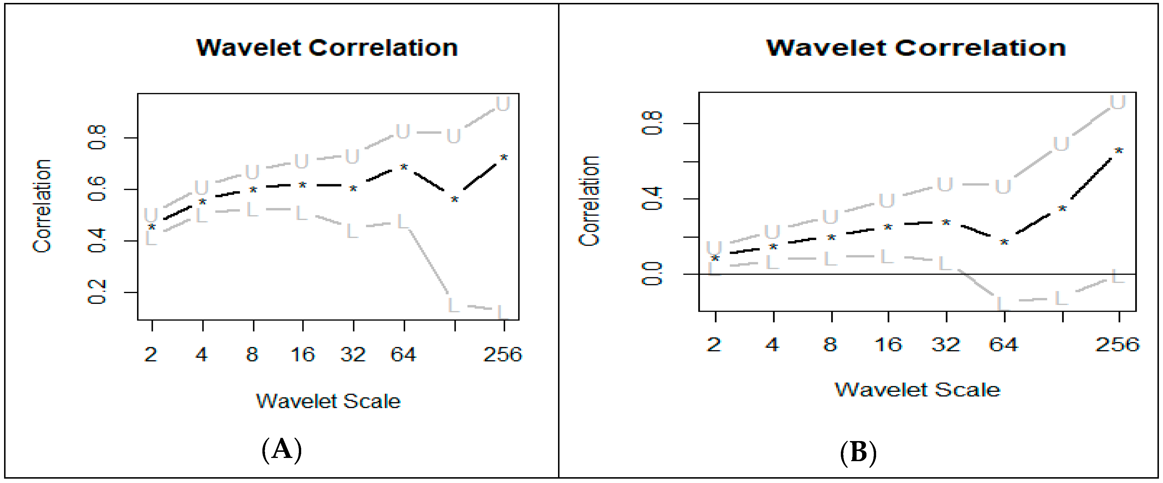
The MODWT analysis carried out in this study applied the Daubechies least asymmetric filter with a filter length of 8 (LA) to investigate financial contagion following the EZDC. The wavelet analysis encompassed 8 scales ranging from 2 days to 18 months, with dyadic increments (2 to 4 days, 4 to 8 days, …, and 256 to 512 days). The scales are displayed on the x axis, while correlations are shown on the y axis. The 95% confidence interval was used to establish statistical significance.
The wavelet analysis revealed significantly positive correlations between the DAX index and the indices of the various BRICS stock markets, with the Chinese market being the only exception. These correlations generally increased with the scale of analysis. A noticeable decline at scale 7 was observable, however (except for the Russian market, which showed a decline at scale 5), with a subsequent rebound at scale 8, where their values became higher than 0.6 (see Figure 1). This suggests that dependencies between the Germany and BRICS equity markets persisted for periods longer than a year. Put differently, the German and BRICS equity markets (excluding the Chinese market) displayed significant correlations over long durations, suggesting a high intensity of mutual influence between these respective markets.
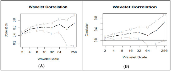
Figure 1.
Correlation of DAX with BOVESPA (panel A) and SSE (panel B) at different timescales. (A) Correlation of DAX and BOVESPA at different time scales. (B) Correlation of DAX and SSE at different time scales.
Figure 1 depicts the wavelet correlation between the DAX index and two individual BRICS indices: the BOVESPA index of Brazil (panel A) and the SSE index of China (panel B). Illustrations for other BRICS indices can be provided upon request from the authors. The lines indicate significant correlations between two time series over specific time scales and locations, with thicker lines indicating stronger correlations. Dashed lines indicate boundaries of 5% confidence intervals, with “L” and “U” mark the lower and upper bounds of the correlation. Asterisks highlight points of significant correlation at particular time or frequency points
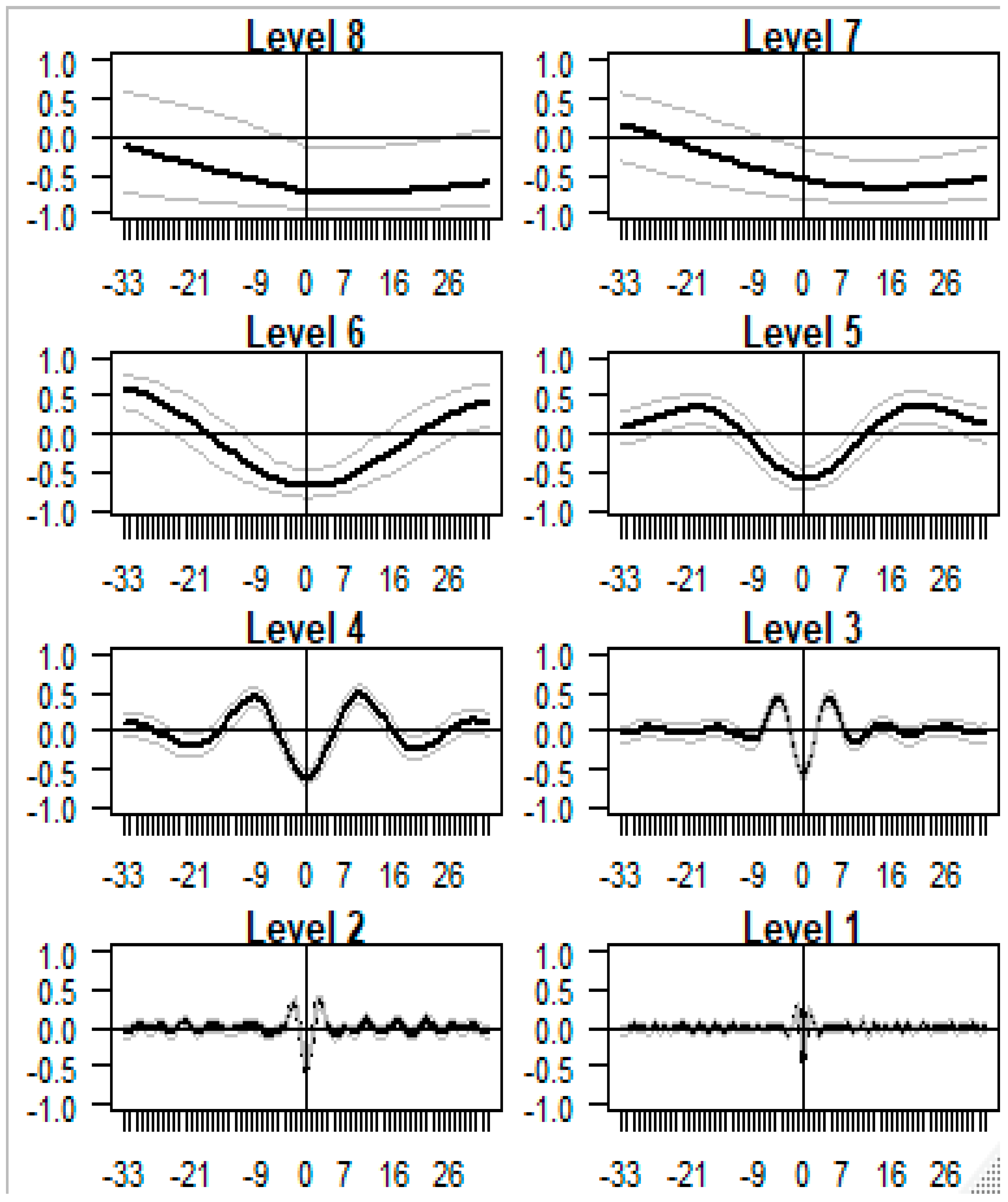
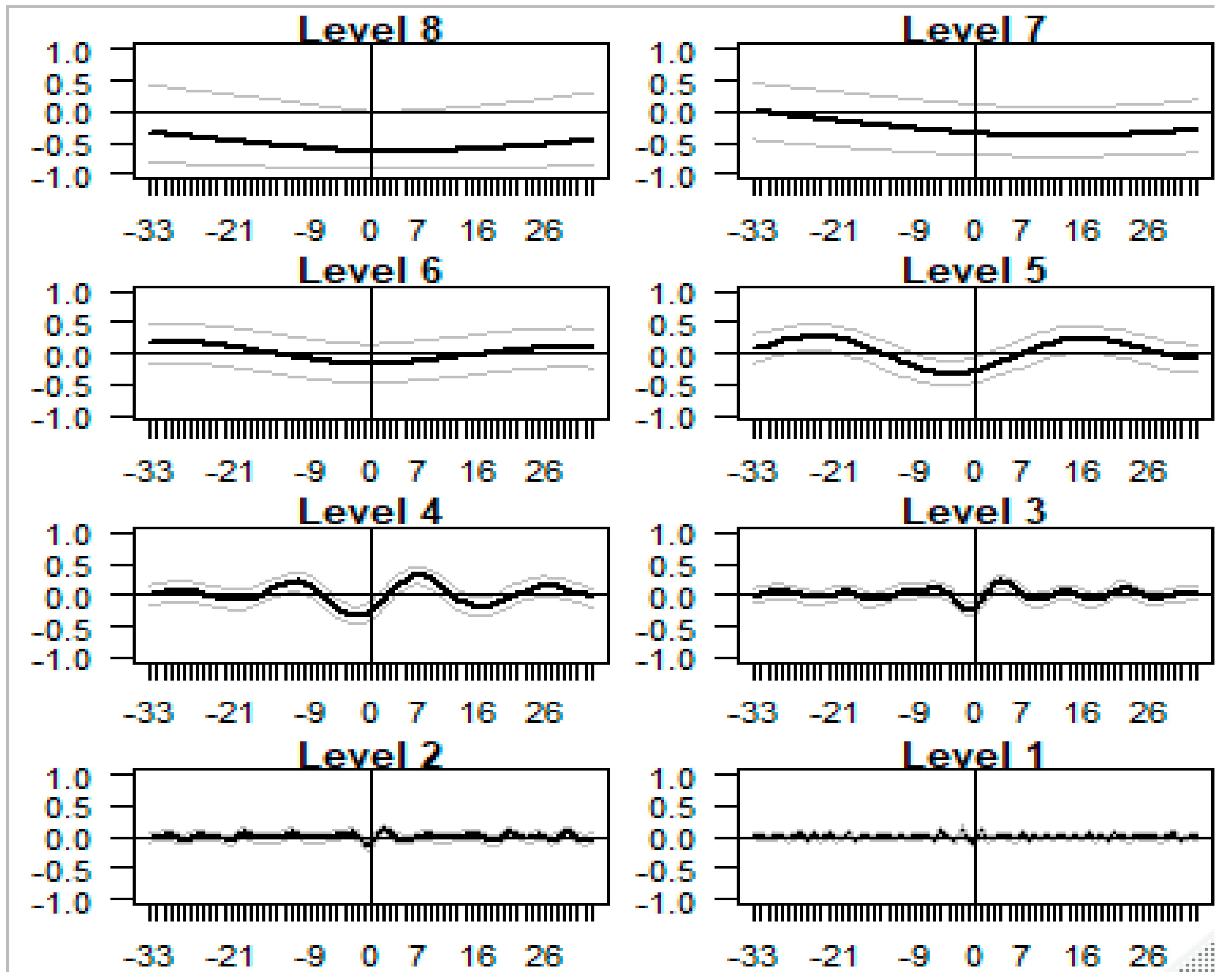
The study also investigated each MODWT pairwise cross-correlation between the DAX index and respective individual BRICS market indices across various wavelet scales ranging from 1 to 33 days. The analysis found positive and significant cross-correlations at the 4 lowest scales, particularly around the time shifts of π = 9 and π = –9. Graphs at these low scales showed a slight right skew, suggesting that the DAX led the individual BRICS indices (see Figure 2 and Figure 3).
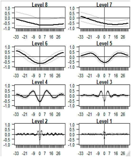
Figure 2.
Cross-correlation between the return series of DAX and BOVESPA.
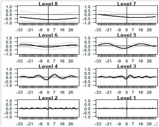
Figure 3.
Cross-correlation between the return series of DAX and SSE.
At scales 5 and 6, the highest correlations were observed around the time shifts of π = 21 and π = −21, although the Chinese stock market showed an exception. Scales 5 and 6 generally exhibited symmetrical distributions, indicating a lack of discernible lead–lag relationships in most cases.
For scale 7, the wavelet cross-correlation was noticeably negative, as can be seen from the graphs of Figure 2 and Figure 32, suggesting that individual BRICS markets led the Eurozone market. Scale 8, however, did not show any clear-cut lead–lag relationship.
Additionally, contemporaneous correlations between the series showed that wavelet correlation coefficients at lag 0 exhibited an anti-correlation relationship. Figure 2 and Figure 3 illustrate cross-correlations between the DAX index and two specific BRICS indices: the BOVESPA index of Brazil and the SSE index of China. Illustrations for other BRICS indices are available upon request from the authors.
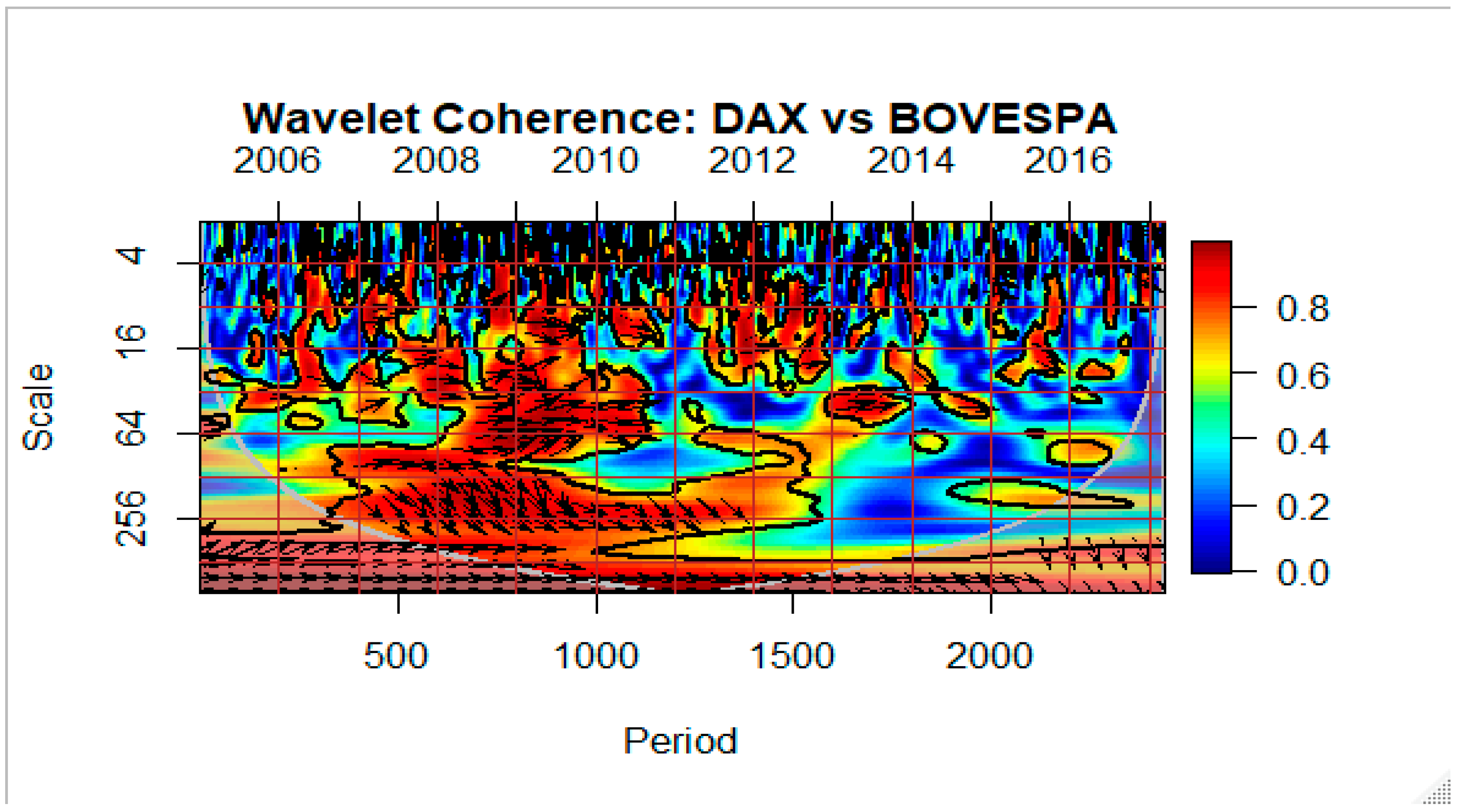
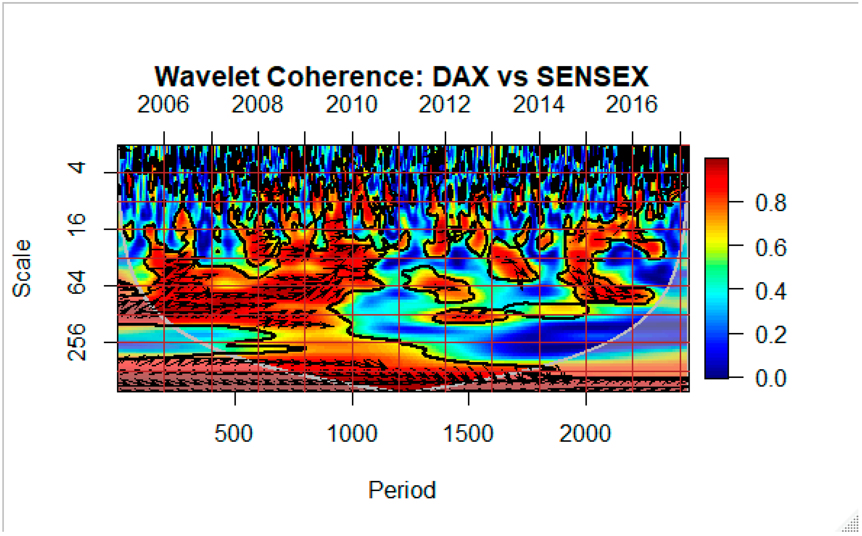
Figure 4, Figure 5, Figure 6, Figure 7 and Figure 8 present wavelet cross-coherence contour plots comparing the DAX index with each BRICS equity market. The horizontal axis shows calendar time, while the vertical axis represents frequency. The thick black line indicates a 5% significance level estimated using Monte Carlo simulation. The white line demarcates the cone of influence, a region influenced by edge effects.
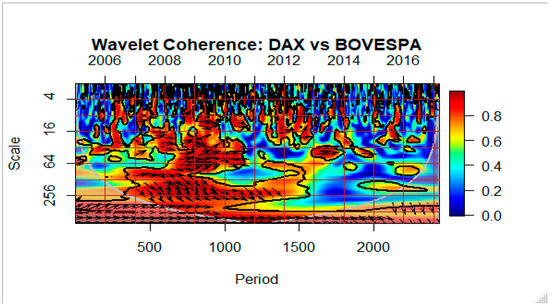
Figure 4.
Wavelet coherence between the Eurozone and Brazilian stock markets. Note: → (pointing to the right): the two time series are in phase and move together; ← (pointing to the left): the two time series are out of phase and move in opposite directions; ↑ (pointing upwards): the first time series leads the second; ↓ (pointing downwards): the second time series leads the first.
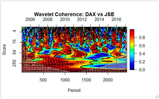
Figure 5.
Wavelet coherence between the Eurozone and South African stock markets. Note: → (pointing to the right): the two time series are in phase and move together; ← (pointing to the left): the two time series are out of phase and move in opposite directions; ↑ (pointing upwards): the first time series (DAX) leads the second (JSE); ↓ (pointing downwards): the second time series leads the first.
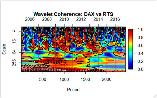
Figure 6.
Wavelet coherence between the Eurozone and Russian stock markets. Note: → (pointing to the right): the two time series are in phase and move together; ← (pointing to the left): the two time series are out of phase and move in opposite directions; ↑ (pointing upwards): the first time series (DAX) leads the second (RTS); ↓ (pointing downwards): the second time series leads the first.

Figure 7.
Wavelet coherence between the Eurozone and Indian stock markets. Note: → (pointing to the right): the two time series are in phase and move together; ← (pointing to the left): the two time series are out of phase and move in opposite directions; ↑ (pointing upwards): the first time series (DAX) leads the second (SENSEX); ↓ (pointing downwards): the second time series leads the first.
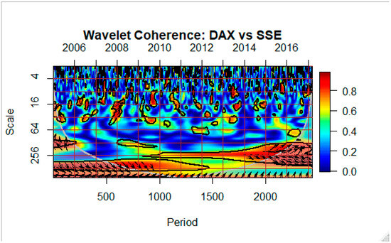
Figure 8.
Wavelet coherence between the Eurozone and Chinese stock markets. Note: → (pointing to the right): the two time series are in phase and move together; ← (pointing to the left): the two time series are out of phase and move in opposite directions; ↑ (pointing upwards): the first time series (DAX) leads the second (SSE); ↓ (pointing downwards): the second time series leads the first.
The heat map, ranging from blue (low coherence) to red (high coherence), represents different levels of correlation. Arrows within the heat map indicate phase relationships:
- Rightward arrows (east): both variables are in phase.
- Leftward arrows (west): variables are out-of-phase.
- Upward arrows (north): the second variable leads the first by 90 degrees.
- Downward arrows (south): the first variable leads the second by 90 degrees.
- Southeast arrows: positive correlation, with the first variable leading.
- Northwest arrows: negative correlation, with the second variable leading.
During the Eurozone crisis (July 2009 to December 2012), most BRICS markets, except China, exhibited higher correlations with the DAX, as indicated by warmer colours. This suggests the presence of contagion, particularly in short-term horizons. Notably, during this period, coherence arrows for most markets pointed southeast, implying a positive correlation, with the DAX leading.
For South Africa and Russia, the southeast-pointing arrows indicated a positive correlation, with the DAX leading. This suggests that changes in the DAX index tended to precede similar movements in the South African JSE and Russian RTS indices. The high correlations observed in short-term horizons are particularly noteworthy, as they strongly suggested the presence of pure contagion. This means that shocks or disturbances in the Eurozone (and more specifically, in the German) market were quickly transmitted to the South African and Russian markets, indicating a high degree of interconnectedness and interdependence.
The strong trading ties between these countries and the Eurozone likely play a significant role in facilitating this contagion. Factors such as trade flows, capital flows, and investor sentiment can all contribute to the transmission of shocks across borders. Until the war in Ukraine started and sanctions were imposed on Russia, South Africa and Russia had strong connections with Germany as important trade partners, with Germany being the third largest export market for South Africa (after China and the US) and the third largest export market for Russian products (after China and the Netherlands). These connections represent sources of interdependencies that may not be directly captured by the structure of financial markets in normal situations but become sources of systemic risk in times of crisis.
In contrast, the contour plots for DAX with BOVESPA, SENSEX, and SSE showed relatively low short-term correlations (Figure 4, Figure 7 and Figure 8). Significant correlations were observed only in the long-term horizon during the Eurozone crisis, suggesting co-movement driven by market fundamentals. Therefore, the study found no evidence of pure contagion in these three countries during the crisis. Our results imply that investors in Brazil, China, and India might have benefited from portfolio diversification during this period due to the limited impact of Eurozone financial contagion. These findings contradict Ahmad et al. (2013), who reported adverse effects on these markets.
It is worth drawing to the reader’s attention that while the MODWT is a particularly robust method that does not necessitate additional robustness checks, it is noteworthy that the data employed in the present study were also utilised in a previous analysis employing the DCC-GARCH model. The DCC-GARCH model corroborated with some of the findings of our current research. The results of these findings were documented by Niyitegeka and Tewari (2021).
5. Conclusions
In evaluating contagion risk, investors should consider non-linear dependencies that extend beyond financial markets, which cannot be easily detected by traditional econometric market correlations. Wavelet analysis provides a suitable tool for denoising the dynamics of financial data and identifying signs of systemic risk and contagion. Policymakers should learn from past experiences to develop optimal policy approaches to insulate their economies from unwanted external volatility.
The present study used the wavelet analysis to examine multiscale interdependence of BRICS equity markets, vis-à-vis the German market as a source country in the aftermath of the EZDC. The results of the wavelet cross-correlation analysis brought to light evidence of co-movement and volatility spillover in the low scales, with the DAX index leading the BRICS market indices. For coarse scales, the wavelet cross-correlation was identified as significantly negative, suggesting that the individual BRICS markets led the Eurozone market.
The wavelet coherence results also provided evidence of high correlation at lower scales between the German stock market and individual stock markets in South Africa and Russia. This is indicative of the presence of financial contagion in these markets. For the Brazilian, Indian, and Chinese stock markets, no correlation was identified in the short-run horizon. This observation led to the conclusion that they suffered no financial contagion induced by the Eurozone crisis. This implies that portfolio diversification could have benefited investors in Brazil, China, and India during the debt crisis, considering the minimal impact of Eurozone financial contagion on these markets.
The study’s limitations include a narrow focus on the DAX index as the sole proxy for the Eurozone, which may not fully capture the region’s financial diversity, and a restricted analysis that omitted a broad range of emerging markets, potentially leading to an incomplete understanding of global financial integration and contagion effects. For future research, we suggest expanding the scope of this analysis in two key directions. Firstly, including more emerging markets could offer valuable insights into regional contagion effects and the extent of global financial integration. This broader perspective would help in understanding how different regions respond to financial shocks and whether similar integration patterns exist elsewhere.
Secondly, while our study used the DAX to probe contagion from the Eurozone market, incorporating additional major European indices, such as the CAC 40 (France) and EURONEXT index, MIB (Italy), could strengthen the analysis and enhance the generalisability of our findings. This more comprehensive representation of the Eurozone would provide a more nuanced understanding of the contagion dynamics between Europe and the emerging countries.
These expansions in future studies would not only build upon our current findings but also contribute to a more robust understanding of global financial interconnectedness and the transmission of economic shocks across diverse markets.
Author Contributions
Conceptualization, O.N. and A.H.; methodology, O.N.; software, O.N.; validation, O.N. and A.H.; formal analysis, O.N.; investigation, A.H.; resources, O.N.; data curation, O.N. and A.H.; writing—original draft preparation, O.N.; writing—review and editing, O.N. and A.H.; visualization, O.N.; supervision, O.N. and A.H.; project administration, O.N. and A.H.; funding acquisition, O.N. and A.H. All authors have read and agreed to the published version of the manuscript.
Funding
This research received no external funding.
Data Availability Statement
The data were sourced from Thomson Reuters Datastream.
Conflicts of Interest
The authors declare no conflicts of interest.
Notes
| 1 | Augmented Dickey–Fuller (ADF), Phillips–Perron (PP), and Kwiatkowski–Phillips–Schmidt–Shin (KPSS) unit root tests were conducted on the data, and all data were found to be stationary. The results of these tests can be provided upon request. |
| 2 | In this wavelet cross-correlation graph, the black line represents the estimated cross-correlation between two time series at various scales, with each level corresponding to a different frequency band. Lower levels capture short-term fluctuations, while higher levels show longer-term trends. The gray lines depict the confidence intervals, helping assess the statistical significance of the correlation. If the black line falls outside the gray lines, the correlation is significant; otherwise, it is not. The horizontal axis indicates time lags, and the vertical axis measures the strength of the correlation, ranging from −1 to 1. |
References
- Abramovich, Felix, Theofanis Sapatinas, and Bernard W. Silverman. 1998. Wavelet thresholding via a Bayesian approach. Journal of the Royal Statistical Society: Series B (Statistical Methodology) 60: 725–49. [Google Scholar] [CrossRef]
- Adrian, Tobias, and Markus K. Brunnermeier. 2011. CoVaR. NBER Working Paper w17454. Cambridge: National Bureau of Economic Research. [Google Scholar]
- Ahmad, Wasim, Sanjay Sehgal, and Nagapudi R. Bhanumurthy. 2013. Eurozone crisis and BRIICKS stock markets: Contagion or market interdependence? Economic Modelling 33: 209–25. [Google Scholar] [CrossRef]
- Akhtaruzzaman, Md, Sabri Boubaker, and Ahmet Sensoy. 2021. Financial contagion during COVID-19 crisis. Finance Research Letters 38: 101604. [Google Scholar] [CrossRef] [PubMed]
- Batondo, Musumba, and Josine Uwilingiye. 2022. Comovement across BRICS and the US Stock Markets: A Multitime Scale Wavelet Analysis. International Journal of Financial Studies 10: 27. [Google Scholar] [CrossRef]
- Benkraiem, Ramzi, Riadh Garfatta, Faten Lakhal, and Imen Zorgati. 2022. Financial contagion intensity during the COVID-19 outbreak: A copula approach. International Review of Financial Analysis 81: 102136. [Google Scholar] [CrossRef]
- Bhar, Ramaprasad, and Biljana Nikolova. 2009. Return, volatility spillovers and dynamic correlation in the BRIC equity markets: An analysis using a bivariate EGARCH framework. Global Finance Journal 19: 203–18. [Google Scholar] [CrossRef]
- Böckelman, Philip. 2020. Timescale-Dependent International Stock Market Co-Movement in the Post-Financial Crisis Decade. Master’s thesis, Hanken School of Economics, Helsinki, Finland. [Google Scholar]
- Chevallier, Julien. 2020. COVID-19 pandemic and financial contagion. Journal of Risk and Financial Management 13: 309. [Google Scholar] [CrossRef]
- Claessens, Stijn, and Kristin Forbes, eds. 2013. International Financial Contagion. Berlin/Heidelberg: Springer Science & Business Media. [Google Scholar]
- Dajčman, Silvo. 2013. Interdependence between some major European stock markets-a wavelet lead/lag analysis. Prague Economic Papers 22: 28–49. [Google Scholar] [CrossRef]
- Dooley, Michael, and Michael Hutchison. 2009. Transmission of the U.S. subprime crisis to emerging markets: Evidence on the decoupling-recoupling hypothesis. Journal of International Money and Finance 28: 1331–49. [Google Scholar] [CrossRef]
- Euronext. 2024. CAC 40®® Index Factsheet. Available online: https://live.euronext.com/en/products/indices/indices-documents-by-family (accessed on 28 June 2024).
- Fröhlich, Stefan. 2021. The Future of the Global Economy and the Euro Area. In The End of Self-Bondage: German Foreign Policy in a World without Leadership. Wiesbaden: Springer, pp. 21–45. [Google Scholar]
- Ganguly, Soumya, and Amalendu Bhunia. 2022. Testing volatility and relationship among BRICS stock market returns. SN Business & Economics 2: 111. [Google Scholar]
- Gelos, Gaston, and Jay Surti. 2016. The growing importance of financial spillovers from emerging market economies. In International Monetary Fund Global Financial Stability Report: Potent Policies for a Successful Normalization. Washington, DC: International Monetary Fund, pp. 57–86. [Google Scholar]
- Gençay, Ramazan, Faruk Selçuk, and Brandon Whitcher. 2003. Systematic risk andtimescales. Quantitative Finance 3: 108. [Google Scholar] [CrossRef]
- Gençay, Ramazan, Nikola Gradojevic, Faruk Selçuk, and Brandon Whitcher. 2010. Asymmetry of information flow between volatilities across time scales. Quantitative Finance 10: 895–915. [Google Scholar] [CrossRef]
- Gunay, Samet, and Gokberk Can. 2022. The source of financial contagion and spillovers: An evaluation of the COVID-19 pandemic and the global financial crisis. PLoS ONE 17: e0261835. [Google Scholar] [CrossRef] [PubMed]
- Gurdgiev, Constantin, and Conor O’Riordan. 2021. A wavelet perspective of crisis contagion between advanced economies and the BRIC markets. Journal of Risk and Financial Management 14: 503. [Google Scholar] [CrossRef]
- Hashim, Khairul Khairiah, and Mansur Masih. 2015. Stock Market Volatility and Exchange Rates: MGARCH-DCC and Wavelet Approaches. Munich: University Library of Munich. [Google Scholar]
- Herman, Alexander, and Alexander Klemm. 2019. Financial deepening in Mexico. Journal of Banking and Financial Economics 1: 5–18. [Google Scholar] [CrossRef]
- In, Francis, and Sangbae Kim. 2013. An Introduction to Wavelet Theory in Finance: A Wavelet Multiscale Approach. London: World Scientific. [Google Scholar]
- Kaminsky, Graciela L., and Carmen M. Reinhart. 2000. On crises, contagion, and confusion. Journal of International Economics 51: 145–68. [Google Scholar] [CrossRef]
- Kannadhasan, Manoharan, and Debojyoti Das. 2019. Has Co-Movement Dynamics in Brazil, Russia, India, China and South Africa (BRICS) Markets Changed after Global Financial Crisis? New Evidence from Wavelet Analysis. Asian Academy of Management Journal of Accounting & Finance 15: 25. [Google Scholar]
- Kenourgios, Dimitris, and Dimitrios Dimitriou. 2015. Contagion of the Global Financial Crisis and the real economy: A regional analysis. Economic Modelling 44: 283–93. [Google Scholar] [CrossRef]
- Kouzehgar, Kamran, and Saeid Eslamian. 2023. Application of experimental data and soft computing techniques in determining the outflow and breach characteristics in embankments and landslide dams. In Handbook of Hydroinformatics. Amsterdam: Elsevier, pp. 11–31. [Google Scholar]
- Kumar, Sanjeev, Reetika Jain, Faruk Narain, Faruk Balli, and Mabruk Billah. 2023. Interconnectivity and investment strategies among commodity prices, cryptocurrencies, and G-20 capital markets: A comparative analysis during COVID-19 and Russian-Ukraine war. International Review of Economics & Finance 88: 547–93. [Google Scholar]
- Muller, Aline, and Willem F. C. Verschoor. 2006. European foreign exchange risk exposure. European Financial Management 12: 195–220. [Google Scholar] [CrossRef]
- Nguyen, Thi Ngan, Thi Kieu Hoa Phan, and Thanh Liem. 2022. Financial contagion during global financial crisis and COVID-19 pandemic: The evidence from DCC–GARCH model. Cogent Economics & Finance 10: 2051824. [Google Scholar]
- Niyitegeka, Olivier, and Devi Datt Tewari. 2021. Bivariate Conditional Heteroscedasticity Model with Dynamic Correlations for Testing Contagion in BRICS Countries. Academy of Accounting and Financial Studies Journal 25: 1–17. [Google Scholar]
- Ozkan, F. Gulcin, and Filiz Unsal. 2012. Global Financial Crisis, Financial Contagion, and Emerging Markets. Washington, DC: International Monetary Fund. [Google Scholar]
- Percival, Donald B., and Andrew T. Walden. 2006. Wavelet Methods for Time Series Analysis. London: Cambridge University Press, vol. 4. [Google Scholar]
- Percival, Donald P. 1995. On estimation of the wavelet variance. Biometrika 83: 619–31. [Google Scholar] [CrossRef]
- Ranta, Mikko. 2010. Wavelet Multiresolution Analysis of Financial Time Series. Unpublished Ph.D. dissertation, University of Vaasa, Vaasa, Finland. [Google Scholar]
- Rigobon, Roberto. 2002. International Financial Contagion: Theory and Evidence in Evolution. Charlottesville: Research Foundation of AIMR. [Google Scholar]
- Ruch, Franz Ulrich. 2020. Prospects, Risks, and Vulnerabilities in Emerging and Developing Economies: Lessons from the Past Decade. World Bank Policy Research Working Paper No. 9181. Washington, DC: World Bank Group. [Google Scholar]
- Saiti, Buerhan, Obiyathulla Ismath Bacha, and Mansur Masih. 2016. Testing the conventional and Islamic financial market contagion: Evidence from wavelet analysis. Emerging Markets Finance and Trade 52: 1832–49. [Google Scholar] [CrossRef]
- Sehgal, Sanjay, Arjun Mittal, and Anand Mittal. 2019. Dynamic linkages between BRICS and other emerging equity markets. Theoretical Economics Letters 9: 2636. [Google Scholar] [CrossRef]
- Syllignakis, Manolis N., and Georgios P. Kouretas. 2011. Dynamic correlation analysis of financial contagion: Evidence from the Central and Eastern European markets. International Review of Economics and Finance 20: 717–32. [Google Scholar] [CrossRef]
- Torrence, Christopher, and Gilbert P. Compo. 1998. A practical guide to wavelet analysis. Bulletin of the American Meteorological Society 79: 61–78. [Google Scholar] [CrossRef]
- Trešl, Jiří, and Dagmar Blatná. 2007. Dynamic analysis of selected European stock markets. Prague Economic Papers 16: 291–302. [Google Scholar] [CrossRef]
- Wilks, Daniel S. 2020. Statistical Methods in the Atmospheric Sciences, 4th ed. Amsterdam: Elsevier. [Google Scholar]
- Xiao, Fei, Tianguang Lu, Mingli Wu, and Qian Ai. 2020. Maximal overlap discrete wavelet transform and deep learning for robust denoising and detection of power quality disturbance. IET Generation, Transmission & Distribution 14: 140–47. [Google Scholar]
- Yiu, Matthew S., Wai-Yip Alex Ho, and Daniel F. Choi. 2010. Dynamic correlation analysis of financial contagion in Asian markets in global financial turmoil. Applied Financial Economics 20: 345–54. [Google Scholar] [CrossRef]


Disclaimer/Publisher’s Note: The statements, opinions and data contained in all publications are solely those of the individual author(s) and contributor(s) and not of MDPI and/or the editor(s). MDPI and/or the editor(s) disclaim responsibility for any injury to people or property resulting from any ideas, methods, instructions or products referred to in the content. |
© 2024 by the authors. Licensee MDPI, Basel, Switzerland. This article is an open access article distributed under the terms and conditions of the Creative Commons Attribution (CC BY) license (https://creativecommons.org/licenses/by/4.0/).