
Credit Card Default Prediction: An Empirical Analysis on Predictive Performance Using Statistical and Machine Learning Methods


Abstract
1. Introduction
2. Literature Review
3. Materials and Methods
3.1. Linear Discriminant Analysis
3.2. Logistic Regression
3.3. Support Vector Machine
3.4. XGBoost
3.5. Random Forest Classifier
3.6. Deep Neural Network
Deep Neural Network Architecture
3.7. Methodology
4. Results
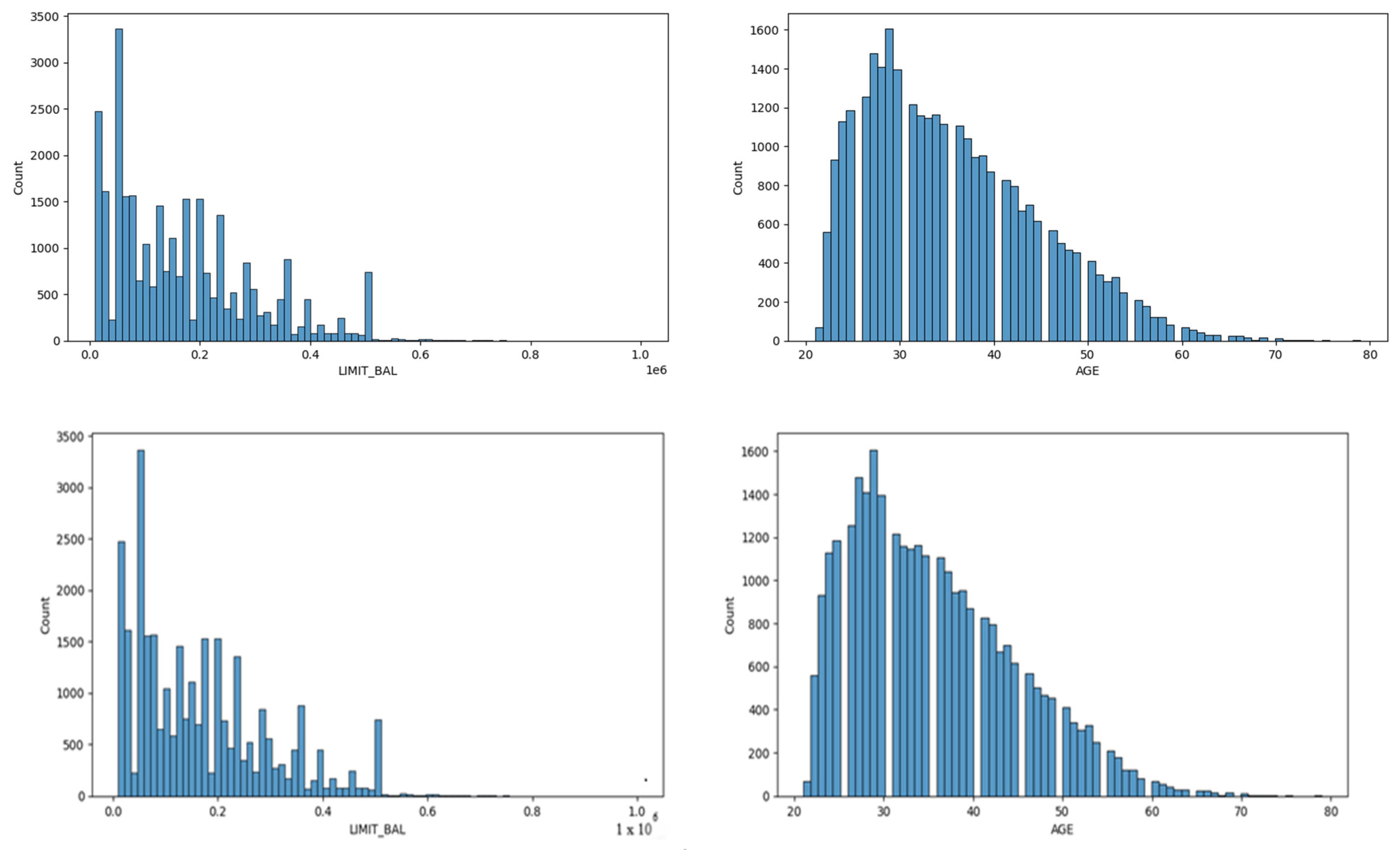
4.1. Descriptives
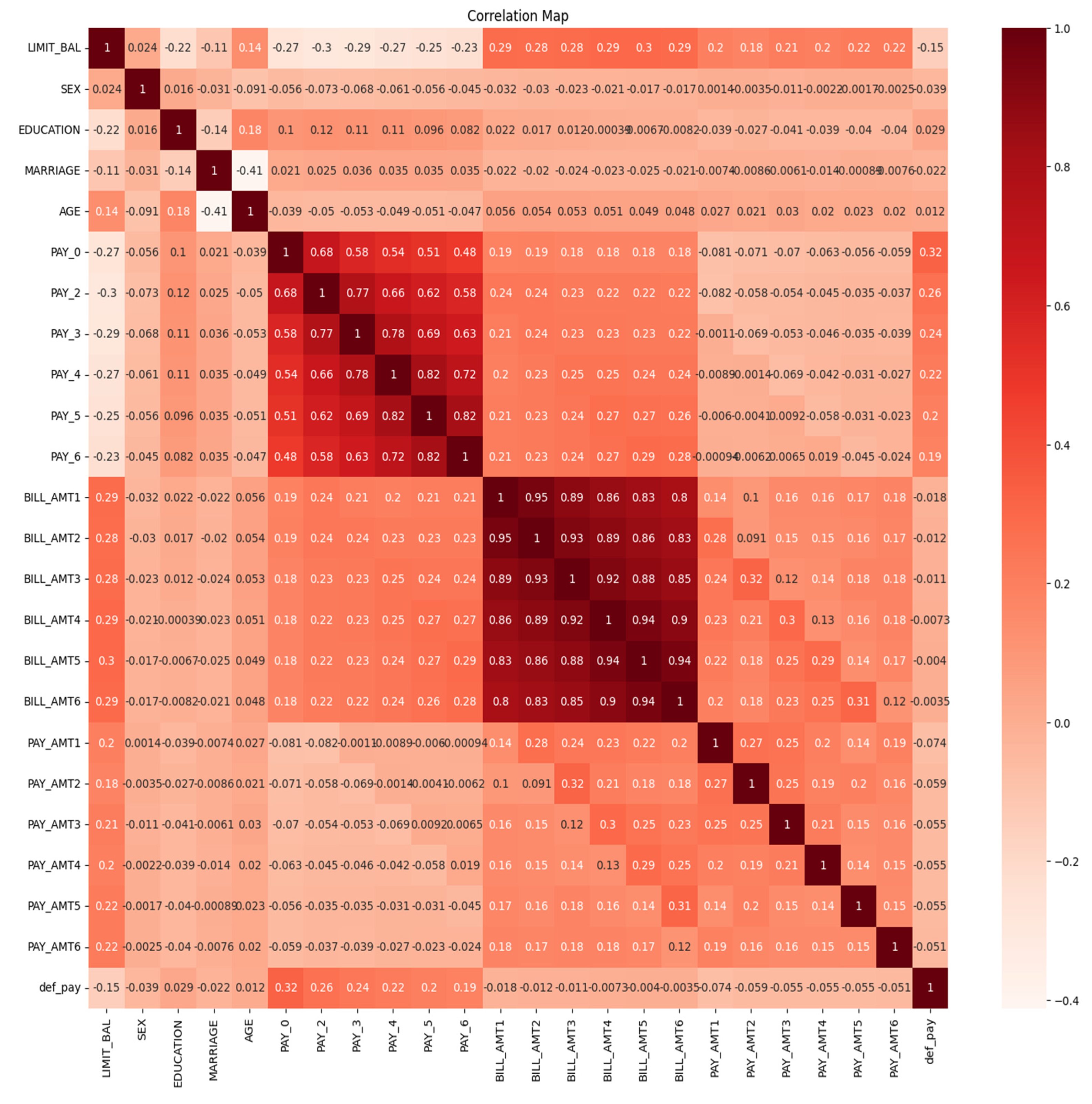
4.2. Heat Map
4.3. Confusion Matrix Analysis
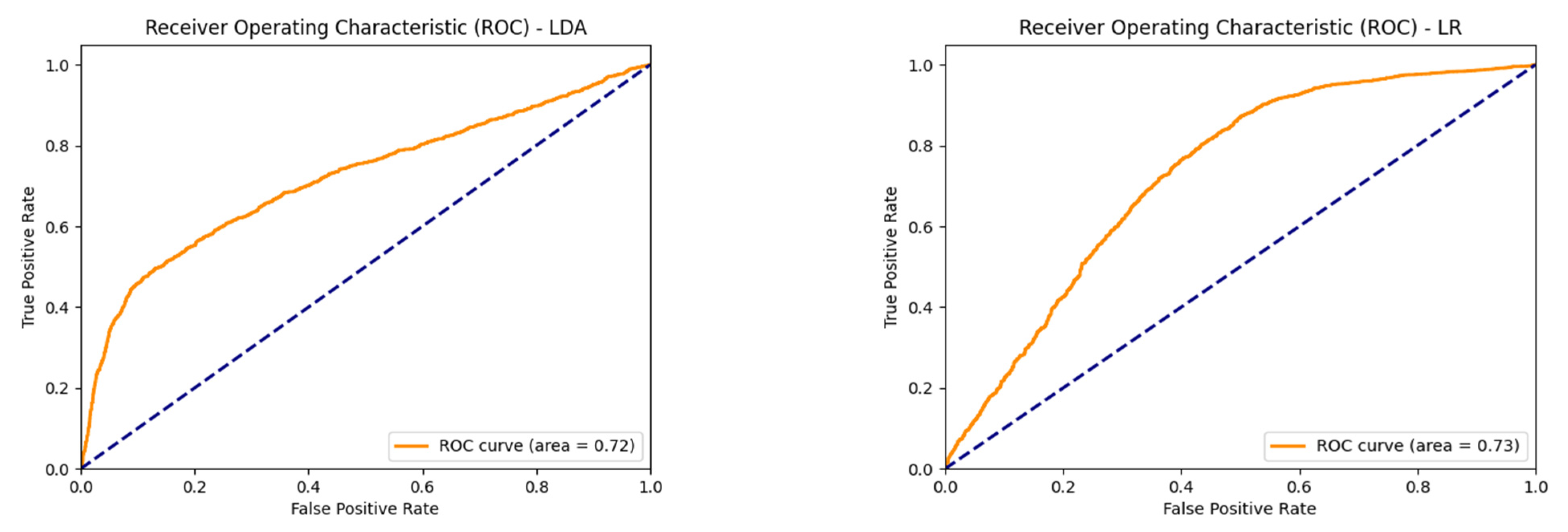
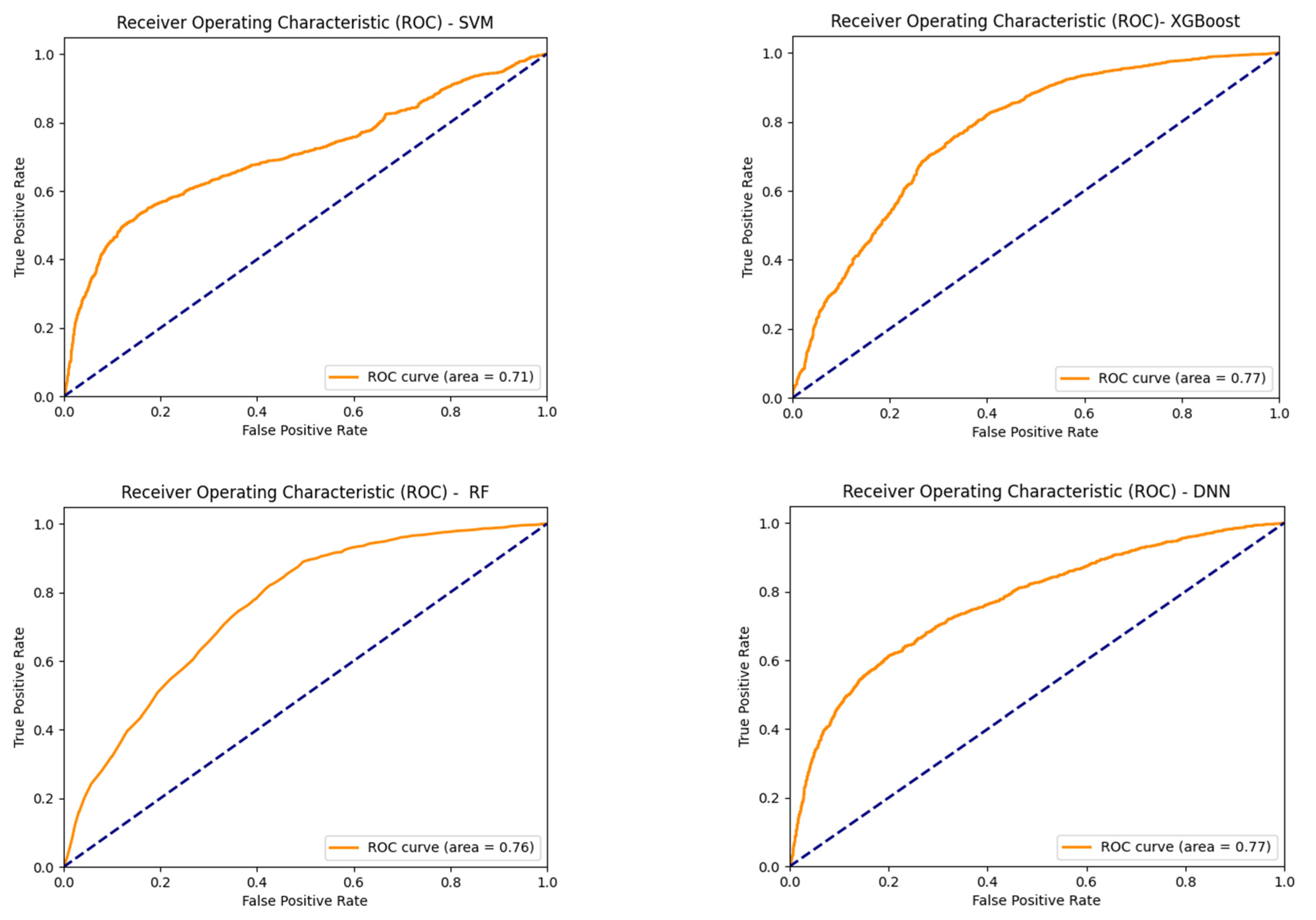
4.4. Receiver Operating Characteristics (ROCs)
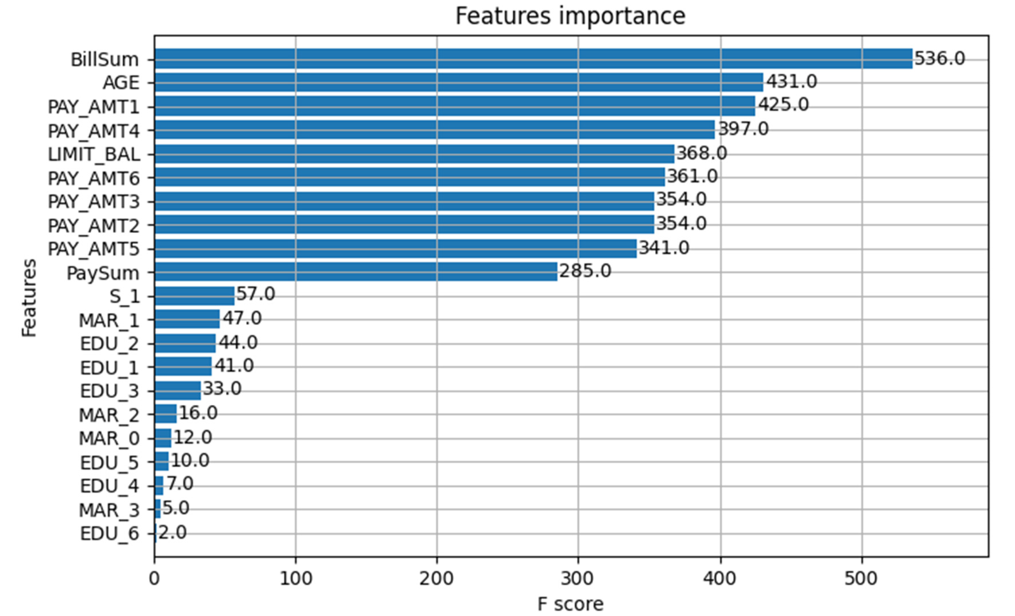
4.5. Feature Importance
4.6. Default Score Calculation
5. Discussions and Implications
6. Conclusions
Author Contributions
Funding
Institutional Review Board Statement
Informed Consent Statement
Data Availability Statement
Conflicts of Interest
References
- Acquah, H. D., & Addo, J. (2011). Determinants of loan repayment performance of fishermen: Empirical evidence from Ghana. Cercetari Agronomice in Moldova, 44(4), 89–97. [Google Scholar]
- Addisu, M. (2006). Micro-finance repayment problems in the informal sector in Addis Ababa. Ethiopian Journal of Business & Development, 1(2), 29–50. [Google Scholar]
- Baesens, B., Setiono, R., Mues, C., & Vanthienen, J. (2003). Using neural network rule extraction and decision tables for credit-risk evaluation. Management Science, 49(3), 312–329. [Google Scholar] [CrossRef]
- Bali, T. G., Beckmeyer, H., Mörke, M., & Weigert, F. (2023). Option return predictability with machine learning and big data. The Review of Financial Studies, 36(9), 3548–3602. [Google Scholar] [CrossRef]
- Bandyopadhyay, A. (2023). Predicting the probability of default for banks’ expected credit loss provisions. Economic & Political Weekly, 58(10), 15–19. [Google Scholar]
- Bastos, J. A. (2010). Forecasting bank loans loss-given-default. Journal of Banking & Finance, 34(10), 2510–2517. [Google Scholar] [CrossRef]
- Bazarbash, M. (2019). Fintech in financial inclusion: Machine learning applications in assessing credit risk. International Monetary Fund. [Google Scholar]
- Bekkar, M., Kheliouane Djemaa, H., & Akrouf Alitouche, T. (2013). Evaluation measures for models assessment over imbalanced data sets. Journal of Information Engineering and Applications, 3(10), 27–38. [Google Scholar]
- Bellotti, A., Brigo, D., Gambetti, P., & Vrins, F. (2021). Forecasting recovery rates on non-performing loans with machine learning. International Journal of Forecasting, 37(1), 428–444. [Google Scholar] [CrossRef]
- Bewick, V., Cheek, L., & Ball, J. (2004). Statistics review 13: Receiver operating characteristic curves. Critical Care, 8, 1–5. [Google Scholar]
- Bhandary, R., Shenoy, S. S., Shetty, A., & Shetty, A. D. (2023a). Attitudes toward educational loan repayment among college students: A qualitative enquiry. Journal of Financial Counseling and Planning, 34(2), 281–292. [Google Scholar] [CrossRef]
- Bhandary, R., Shenoy, S. S., Shetty, A., & Shetty, A. D. (2023b). Education loan repayment: A systematic literature review. Journal of Financial Services Marketing, 29, 1365–1376. [Google Scholar] [CrossRef]
- Breiman, L. (2001a). Random forests. Machine Learning, 45, 5–32. [Google Scholar] [CrossRef]
- Breiman, L. (2001b). Statistical modeling: The two cultures (with comments and a rejoinder by the author). Statistical Science, 16(3), 199–231. [Google Scholar] [CrossRef]
- Brown, C. D., & Davis, H. T. (2006). Receiver operating characteristics curves and related decision measures: A tutorial. Chemometrics and Intelligent Laboratory Systems, 80(1), 24–38. [Google Scholar] [CrossRef]
- Cervantes, J., Garcia-Lamont, F., Rodríguez-Mazahua, L., & Lopez, A. (2020). A comprehensive survey on support vector machine classification: Applications, challenges and trends. Neurocomputing, 408, 189–215. [Google Scholar] [CrossRef]
- Chang, C. -H. (2022). Information asymmetry and card debt crisis in taiwan. Bulletin of Applied Economics, 9(2), 123–145. [Google Scholar] [CrossRef]
- Chen, T., & Guestrin, C. (2016, August 13–17). XGBoost. 22nd ACM SIGKDD International Conference on Knowledge Discovery and Data Mining (pp. 785–794), San Francisco, CA, USA. [Google Scholar] [CrossRef]
- Chiang, W. K., Zhang, D., & Zhou, L. (2006). Predicting and explaining patronage behavior toward web and traditional stores using neural networks: A comparative analysis with logistic regression. Decision Support Systems, 41(2), 514–531. [Google Scholar] [CrossRef]
- Coşer, A., Maer-Matei, M. M., & Albu, C. (2019). Predictive models for loan default risk assessment. Economic Computation & Economic Cybernetics Studies & Research, 53(2), 149–165. [Google Scholar] [CrossRef]
- DeVaney, S. A. (1999). Determinants of consumer’s debt repayment patterns. Consumer Interests Annual, 45, 65–70. [Google Scholar]
- Dicon, H. (2024, May 8). Why are americans cutting back on credit card debt? Investopedia. Available online: https://www.investopedia.com/why-americans-are-cutting-back-on-credit-card-debt-8645241 (accessed on 12 September 2024).
- Drobetz, W., & Otto, T. (2021). Empirical asset pricing via machine learning: Evidence from the European stock market. Journal of Asset Management, 22(7), 507–538. [Google Scholar] [CrossRef]
- Fisher, R. A. (1936). The use of multiple measurements in taxonomic problems. Annals of Eugenics, 7(2), 179–188. [Google Scholar] [CrossRef]
- García, S., Luengo, J., & Herrera, F. (2015). Data preprocessing in data mining (Vol. 72, pp. 59–139). Springer International Publishing. [Google Scholar]
- Gauthier, C., Lehar, A., & Souissi, M. (2012). Macroprudential capital requirements and systemic risk. Journal of Financial Intermediation, 21(4), 594–618. [Google Scholar] [CrossRef]
- Géron, A. (2022). Hands-on machine learning with Scikit-Learn, Keras, and TensorFlow. O’Reilly Media, Inc. [Google Scholar]
- Globaldata. (2023). Taiwan cards and payments market report overview. Globaldata Report Store. GDFS0736CI-ST. [Google Scholar]
- Gu, S., Kelly, B., & Xiu, D. (2020). Empirical asset pricing via machine learning. The Review of Financial Studies, 33(5), 2223–2273. [Google Scholar] [CrossRef]
- Gu, Z. (2022). Complex heatmap visualization. Imeta, 1(3), e43. [Google Scholar] [CrossRef]
- Gu, Z., Eils, R., & Schlesner, M. (2016). Complex heatmaps reveal patterns and correlations in multidimensional genomic data. Bioinformatics, 32(18), 2847–2849. [Google Scholar] [CrossRef] [PubMed]
- Hamdi, M., Mestiri, S., & Arbi, A. (2024). Artificial intelligence techniques for bankruptcy prediction of tunisian companies: An application of machine learning and deep learning-based models. Journal of Risk and Financial Management, 17(4), 132. [Google Scholar] [CrossRef]
- Hand, D. J., & Henley, W. E. (1997). Statistical classification methods in consumer credit scoring: A review. Journal of the Royal Statistical Society, Series A–Statistics in Society, 160(3), 523–541. [Google Scholar] [CrossRef]
- Hearst, M. A., Dumais, S. T., Osuna, E., Platt, J., & Scholkopf, B. (1998). Support vector machines. IEEE Intelligent Systems and Their Applications, 13(4), 18–28. [Google Scholar] [CrossRef]
- Hochreiter, S., Younger, A. S., & Conwell, P. R. (2001, August 21–25). Learning to learn using gradient descent. Artificial Neural Networks—ICANN 2001: International Conference, Proceedings 11 (pp. 87–94), Vienna, Austria. [Google Scholar]
- Hubbard, D. W. (2020). The failure of risk management: Why it’s broken and how to fix it. John Wiley & Sons. [Google Scholar]
- IASB—International Accounting Standards Board. (2014). IFRS 9 financial instruments. Available online: http://www.ifrs.org (accessed on 12 September 2024).
- Jayadev, M., Shah, N., & Vadlamani, R. (2019). Predicting educational loan defaults: Application of machine learning and deep learning models. IIM Bangalore Research Paper, 601, 1–46. [Google Scholar]
- Karatas, G., Demir, O., & Sahingoz, O. K. (2020). Increasing the performance of machine learning-based IDSs on an imbalanced and up-to-date dataset. IEEE Access, 8, 32150–32162. [Google Scholar] [CrossRef]
- Krenker, A., Bešter, J., & Kos, A. (2011). Introduction to the artificial neural networks. In Artificial Neural Networks: Methodological Advances and Biomedical Applications (Volume 1, pp. 1–18). InTech. [Google Scholar]
- Kuhn, M., & Johnson, K. (2013). Measuring performance in classification models. In Applied predictive modeling. Springer. [Google Scholar]
- Luque, A., Carrasco, A., Martín, A., & de Las Heras, A. (2019). The impact of class imbalance in classification performance metrics based on the binary confusion matrix. Pattern Recognition, 91, 216–231. [Google Scholar] [CrossRef]
- Maalouf, M. (2011). Logistic regression in data analysis: An overview. International Journal of Data Analysis Techniques and Strategies, 3(3), 281–299. [Google Scholar] [CrossRef]
- Maehara, R., Benites, L., Talavera, A., Aybar-Flores, A., & Muñoz, M. (2024). Predicting financial inclusion in peru: Application of machine learning algorithms. Journal of Risk and Financial Management, 17(1), 34. [Google Scholar] [CrossRef]
- McCulloch, W. S., & Pitts, W. (1943). A logical calculus of the ideas immanent in nervous activity. The Bulletin of Mathematical Biophysics, 5, 115–133. [Google Scholar] [CrossRef]
- More, A. S., & Rana, D. P. (2017, October 5–6). Review of random forest classification techniques to resolve data imbalance. 2017 1st INTERNATIONAL Conference on Intelligent Systems and Information Management (ICISIM) (pp. 72–78), Aurangabad, India. [Google Scholar]
- Musolf, A. M., Holzinger, E. R., Malley, J. D., & Bailey-Wilson, J. E. (2022). What makes a good prediction? Feature importance and beginning to open the black box of machine learning in genetics. Human Genetics, 141(9), 1515–1528. [Google Scholar] [CrossRef] [PubMed]
- Netzer, O., Lemaire, A., & Herzenstein, M. (2019). When words sweat: Identifying signals for loan default in the text of loan applications. Journal of Marketing Research, 56(6), 960–980. [Google Scholar] [CrossRef]
- Nti, I. K., Nyarko-Boateng, O., & Aning, J. (2021). Performance of machine learning algorithms with different K Values in K-fold crossvalidation. International Journal of Information Technology and Computer Science, 13(6), 61–71. [Google Scholar] [CrossRef]
- Ofori, K. S., Fianu, E., Omoregie, O. K., Odai, N. A., & Oduro-Gyimah, F. (2014). Predicting credit default among micro borrowers in Ghana. Research Journal of Finance and Accounting ISSN, 1697–2222. [Google Scholar]
- Puli, S., Thota, N., & Subrahmanyam, A. C. V. (2024). Assessing machine learning techniques for predicting banking crises in India. Journal of Risk and Financial Management, 17(4), 141. [Google Scholar] [CrossRef]
- Ramraj, S., Uzir, N., Sunil, R., & Banerjee, S. (2016). Experimenting XGBoost algorithm for prediction and classification of different datasets. International Journal of Control Theory and Applications, 9(40), 651–662. [Google Scholar]
- Saraiva, A. (2024, August 8). US Consumer Borrowing Rises Less Than Forecast on Credit Cards. Bloomberg. Available online: https://www.bloomberg.com/news/articles/2024-08-07/us-consumer-credit-misses-forecast-on-lower-card-balances (accessed on 12 September 2024).
- Schreiner, M. (2000). Credit scoring for microfinance: Can it work. Journal of Microfinance/ESR Review, 2(2), 105–118. [Google Scholar]
- Shao, Y., Ahmed, A., Zamrini, E. Y., Cheng, Y., Goulet, J. L., & Zeng-Treitler, Q. (2023). Enhancing clinical data analysis by explaining interaction effects between covariates in deep neural network models. Journal of Personalized Medicine, 13(2), 217. [Google Scholar] [CrossRef]
- Sperandei, S. (2014). Understanding logistic regression analysis. Biochemia Medica, 12–18. [Google Scholar] [CrossRef] [PubMed]
- Suhadolnik, N., Ueyama, J., & Da Silva, S. (2023). Machine learning for enhanced credit risk assessment: An empirical approach. Journal of Risk and Financial Management, 16(12), 496. [Google Scholar] [CrossRef]
- Sze, V., Chen, Y. H., Yang, T. J., & Emer, J. S. (2017). Efficient processing of deep neural networks: A tutorial and survey. Proceedings of the IEEE, 105(12), 2295–2329. [Google Scholar] [CrossRef]
- Tharwat, A., Gaber, T., Ibrahim, A., & Hassanien, A. E. (2017). Linear discriminant analysis: A detailed tutorial. AI communications, 30(2), 169–190. [Google Scholar] [CrossRef]
- Thomas, L. C., Matuszyk, A., So, M. C., Mues, C., & Moore, A. (2016). Modelling repayment patterns in the collections process for unsecured consumer debt: A case study. European Journal of Operational Research, 249(2), 476–486. [Google Scholar] [CrossRef]
- Vapnik, V. (1998). The support vector method of function estimation. In Nonlinear modeling: Advanced black-box techniques (pp. 55–85). Springer. [Google Scholar]
- Varian, H. R. (2014). Big data: New tricks for econometrics. Journal of Economic Perspectives, 28(2), 3–28. [Google Scholar] [CrossRef]
- Viswanathan, P. K., & Shanthi, S. K. (2017). Modelling credit default in microfinance—an indian case study. Journal of Emerging Market Finance, 16(3), 246–258. [Google Scholar] [CrossRef]
- Yeh, I. -C. (2016). Default of credit card clients. UCI Machine Learning Repository, 10, C55S3H. [Google Scholar]
- Yeh, I. C., & Lien, C. H. (2009). The comparisons of data mining techniques for the predictive accuracy of probability of default of credit card clients. Expert Systems with Applications, 36(2), 2473–2480. [Google Scholar] [CrossRef]
- Zheng, A., & Casari, A. (2018). Feature engineering for machine learning: Principles and techniques for data scientists. O’Reilly Media, Inc. [Google Scholar]


| Feature ID | Feature Code | Description |
|---|---|---|
| X1 | Limit_bal | The amount of credit that the card holder is entitled to avail. It includes individual and family credit. |
| X2 | Sex | (Gender) 1 = male, 2 = female |
| X3 | Education | 1 = graduate, 2 = university, 3 = high school, 4 = others |
| X4 | Marital status | 1 = married, 2 = single, 3 = others |
| X5 | Age | 21 years to 79 years |
| X6 to X11 | Repayment status codes −1 = paid duly 1 = payment delay for one month 2 = payment delay for two months ….. 9 = payment delay for 9 months and above | History of past payment month-wise X6 = repayment status for the month of September 2005 X7 = repayment status for the month of August 2005 X8 = repayment status for the month of July 2005 X9 = repayment status for the month of June 2005 X10 = repayment status for the month of May 2005 X11 = repayment status for the month of April 2005 |
| X12 to X17 | Amount of bill statement | X12 = amount of bill statement for September 2005 X13 = amount of bill statement for August 2005 X14 = amount of bill statement for July 2005 X15 = amount of bill statement for June 2005 X16 = amount of bill statement for May 2005 X17 = amount of bill statement for April 2005 |
| X18 to X23 | Amount of previous payment | X18 = amount paid in September 2005 X19 = amount paid in August 2005 X20 = amount paid in July 2005 X21 = amount paid in June 2005 X22 = amount paid in May 2005 X23 = amount paid in April 2005 |
| Actual | Prediction | |
|---|---|---|
| 0 (Negative) | 1 (Positive) | |
| 0 (negative) | True negative (TN) | False positive (FP) |
| 1 (positive) | False negative (FN) | True positive (TP) |
| Metric | Formula |
|---|---|
| Accuracy | |
| Error rate = 1 – accuracy | |
| Sensitivity (or recall, accuracy of positive examples) | |
| Specificity (accuracy of negative examples) | |
| Prescision | |
| F1 score | 2 × |
| G-mean |
| LDA | LR | SVM | ||||||
| Actual | Prediction | Actual | Prediction | Actual | Prediction | |||
| 0 | 1 | 0 | 1 | 0 | 1 | |||
| 0 | 4529 | 158 | 0 | 4549 | 138 | 0 | 4560 | 127 |
| 1 | 988 | 325 | 1 | 1002 | 311 | 1 | 1010 | 303 |
| XGBoost | RF | DNN | ||||||
| Actual | Prediction | Actual | Prediction | Actual | Prediction | |||
| 0 | 1 | 0 | 1 | 0 | 1 | |||
| 0 | 4406 | 281 | 0 | 4417 | 270 | 0 | 4400 | 287 |
| 1 | 819 | 494 | 1 | 832 | 481 | 1 | 805 | 508 |
| Mertric | LDA | LR | SVM | XGBoost | RF | DNN |
|---|---|---|---|---|---|---|
| Accuracy | 0.8090 | 0.8100 | 0.8105 | 0.8167 | 0.8163 | 0.8180 |
| Sensitivity or recall | 0.2475 | 0.2369 | 0.2308 | 0.3762 | 0.3663 | 0.3869 |
| Specifivity | 0.9663 | 0.9706 | 0.9729 | 0.9400 | 0.9424 | 0.9388 |
| Precision | 0.6729 | 0.6927 | 0.7047 | 0.6374 | 0.6405 | 0.6390 |
| F1 score | 0.3619 | 0.3530 | 0.3477 | 0.4732 | 0.4661 | 0.4820 |
| G-mean | 0.4891 | 0.4794 | 0.4738 | 0.5947 | 0.5876 | 0.6027 |
| AUC | 0.72 | 0.73 | 0.71 | 0.77 | 0.76 | 0.77 |
Disclaimer/Publisher’s Note: The statements, opinions and data contained in all publications are solely those of the individual author(s) and contributor(s) and not of MDPI and/or the editor(s). MDPI and/or the editor(s) disclaim responsibility for any injury to people or property resulting from any ideas, methods, instructions or products referred to in the content. |
© 2025 by the authors. Licensee MDPI, Basel, Switzerland. This article is an open access article distributed under the terms and conditions of the Creative Commons Attribution (CC BY) license (https://creativecommons.org/licenses/by/4.0/).
Share and Cite
Bhandary, R.; Ghosh, B.K. Credit Card Default Prediction: An Empirical Analysis on Predictive Performance Using Statistical and Machine Learning Methods. J. Risk Financial Manag. 2025, 18, 23. https://doi.org/10.3390/jrfm18010023
Bhandary R, Ghosh BK. Credit Card Default Prediction: An Empirical Analysis on Predictive Performance Using Statistical and Machine Learning Methods. Journal of Risk and Financial Management. 2025; 18(1):23. https://doi.org/10.3390/jrfm18010023
Chicago/Turabian StyleBhandary, Rakshith, and Bidyut Kumar Ghosh. 2025. "Credit Card Default Prediction: An Empirical Analysis on Predictive Performance Using Statistical and Machine Learning Methods" Journal of Risk and Financial Management 18, no. 1: 23. https://doi.org/10.3390/jrfm18010023
APA StyleBhandary, R., & Ghosh, B. K. (2025). Credit Card Default Prediction: An Empirical Analysis on Predictive Performance Using Statistical and Machine Learning Methods. Journal of Risk and Financial Management, 18(1), 23. https://doi.org/10.3390/jrfm18010023