Abstract
Loan defaults have become an increasing concern for lending institutions, presenting significant challenges to profitability and operational stability. However, with the advent of advanced data processing capabilities, greater data availability, and the development of sophisticated machine learning techniques—particularly neural networks—new opportunities have emerged for classifying and predicting loan defaults beyond traditional manual methods. This, in turn, can reduce risk and enhance overall financial performance. In recent years, institutions have increasingly employed these advanced techniques to mitigate the risk of non-performing loans (NPLs) by improving loan approval efficiency. This study aims to address a gap in the literature by examining the predictive performance of different neural network architectures on financial loan datasets. Specifically, it compares the effectiveness of Feedforward Neural Networks (FNNs), Long Short-Term Memory (LSTM) networks, and one-dimensional Convolutional Neural Networks (1D-CNNs) in forecasting loan defaults. Despite the growing body of research in this area, comparative studies focusing on the application of various neural network techniques to loan default prediction remain relatively scarce.
1. Introduction
Many factors can directly or indirectly influence the rate of loan defaults. Croux et al. (2020) emphasized the importance of various contractual loan features, borrower characteristics, and macroeconomic variables—such as loan maturity, ownership status, loan purpose, and occupational background—in determining the likelihood of default. They advocated for greater transparency, enhanced risk assessment practices, and the use of alternative data sources to improve the prediction of default rates. Researchers such as Lai (2020) and Wang and Perkins (2019) have highlighted the transformative potential of machine learning in credit analysis, arguing that the combination of advanced algorithms and vast datasets enables lending institutions to build more robust and accurate models for identifying potential defaulters. Wang and Perkins (2019) highlighted additional factors, such as borrowers’ local economic conditions (e.g., unemployment rates), which can significantly influence the realized outcome of a loan.
While much research has focused on the importance of accurate credit risk prediction to improve the financial performance of lending institutions, another crucial area of inquiry is the advancement of predictive algorithms. Historically, researchers have relied on parametric approaches such as regression, logistic regression, and linear discriminant analysis for financial modelling (Beaver, 1966; Altman, 1968; Black & Scholes, 1973). Among these, Logit Regression (LR) and Multivariate Discriminant Analysis (MDA) were the most commonly used statistical models. However, these models depend heavily on assumptions that are often violated due to the complex and non-linear nature of financial data. Acknowledging these limitations, researchers across disciplines, including in financial risk, have increasingly turned to more flexible, data-driven approaches.
The 1990s marked a pivotal shift away from traditional parametric methods. During this period, advanced techniques such as Feedforward Neural Networks (also known as Multi-Layer Perceptrons or MLPs) began to be rigorously compared to conventional models. Due to their simplicity and promising early results, MLPs gained traction, leading to further advancements in neural network architectures. Today, variants such as MLPs, Recurrent Neural Networks (RNNs), and Convolutional Neural Networks (CNNs) have become mainstream, particularly in applications that require modelling non-linear relationships between variables. In fields, such as life sciences, finance, transportation, and energy, the demand for predictive modelling, such as housing price forecasts, has shifted away from traditional methods toward machine learning techniques, especially neural networks.
In the existing literature, comparisons between traditional models (both parametric and non-parametric) and single neural network architectures are common. However, comprehensive studies comparing multiple neural network architectures applied to loan default prediction remain limited.
This research contributes to the literature in the following key ways:
- Comparative Evaluation of Model Performance:
- We assess the influence of data characteristics (e.g., sparse vs. dense, temporal vs. non-temporal) on the performance of various algorithms, including Support Vector Machines (SVMs), Gradient Boosting, XGBoost, LightGBM, and several neural network models. The neural network architectures examined include Feedforward Neural Networks (FNNs/MLP), Long Short-Term Memory (LSTM), and 1D Convolutional Neural Networks (1D-CNNs).
- Assessment of Architecture Suitability:
- We explore the suitability of each neural network architecture based on data characteristics, aiming to generalize their effectiveness in different contexts. For example, we compare the performance of 1D-CNNs and FNNs on smaller datasets containing categorical features, evaluating their capacity to learn from varying data structures.
- Analysis of Data Preprocessing Techniques:
- We investigate the effects of data scaling using various pipelines and hyperparameter optimization. Additionally, we assess the impact of the Synthetic Minority Oversampling Technique (SMOTE) when applied to imbalanced datasets.
This study is arranged in the following way:
- Section 2: Literature ReviewThis section reviews foundational studies from the 1960s to early 2000s, focusing on traditional methods such as regression, logistic regression, and discriminant analysis. It also highlights early applications of MLPs and other machine learning models, including SVM, k-Nearest Neighbours (KNNs), Gradient Boosting, XGBoost, and LightGBM.
- Section 3: MethodologyWe outline the methodology used to compare the seven algorithms in predicting loan defaults, using two publicly available datasets (German Credit and Taiwan Credit) from the University of California at Irvine (UCI). This section introduces the analytics lifecycle methodology, selection of packages, preprocessing techniques (scaling, encoding, dimensionality reduction), imbalance handling strategies (e.g., SMOTE), and model tuning processes. To ensure rigor, this study prioritizes reproducibility and methodological validity.
- Section 4: Results and EvaluationThis section presents performance metrics, such as accuracy, AUC-ROC, precision, recall, and F1 score. Results are discussed across three permutations:
- ○
- With/without SMOTE, using default hyperparameters and the full feature set.
- ○
- With/without SMOTE, using optimized hyperparameters and the full feature set.
- ○
- With/without SMOTE, using optimized hyperparameters and a reduced feature set (top predictors).
2. Related Work
Prior to the widespread adoption of Neural Networks in loan default prediction, most studies employed traditional parametric methods. One of the earliest efforts in this domain was Altman’s (1968) seminal “Z-Score” model, which pioneered multivariate financial distress prediction. Beaver (1966) introduced a univariate approach, and both Altman and Beaver extended this to multivariate modelling in 1968. Drawing from these foundations, subsequent studies—such as those by Blum (1974), Deakin (1972), and Edmister (1972)—used discriminant analysis to test the predictive power of financial ratios in assessing small business failures.
However, discriminant analysis has notable limitations, particularly its reliance on restrictive assumptions: (1) independent variables must follow a normal distribution, and (2) the variance–covariance matrices of the two groups must be equal. Recognizing these shortcomings, Karels and Prakash (1987), Martin (1977), and Ohlson (1980) questioned the efficacy of discriminant analysis for datasets that deviate from these assumptions, especially financial data, which are often non-linear and non-normal. As a response, studies such as Martin (1977) and Ohlson (1980) proposed logistic regression (LR) as a more flexible alternative. While LR addressed some of the challenges of Multivariate Discriminant Analysis (MDA), it was still constrained by the requirement of monotonic relationships between variables. Thus, despite the popularity of LDA/MDA, their application remained limited by statistical assumptions like Gaussian normality, linearity, and homoscedasticity.
Although Altman’s foundational work in LDA and MDA laid the groundwork for corporate failure prediction, their adoption in practice remained limited. Seeking less restrictive alternatives, Altman et al. (1994) conducted one of the first comparative studies between LDA and Neural Networks. Around the same time, empirical studies by Lacher et al. (1995), Sharda and Wilson (1996), and Tam and Kiang (1990) demonstrated that Neural Networks outperformed LDA and MDA. For instance, Fletcher and Goss (1993) reported that Neural Networks achieved an accuracy of 91.7%, compared to 85.4% for LDA. Salchenberger et al. (1992) and Zhang et al. (1999) also highlighted the superior performance of Multi-Layer Perceptrons (MLPs), showing that MLPs reached 88.2% accuracy versus 78.6% for LDA. Tam and Kiang (1990), using a backpropagation algorithm, showed that MLPs outperformed MDA, LDA, and K-Nearest Neighbours (KNN).
However, not all studies universally favoured Neural Networks. For example, Jo et al. (1997) compared Neural Networks, MDA, and Case-Based Reasoning (CBR), finding that Neural Networks achieved 83.79% accuracy, marginally higher than MDA (82.22%) and CBR (81.52%). Other researchers, including Boritz et al. (1995) and Altman et al. (1994), also reported mixed results. The latter examined 1000 Italian industrial firms but did not find consistent evidence supporting the superiority of Neural Networks.
Several other researchers, including White (1989), Cheng and Titterington (1994), Sarle (1994), and Ripley (1994), explored the theoretical connections between Neural Networks and traditional methods. They recognized links between perceptrons and regression, discriminant analysis, and cluster analysis. Ripley (1994), in particular, acknowledged the potential of Neural Networks for classification tasks, while also highlighting challenges such as parameter estimation and classifier evaluation. Researchers, like Bell et al. (1990), Hart (1992), Yoon et al. (1993), Curram and Mingers (1994), and Wilson and Sharda (1994), further contributed by comparing the classification performance of Neural Networks with traditional statistical models, paving the way for broader adoption.
In more recent years, an increasing number of studies have applied Neural Networks to loan default prediction. Zhao et al. (2008), for example, compared Support Vector Machines (SVMs), Naïve Bayes, and Random Forest (RF) to 1D Convolutional Neural Networks (1D-CNNs) using performance metrics such as accuracy (ACC) and the area under the ROC curve (AUC). Their study on personal loan data demonstrated that 1D-CNN could autonomously learn and extract relevant features without predefined mathematical relationships, outperforming traditional models due to its feature learning capabilities.
Liu and Feng (2024) further extended this research by comparing 1D-CNN with six baseline models (SVM, KNN, LR, RF, AdaBoost, and XGBoost), incorporating a detailed data preprocessing pipeline. This included standardization, SMOTE for class imbalance, Recursive Feature Elimination (RFE), Information Value (IV), and Principal Component Analysis (PCA). Their model achieved 99.57% accuracy and an AUC of 0.9998, surpassing XGBoost (98.02% accuracy, 0.9980 AUC).
Ciampi and Gordini (2013) applied Neural Networks to a dataset of 7000 Italian small enterprises and found that Neural Networks outperformed both MDA and LR in evaluating credit risk. Notably, performance improved when models were segmented by firm size, geographic region, and business sector. Neural Networks were particularly effective at detecting weak signals indicative of credit deterioration—signals that traditional models often missed due to their reliance on parametric assumptions.
Dutta et al. (2021) proposed a hybrid CNN-Gated Recurrent Unit (GRU) model and compared it with MLP, KNN, and Decision Trees (DTs). To mitigate overfitting, they employed dropout layers and the Adam optimizer. Their hybrid model achieved 89.59% accuracy, outperforming all baseline models.
Serengil et al. (2021) evaluated the performance of various models—SVM, LightGBM, XGBoost, RF, bagging classifiers, and LSTM—on a private Turkish banking dataset. Using metrics, such as precision, recall, F1 score, Imbalanced Accuracy Metric (IAM), and specificity, they found LightGBM to be the best performer. LSTM followed closely due to its strength in capturing temporal dependencies.
Li et al. (2018) combined LSTM and SVM to predict defaults using both dynamic (user browsing behaviour) and static (demographics, billing) information. Their hybrid model achieved 99% accuracy, outperforming standalone models, such as Naïve Bayes (79%), KNN, and Deep Neural Networks (DNNs), all of which reached 90%.
Gao et al. (2021) proposed a novel approach by feeding LSTM outputs into XGBoost. This method reduced the need for manual feature engineering, achieving AUC and accuracy scores of 0.954 and 0.937, respectively, compared to 0.895 and 0.873 for XGBoost alone.
Jiang (2022) compared six models, including Ordered Logit (OL), Neural Networks, SVM, Bagged Decision Trees (BDTs), RF, and Gradient-Boosted Machines (GBMs), to demonstrate the suitability of machine learning for empirical credit rating tasks. Similarly, Dong et al. (2024) conducted a comparative analysis of popular machine learning algorithms applied to financial datasets, although their study notably excluded Neural Network models.
3. Case Study—Advanced Machine Learning for Financial Risk Mitigation
3.1. Methodology—Computational Approach
This research adopts a quantitative approach with an experimental design. While numerous deep learning frameworks exist—such as Microsoft Cognitive Toolkit (CNTK), Theano (developed by the University of Montreal), and Google’s TensorFlow and Keras—each differs in terms of implementation, execution, and performance. For the purposes of this study, TensorFlow and Keras are selected due to their maturity, active development, and widespread adoption within the deep learning community. By leveraging these leading frameworks, this study ensures the validity and repeatability of controlled experiments, encompassing all major stages: data preparation, model training, and performance evaluation.
TensorFlow, developed by the Google Brain team, employs a flexible dataflow-based programming model. As noted by Abadi et al. (2016), this approach offers several advantages, including modularity and an extensive library of pre-built operations, which facilitate rapid prototyping and scalable deployment. One of its most compelling strengths is its ability to execute computational graphs across a wide range of hardware platforms—from mobile devices to large-scale GPU clusters—without requiring significant modifications to the code. This scalability is particularly beneficial given the high computational demands of Deep Neural Networks. TensorFlow enables efficient parallelism and distributed processing, making it suitable for large-scale model training.
Keras, also developed under the Google umbrella, serves as a high-level Neural Network API that simplifies deep learning development while preserving the robustness of the TensorFlow backend. According to Al-Bdour et al. (2019), Keras’s modular and extensible design allows for fast experimentation and prototyping, making it an ideal choice for researchers and practitioners alike. Its user-friendly interface supports rapid model building and testing, reducing the overhead typically associated with deep learning pipeline development.
The research methodology will adhere to the analytics lifecycle framework.
| Step 1 | Step 2 | Step 3 | Step 4 | Step 5 |
| Research Objectives | Data Understanding | Data Pre-Processing | Model Building & Analysis | Model Validation & Conclusion |
| Target Research questions | Identify data availability | Data Cleansing | Model methodology | Model evaluation & Analysis |
| Appropriateness of algorithms | Determine initial data requirements | Determine initial data requirements | Feature selection | Model risk interpretation |
| Appropriateness of data sets | Explore data characteristics | Imbalance treatment | Model construction | Model insights and limitations |
| Data leakage detection | Model Scoring | Summary & recommendations | ||
| Encoding & transformation | Model Assessment | |||
| Dimensional reduction | Model Comparison |
Rigorous data preparation is a critical component of this study. Prior to model development, several preprocessing steps will be implemented, including the treatment of class imbalance, mitigation of data leakage, normalization, and encoding. As noted by Zhao et al. (2008) in their work within the sensor field, the primary challenge of data preparation lies in identifying and extracting the most relevant information for a given analytical task. They also emphasize the importance of data transformation techniques, such as scaling, which help tailor the data for optimal performance with specific learning systems. Thus, understanding the unique requirements of Neural Networks enables a more targeted and effective data preparation process.
Beyond improving model accuracy, data preprocessing plays a vital role in ensuring the fairness and robustness of machine learning models. Tae et al. (2019) and Whang et al. (2023) both argue that data quality, rather than algorithm design, is often the root cause of bias and unreliability in predictive models. Whang et al. (2023) further advocate that data preparation should receive equal, if not greater, attention to algorithm development. Echoing this perspective, Roh et al. (2019) introduced a paradigm shift that refocuses efforts on data quality through the use of intelligent metrics and transformative operations. In line with their recommendations, this study adopts a data-centric approach aimed at maximizing data integrity before training, testing, and scoring the Neural Network models.
To address the issue of imbalanced datasets—common in loan default prediction—the Synthetic Minority Oversampling Technique (SMOTE) will be employed. Since its introduction in 2002, SMOTE has become the de facto standard for handling class imbalance. It works by interpolating new minority class examples between existing ones, thus improving the classifier’s generalization ability. As highlighted by García et al. (2016), SMOTE is among the most influential data preprocessing algorithms in machine learning due to its effectiveness and ease of implementation.
Given that Neural Networks are sensitive to high-dimensional input data, dimensionality reduction will be applied to enhance computational efficiency and minimize overfitting. This is particularly relevant when working with small datasets, where a large number of input features can lead to data sparsity. To address this, this study uses Principal Component Analysis (PCA), which identifies uncorrelated components (principal components) that capture the most variance in the data. Hasan and Abdulazeez (2021) demonstrated that PCA enhances model interpretability while preserving essential information, making it a valuable tool in pre-modelling stages.
The following Neural Network architectures will be evaluated in this study:
- Feedforward Neural Networks (FNNs)FNNs represent the most basic form of neural networks, in which data flow unidirectionally, from input nodes through one or more hidden layers to output nodes. These networks do not contain cycles or feedback connections, making them computationally efficient and easy to implement. In an FNN, the input layer accepts features from the dataset, the hidden layers perform intermediate computations using activation functions, and the output layer generates final predictions. Despite their simplicity, FNNs may underperform in tasks where feedback or sequential dependencies are crucial.
- Recurrent Neural Networks (RNNs) and Long Short-Term Memory (LSTM)For sequential data, such as time series, this study employs RNNs with an LSTM architecture. LSTM networks are specifically designed to capture long-term dependencies while mitigating the vanishing gradient problem. The many-to-one configuration—where multiple input time steps yield a single output—is used here, appropriate for time-ordered loan data. Since the dataset contains multiple sequences (e.g., multiple customers), a three-dimensional input structure is adopted, unlike the two-dimensional input typically used for non-temporal data. Each data point is modeled as a single time step, and the output reflects the probability of loan default.
- Convolutional Neural Networks (CNNs)
Although CNNs are traditionally used in image and video processing, recent studies have shown their effectiveness in time-series tasks due to their ability to extract local patterns using convolutional filters. CNNs can identify trends, seasonality, and anomalies in sequential data, making them a promising tool for loan default prediction. As noted by Wibawa et al. (2022), CNNs can outperform RNNs in some scenarios due to their parallel execution capabilities and ability to model both local and global dependencies by stacking multiple convolutional layers. In multivariate time-series analysis, each variable (channel) can be treated as a separate input layer, thereby enabling more structured pattern recognition. This study will incorporate 1D-CNNs to explore their performance in modeling temporal dependencies in loan default data.
3.2. Data Collection
This study utilizes two credit card client datasets obtained from the UCI Machine Learning Repository. The first dataset, known as the Taiwan Credit Card Default dataset, was provided by Yeh and Lien (2009) and Yeh (2016). It contains data from a major bank in Taiwan for the year 2005. The dataset comprises 30,000 observations, of which 6636 instances (22.12%) represent clients who defaulted on their payments (indicated by the target variable ID_x24 = 1), while the remaining 23,364 instances (77.88%) correspond to non-default cases.
Importantly, the dataset is free of duplicate and missing values, making it well suited for supervised learning applications. However, the class distribution is significantly imbalanced, with a skewed ratio of healthy to default cases (approximately 78:22), which may affect model performance if not properly addressed. The target variable used for classification is ID_x24, while the predictor variables span features X1 to X23, as summarized in Table 1.

Table 1.
Dataset 1: Taiwan credit card client dataset features and types.
The first dataset consists exclusively of numerical features and serves as a control group within the analytics pipeline due to its larger sample size. It plays a key role in validating the end-to-end pipeline—including data transformation, class imbalance handling, feature reduction/selection, and model fitting. Given its similar class imbalance ratio to the second dataset, the first dataset also serves a secondary purpose: assessing the predictive performance and generalization capability of Neural Network models in a large-scale data setting.
The second dataset, known as the German Credit Card Client dataset, was obtained from the UCI Machine Learning Repository (Hofmann, 1994). It contains 1,000 observations, with a target variable indicating credit risk in a binary format. The class distribution is imbalanced, with 70% classified as “no default” and 30% as “default.” Like the first dataset, it contains no missing or duplicate values, making it suitable for modelling. Table 2 provides an overview of the dataset’s features, including descriptions and data types.
Table 2.
Dataset 2: German Credit Card Client dataset features and types.
Since this dataset contains both numerical and categorical features, the data preprocessing pipeline includes one-hot encoding for categorical variables. Additionally, the target variable, originally labelled as “yes” and “no”, requires label encoding to convert it into a binary numerical format suitable for classification tasks. Both the encoding of categorical features and the transformation of the target variable are performed prior to model training and classifier fitting, ensuring that the dataset is fully prepared for subsequent machine learning procedures.
3.3. Visual Data Exploration
Before initiating the data preprocessing stage, a critical component of the methodology involves validating the soundness of the dataset to ensure reliable model training and fitting. In particular, visual exploration of the German Credit dataset plays an essential role in uncovering its underlying structure and characteristics. This includes examining feature correlations, data distributions (linear or non-linear), the presence of multicollinearity, and detecting any anomalies or outliers that may distort the analysis or degrade model performance.
Such exploratory data analysis (EDA) is especially important when applying complex classifiers, like Support Vector Machines (SVMs), Gradient Boosting, XGBoost, LightGBM, and various Neural Network architectures. A robust understanding of the data’s intrinsic patterns and relationships enhances the effectiveness and interpretability of these models. Table 3 presents the correlation matrix for the dataset’s numerical features, highlighting potential multicollinearity and interdependencies among predictors.
Table 3.
Correlation between numerical features—German Credit dataset.
As shown in Table 3, the German Credit dataset exhibits low correlation among most features. The highest observed correlation is 0.6250, found between “months loan duration” and “amount”, suggesting a moderately positive linear relationship. In contrast, other features such as “age” and “percent of income” show minimal correlation, with values of –0.0361 and 0.0747, respectively. These low coefficients indicate an absence of linear relationships between most feature pairs.
This observation is further supported by the scatterplots in Figure 1, which reveal a lack of visible patterns or trends among the majority of feature combinations. While the “months loan duration” and “amount” pair displays a clear upward trend, neither “age” nor “percent of income” demonstrates a discernible relationship with “months loan duration.” This suggests that, apart from the primary correlated pair, the dataset is largely composed of independent or weakly related features, which may influence model selection and feature engineering strategies.
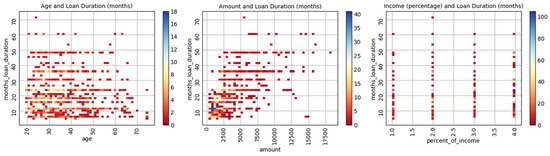
Figure 1.
Scatterplots for selected numeric features.
A deeper analysis of multicollinearity within the German Credit dataset (as shown in Table 4) reveals that the Variance Inflation Factor (VIF) values for all predictors fall well within acceptable thresholds, indicating that multicollinearity is not a concern and does not pose a risk to model reliability.
Table 4.
VIF—German Credit dataset.
The distribution of data can be considered partially normal or normal (right skewed) for only three predictors, as seen in Figure 2. The remaining numerical predictors are dichotomous in nature.

Figure 2.
Data distributions—German Credit dataset.
Although boosting algorithms are generally more robust to outliers, models such as Support Vector Machines (SVMs) and Feedforward Neural Networks (FNNs) are more sensitive to extreme values. Therefore, it is imperative to minimize the impact of outliers to maintain model stability and ensure reliable performance. In this study, preliminary diagnostic tests confirm that the German Credit dataset contains no missing values or significant outliers, thereby reducing the need for additional corrective measures during preprocessing.
3.4. Data Preprocessing
In the data preprocessing phase, the primary objective is to prepare the datasets in a way that enables models to leverage the underlying data structure effectively. This involves initial checks for outliers and missing values. Since both the German and Taiwan datasets are free from missing values, imputation techniques were excluded from the preprocessing pipelines.
To streamline and modularize data transformation, Scikit-learn’s ColumnTransformer is employed as the core functionality within the pipelines. The transformation process begins with scaling, including both standardization and normalization. This step is critical, particularly for models such as Support Vector Machines (SVMs) and Feedforward Neural Networks (FNNs), which are highly sensitive to feature scaling. In contrast, tree-based boosting algorithms—such as Gradient Boosting, XGBoost, and LightGBM—are generally more robust to unevenly scaled features. However, Gradient Boosting is more susceptible to the effects of unscaled features than XGBoost and LightGBM, which possess built-in mechanisms to mitigate scaling issues.
For instance, in Gradient Boosting, features with larger scales may dominate gradient updates, potentially skewing the model by overemphasizing these variables while neglecting more predictive but smaller-scale features. Furthermore, such large-scale features often produce greater reductions in the loss function, making them preferred candidates for tree splits. This imbalance can disrupt the regularization mechanism and slow down convergence.
Additionally, encoding categorical variables is an essential preprocessing step, particularly for the German Credit dataset, which includes a mix of numerical and categorical data. While LightGBM can automatically handle categorical features internally, all other models require explicit one-hot encoding to ensure categorical variables are properly utilized. The transformation process is followed by imbalanced data treatment using the SMOTE algorithm, as recommended by Alam et al. (2020), to address class distribution issues and enhance classification performance.
Subsequently, the pipeline performs dimensionality reduction—either using system defaults or a predefined number of features—to reduce model complexity and computational cost. In total, seven distinct permutations are constructed, each with its own corresponding pipeline. These pipelines maintain a consistent train–test split of 70:30, using stratified sampling to preserve the class distribution in both sets.
Each pipeline is designed to handle both numerical and categorical features, applying scaling and encoding as necessary. Only pipelines configured for dimensionality reduction include this additional step. Finally, all pipelines encompass the full machine learning workflow, including training, scoring, and performance evaluation, forming a complete end-to-end analytics process.
3.5. Model Construction and Evaluation
A total of seven algorithms are employed in the training and model-fitting stages of the analytics pipeline. These classifiers—Support Vector Machine (SVM), Gradient Boosting, XGBoost, LightGBM, Feedforward Neural Network (FNN), Long Short-Term Memory (LSTM), and 1D Convolutional Neural Network (1D-CNN)—are selected based on their unique characteristics and suitability for the given classification problem.
- Support Vector Machine (SVM)SVM is a distance-based algorithm known for its effectiveness in handling classification problems and its inherent robustness to overfitting, particularly in high-dimensional spaces. SVM can operate with different kernel functions: the linear kernel, which assumes a parametric linear relationship between input features and the target, and the Radial Basis Function (RBF) kernel, which captures non-linear boundaries. The decision boundary is formed by identifying a hyperplane that maximizes the margin between classes. However, SVM is sensitive to outliers with both linear and RBF kernels, as extreme values can shift the decision boundary. The two most critical hyperparameters for tuning SVM performance are the regularization parameter (C) and the kernel parameter (γ). Of these, C plays a key role in balancing model complexity and generalization. A low value of C allows for a wider margin but may increase classification errors, while a high value of C seeks to classify all training examples correctly, potentially leading to overfitting.
- Boosting-Based AlgorithmsThree tree-based boosting methods are incorporated: traditional Gradient Boosting, as well as its modern, optimized counterparts, XGBoost and LightGBM.
- ○
- Gradient Boosting serves as a baseline model, building weak learners sequentially to minimize the overall loss.
- ○
- XGBoost improves upon traditional Gradient Boosting by offering regularization, parallelization, and handling of missing values, which enhances speed and accuracy.
- ○
- LightGBM further optimizes performance through leaf-wise tree growth, and it natively supports categorical features, one-hot encoding, and efficient training on large, sparse datasets.
Unlike models such as SVM and FNN, boosting methods do not require features to be scaled or normally distributed. They are also relatively robust to outliers. Key hyperparameters to tune for these models include learning rate, number of estimators (trees), and maximum tree depth, which collectively influence training speed and prediction accuracy. - Feedforward Neural Network (FNN)FNN is a parametric model composed of layers of interconnected nodes, where the primary learnable parameters are weights and biases. Training involves the forward pass, where inputs are transformed through hidden layers using activation functions (typically ReLU), and the output layer produces classification probabilities. The loss function (e.g., Cross-Entropy for classification) quantifies prediction error, which is minimized through backpropagation and optimization algorithms like Stochastic Gradient Descent (SGD) or Adam.FNNs are most effective when trained on large datasets, as their predictive performance can deteriorate in low-data environments. Tuning FNN performance involves optimizing several hyperparameters:
- ○
- Number of hidden layers and neurons per layer;
- ○
- Learning rate;
- ○
- Choice of optimizer (e.g., SGD vs. Adam);
- ○
- Regularization techniques (e.g., dropout, L2);
- ○
- Batch size and number of epochs.
For instance, an excessively high learning rate may cause the model to overshoot the optimal weights, while a very low rate may result in slow convergence or getting stuck in local minima. The Adam optimizer often improves convergence speed and performance by dynamically adjusting the learning rate for each parameter.
The Feedforward Neural Network (FNN) used in this study is implemented using the tf.keras.Sequential API from TensorFlow, with the following architectural and training specifications:
- Input Layer: Configured to match the number of input features in the dataset.
- Hidden Layers: A single dense (fully connected) layer with 64 units, followed by:
- ○
- Batch Normalization to stabilize and accelerate training.
- ○
- ReLU activation function to introduce non-linearity.
- ○
- Dropout (rate = 0.5) to prevent overfitting, combined with L2 regularization (λ = 0.001) to penalize large weights.
- Output Layer: A dense layer with a sigmoid activation function, suitable for binary classification tasks.
- Optimizer: Stochastic Gradient Descent (SGD) with a learning rate of 0.001 and momentum of 0.9, promoting smoother convergence and mitigating oscillations.
- Loss Function: Binary Cross-Entropy, commonly used in binary classification to quantify the difference between predicted and actual labels.
- Evaluation Metric: Accuracy, which measures the proportion of correct predictions during training and evaluation.
- Training Configuration: The model is trained for 50 epochs using a batch size of 16.
- Validation Strategy: A 20% validation split is applied to the training data to monitor generalization performance and detect overfitting during training.
Table 5 summarizes the key characteristics of the various classifiers implemented in this study.
Table 5.
High-level characteristics of classifiers.
In this study, the primary evaluation metric is the Area Under the Receiver Operating Characteristic Curve (AUC-ROC). AUC-ROC is widely used to evaluate classification models as it reflects the model’s ability to rank predictions by analyzing the trade-off between the True-Positive Rate (Recall) and the False-Positive Rate (1: specificity). Unlike accuracy, AUC does not directly measure misclassification errors; instead, it assesses how well the model discriminates between classes across various threshold settings.
However, while AUC is a popular metric, it is not without limitations. As discussed by Lobo et al. (2008), AUC can be insensitive to class imbalance, potentially yielding high values even when a model performs poorly on the minority class. This can be misleading in highly imbalanced datasets, where AUC may fail to reflect the model’s actual precision or recall. Furthermore, AUC does not account for the cost of different types of errors and may be inappropriate for scenarios where specific decision thresholds or business rules are important. AUC is especially less informative when comparing models that prioritize precision over recall, or vice versa.
To complement AUC, this study includes additional performance metrics to offer a more comprehensive evaluation of model effectiveness. As noted by Han et al. (2022), relying solely on error rate—a common practice in earlier works such as Jain et al. (2000) and Nelson et al. (2003)—can be misleading, especially in the context of imbalanced datasets. This is particularly relevant to the Taiwan Credit Card dataset, which is skewed, with 77.88% of observations labelled as “non-risky” and only 22.12% as “risky.”
To address this, the following four metrics are also employed (see Table 6) to provide a multi-dimensional assessment of model performance:
Table 6.
Performance measurements.
- Accuracy: Measures the proportion of total correct predictions relative to all predictions.
- Precision: Assesses the proportion of true-positive predictions among all instances predicted as positive.
- Recall (Sensitivity): Measures the proportion of actual positive cases that are correctly identified by the model.
- F1 Score: Represents the harmonic mean of precision and recall, offering a balanced measure that is particularly valuable for imbalanced classification tasks.
- Together, these metrics ensure a robust evaluation framework that goes beyond AUC alone, accounting for the complexities of imbalanced data and diverse classification objectives.
Table 6 depicts the performance metrics used throughout the model comparisons.
All the scores used in this study are based on prediction results.
4. Results
The experimental results are presented in both tabular and graphical formats, supplemented by variable importance visualizations. These results compare the performance of two distinct datasets—the German Credit and Taiwan Credit Card datasets—across three variations of analytics pipelines. Due to the stochastic nature of several classifiers (particularly Neural Networks), slight variations in results were observed across different runs.
Included in the analysis are feature importance rankings generated from various algorithms, providing insight into the most influential predictors. The ROC-AUC curves illustrate model discrimination performance, where the grey dotted line represents the baseline of random guessing.
This study employs three pipeline variations, each designed to evaluate classifier performance under different preprocessing and optimization scenarios. These include the following:
- Permutation-1: With or without SMOTE; uses default hyperparameters and evaluates performance based on the full feature set.
- Permutation-2: With or without SMOTE; uses optimized hyperparameters with the full feature set.
- Permutation-3: With or without SMOTE; uses optimized hyperparameters with a reduced feature set, consisting of top-performing predictors.
Each pipeline includes the following preprocessing steps: data scaling, categorical encoding, and SMOTE treatment for class imbalance.
The results of these permutations are summarized as follows:
- Table 7 and Figure 3: Permutation-1 applied to the German Credit dataset, using default hyperparameters and all features.
Table 7. German Credit Card dataset—Permutation-1.
- Table 8, Figure 4 and Figure 6: Permutation-2 applied to the German Credit dataset, using optimized hyperparameters and all features.
Table 8. German Credit Card dataset—Permutation-2.
- Table 9, Figure 5 and Figure 7: Permutation-3 applied to the German Credit dataset, using optimized hyperparameters and reduced features.
Table 9. German Credit Card dataset—Permutation-3.
- Table 10, Figure 14 and Figure 15: Permutation-2 applied to the Taiwan Credit dataset, using optimized hyperparameters and all features.
Table 10. Taiwan Credit Card dataset—Permutation-1.
Figure 3.
ROC for default hyperparameters (full features)—German Credit dataset (Permutation-1).
Figure 3.
ROC for default hyperparameters (full features)—German Credit dataset (Permutation-1).
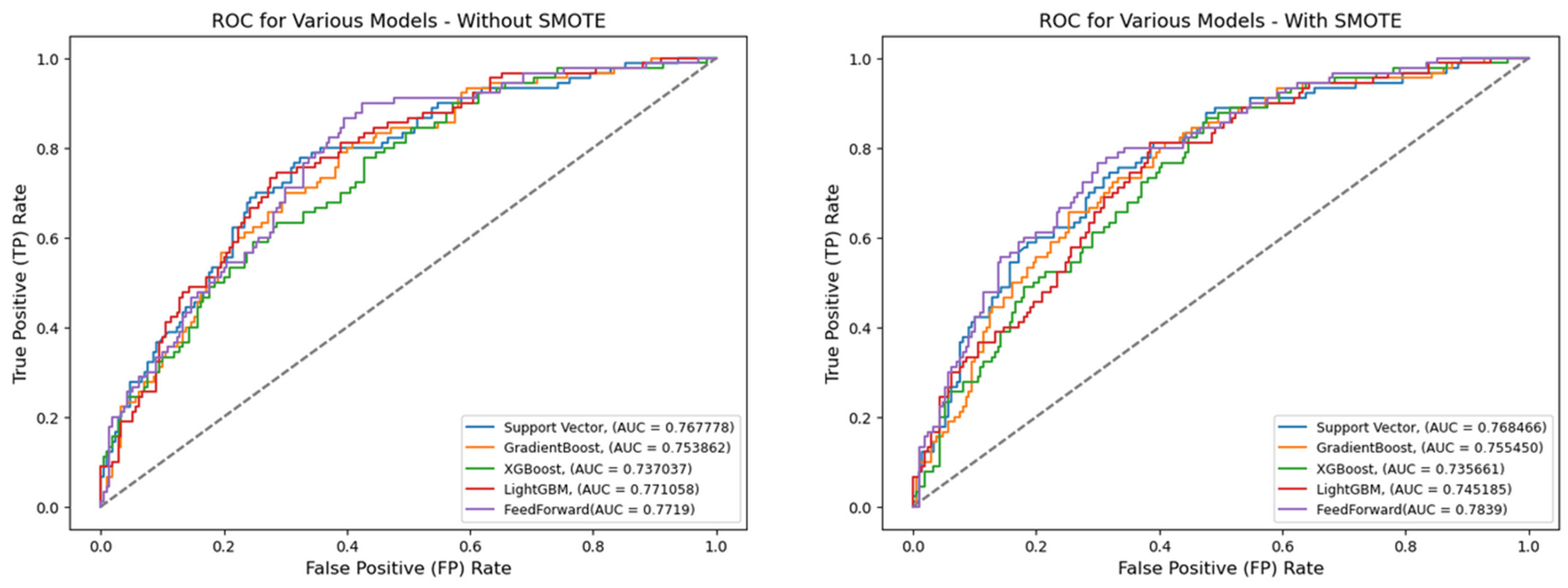
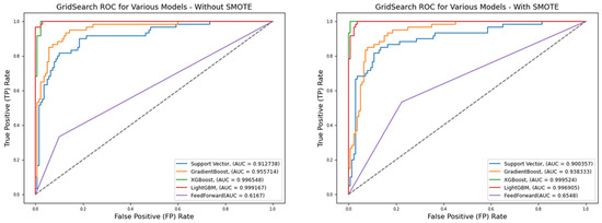
Figure 4.
ROC for best hyperparameters (full features)—German Credit dataset (Permutation-2).
Figure 4.
ROC for best hyperparameters (full features)—German Credit dataset (Permutation-2).
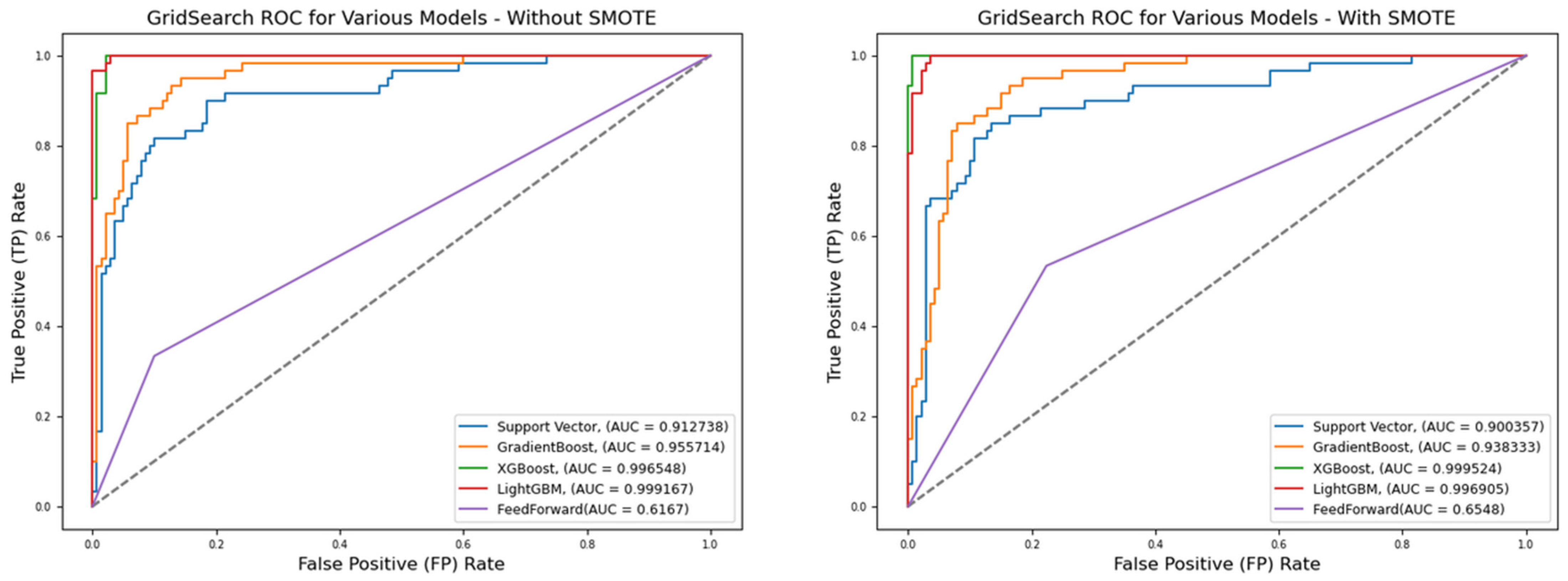
Figure 5.
ROC for best hyperparameters (reduced features)—German Credit dataset (Permutation-3).
Figure 5.
ROC for best hyperparameters (reduced features)—German Credit dataset (Permutation-3).
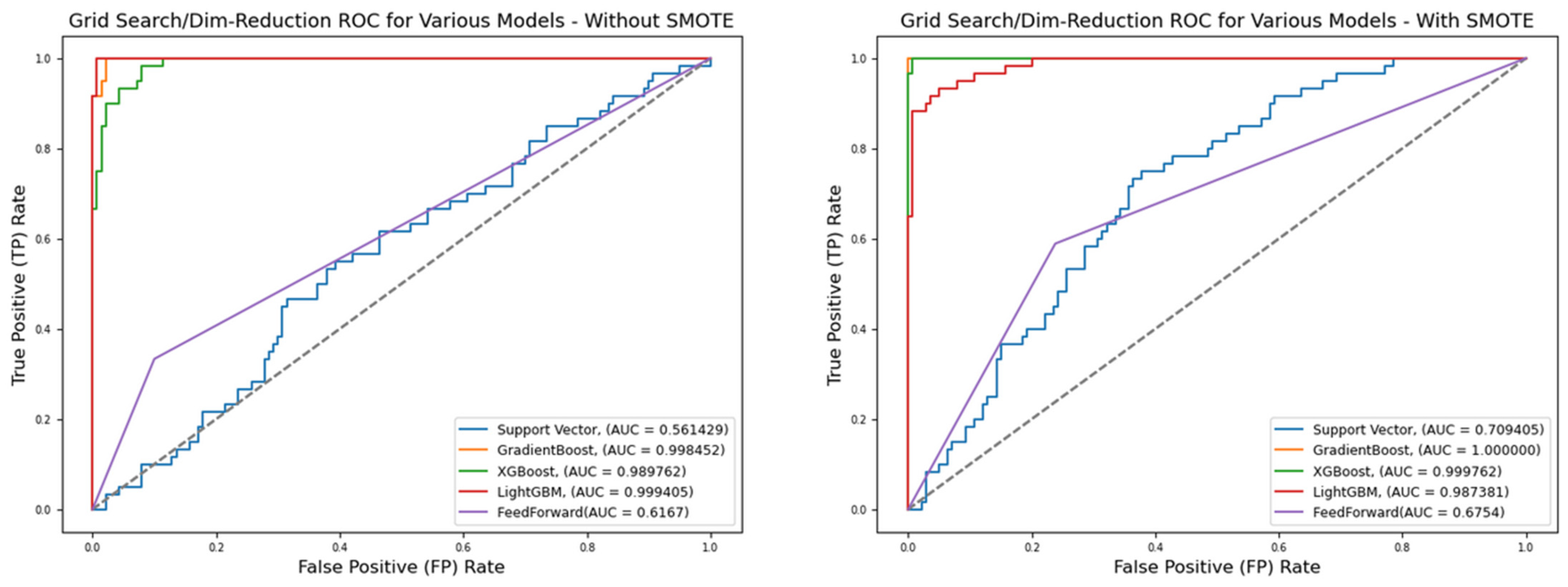

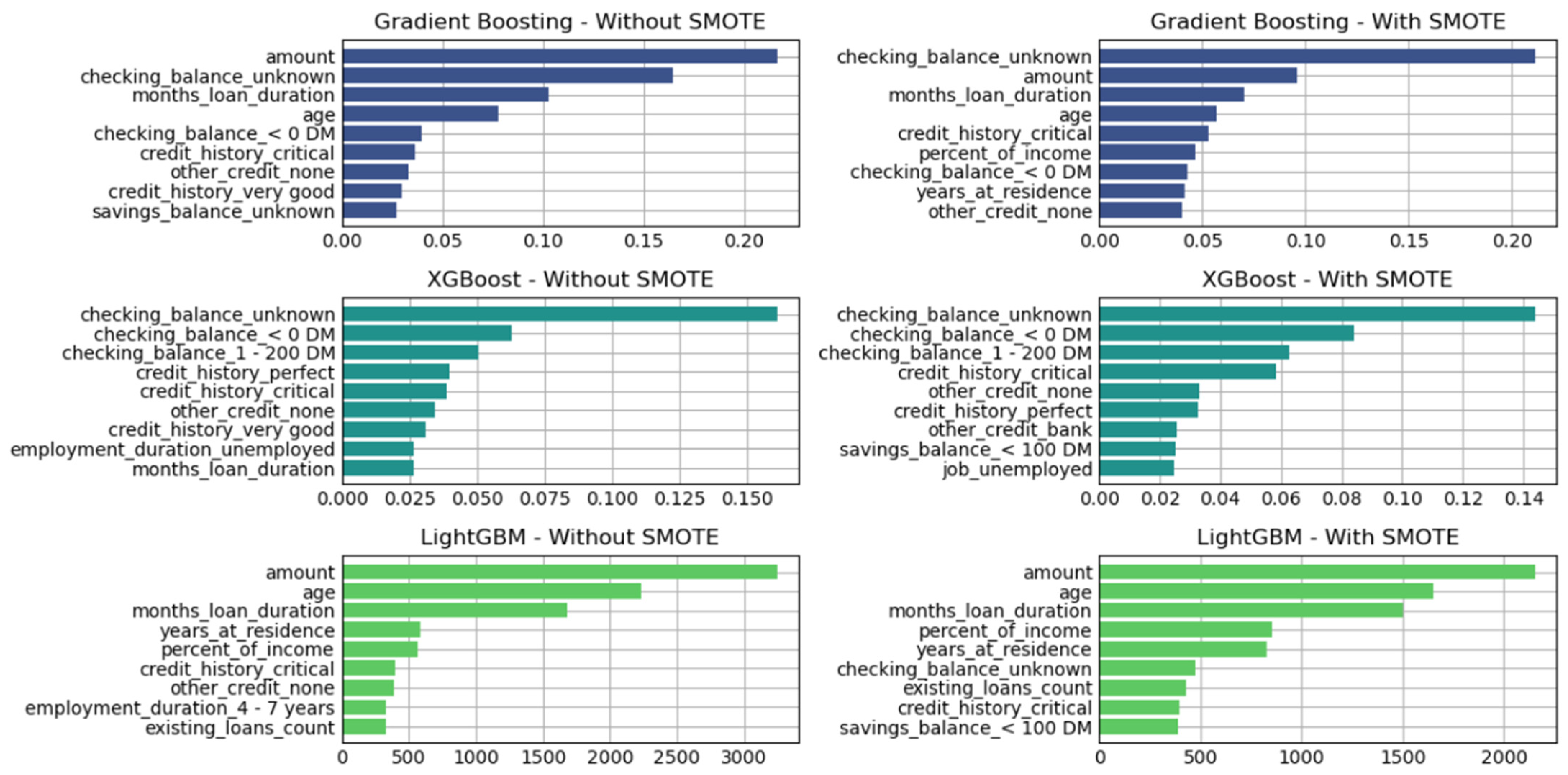
Figure 6.
Variable of importance for best hyperparameters (full features)—German Credit dataset (Permutation-2).
Figure 6.
Variable of importance for best hyperparameters (full features)—German Credit dataset (Permutation-2).
This structured approach allows for the systematic comparison of model performance under varying preprocessing conditions, classifier configurations, and dataset characteristics.
The optimal hyperparameters for each classifier, identified through grid search with and without SMOTE, are summarized as follows:
- Support Vector Machine (SVM):{‘C’: 1, ‘gamma’: 0.1, ‘kernel’: ‘poly’}
- Gradient Boosting:{‘learning_rate’: 0.1, ‘max_depth’: 5, ‘n_estimators’: 100}
- XGBoost:{‘colsample_bytree’: 0.6, ‘learning_rate’: 0.05, ‘max_depth’: 7, ‘n_estimators’: 100, ‘subsample’: 1.0}
- LightGBM:{‘learning_rate’: 0.01, ‘max_depth’: 10, ‘n_estimators’: 500, ‘num_leaves’: 31}
- Feedforward Neural Network (FNN):{‘dropout_rate’: 0.2, ‘learning_rate’: 0.001, ‘momentum’: 0.9}
Each of the three pipeline permutations is accompanied by graphical depictions of performance metrics across all classifiers. Additionally, Permutations-2 and -3 include feature importance analyses, identifying the most significant predictors for Decision Tree-based models such as Gradient Boosting, XGBoost, and LightGBM. The remaining classifiers, including SVM and FNN, produced comparable performance, though without native feature importance mechanisms.
As shown in Figure 7 and Figure 8, the three tree-based algorithms consistently highlight the same key predictive features across all permutations—whether using default hyperparameters, grid-searched hyperparameters, or reduced feature sets. Specifically, the features “amount”, “checking_balance”, “credit_history”, and “saving_balance” repeatedly emerge as the top contributors to model performance.
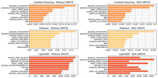
Figure 7.
Variable of importance for best hyperparameters (reduced features)—German Credit dataset (Permutation-3).
Figure 7.
Variable of importance for best hyperparameters (reduced features)—German Credit dataset (Permutation-3).

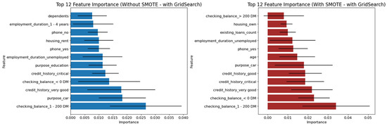
Figure 8.
Variable of importance for best hyperparameters (full features)—German Credit dataset (Permutation-2) with Feedforward Neural Network.
Figure 8.
Variable of importance for best hyperparameters (full features)—German Credit dataset (Permutation-2) with Feedforward Neural Network.

Similarly, Figure 9 and Figure 10 illustrate the Feedforward Neural Network’s variable importance, derived from permutation runs using both default and optimized hyperparameters. These results also reinforce the central role of “checking_balance” and “credit_history” as the two most influential features, mirroring the findings from the tree-based classifiers.
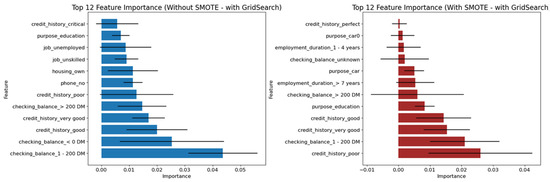
Figure 9.
Variable of importance for best hyperparameters (reduced features)—German Credit dataset (Permutation-3) with Feedforward Neural Network.
Figure 9.
Variable of importance for best hyperparameters (reduced features)—German Credit dataset (Permutation-3) with Feedforward Neural Network.

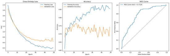
Figure 10.
Cross-Entropy (full features without SMOTE)—German Credit dataset (Permutation-1) with Feedforward Neural Network.
Figure 10.
Cross-Entropy (full features without SMOTE)—German Credit dataset (Permutation-1) with Feedforward Neural Network.
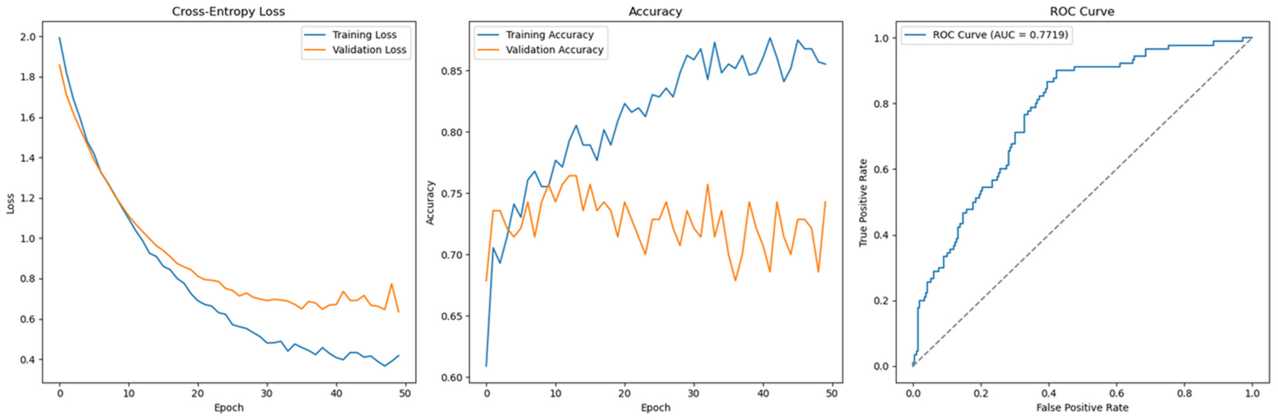
Figure 11, which presents the results of Permutation-1 without SMOTE, displays the Cross-Entropy loss curve for the feedforward model using the full feature set and default hyperparameters. The loss pattern suggests potential overfitting and a lack of convergence, indicating that the model may have struggled to generalize to unseen data. This behaviour is likely attributed to the class imbalance, which can hinder the model’s ability to learn meaningful patterns, especially in underrepresented classes.
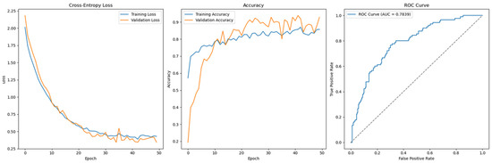
Figure 11.
Cross-Entropy (full features with SMOTE)—German Credit dataset (Permutation-1) with Feedforward Neural Network.
Figure 11.
Cross-Entropy (full features with SMOTE)—German Credit dataset (Permutation-1) with Feedforward Neural Network.
In contrast, Figure 12 shows the same feedforward model under Permutation-1 with SMOTE applied during preprocessing. The model demonstrates convergence and a stable decrease in Cross-Entropy loss, reflecting improved generalization and reduced overfitting. This highlights the effectiveness of SMOTE in addressing class imbalance, thereby enhancing the model’s learning stability and predictive performance.
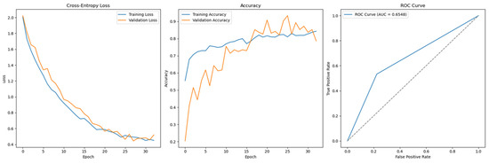
Figure 12.
Cross-Entropy (GridSearch full features without SMOTE)—German Credit dataset (Permutation-2) with Feedforward Neural Network.
Figure 12.
Cross-Entropy (GridSearch full features without SMOTE)—German Credit dataset (Permutation-2) with Feedforward Neural Network.
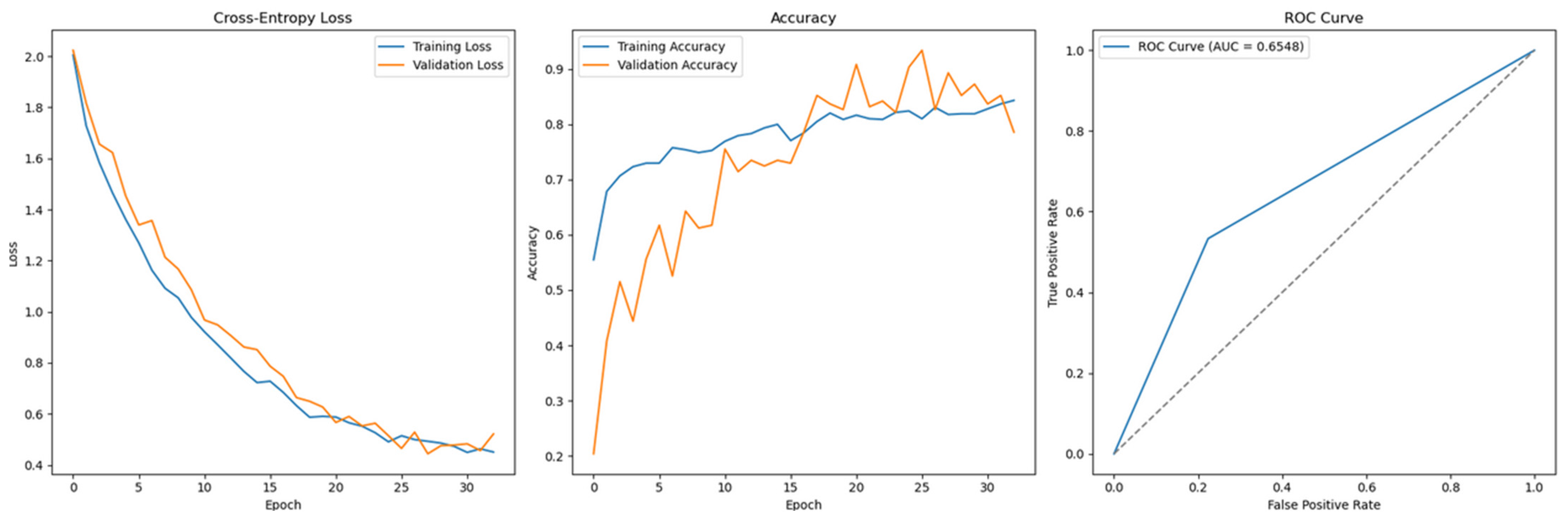
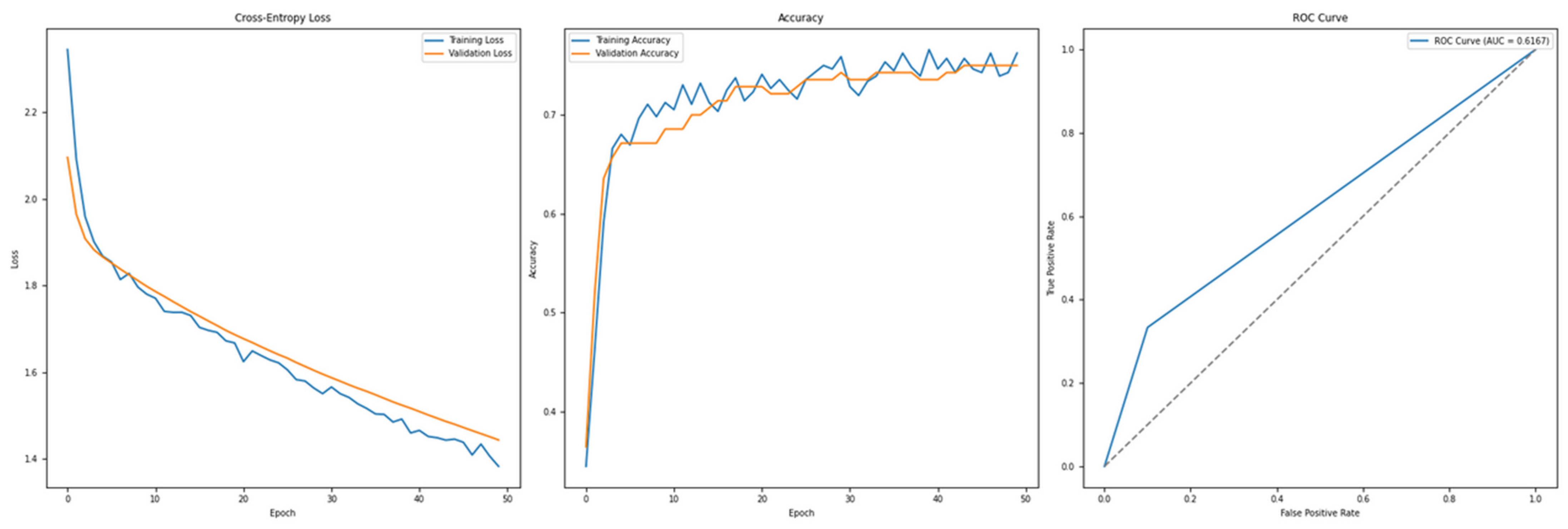
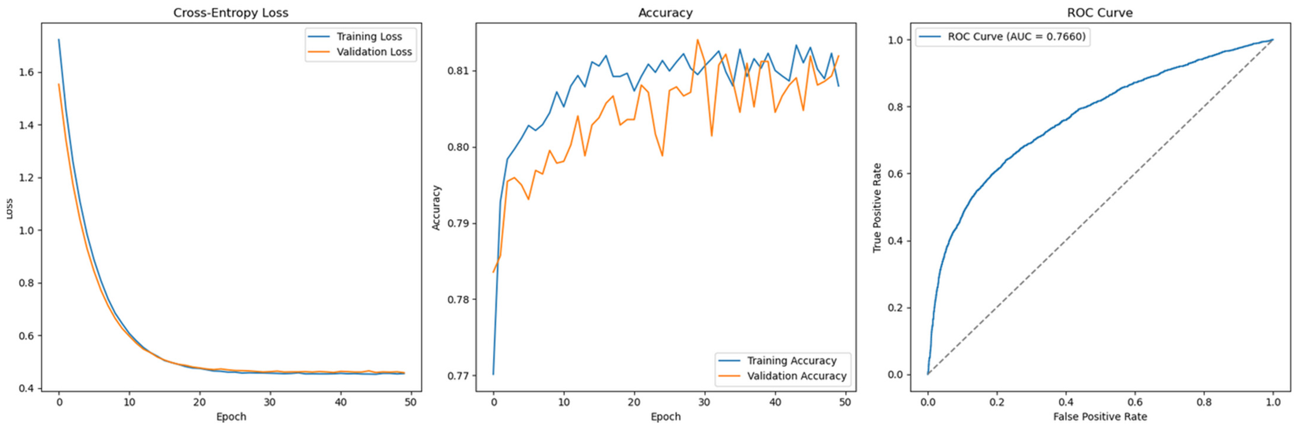
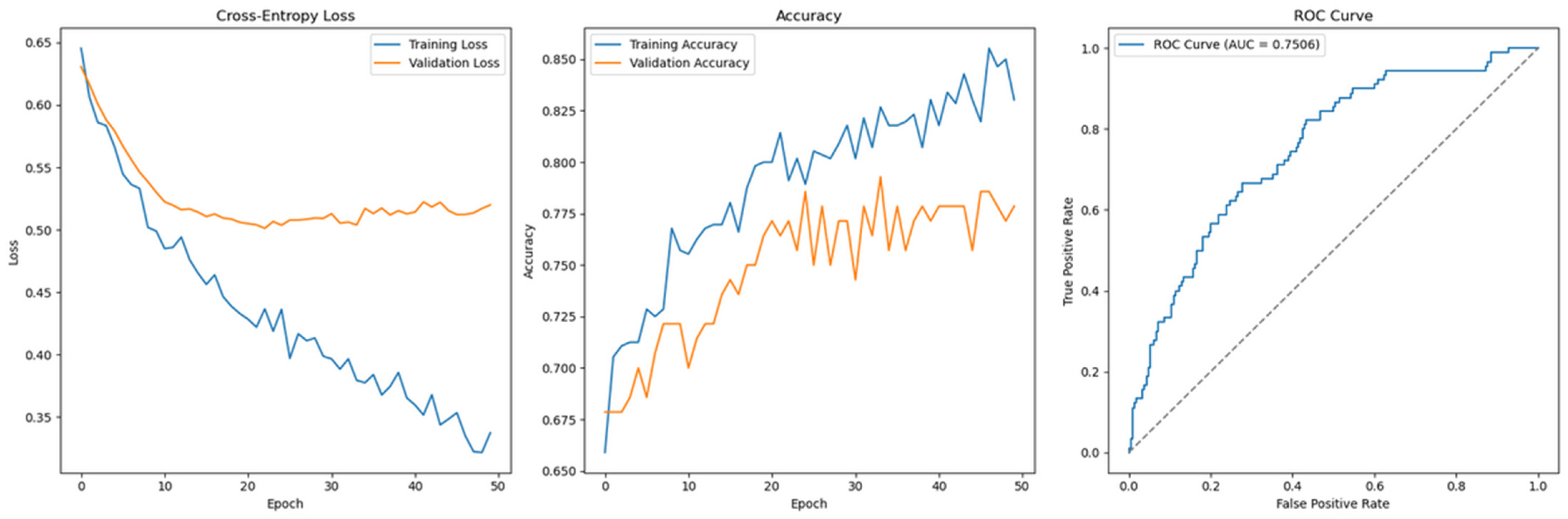
Figure 13, corresponding to Permutation-2 without SMOTE, illustrates the Cross-Entropy loss curve for the Feedforward Neural Network using the full feature set and grid-searched hyperparameters. The loss curve shows clear signs of convergence, and the accuracy plot indicates that validation accuracy closely tracks training accuracy throughout the training process. This alignment suggests that the model is generalizing well to unseen data, and the risk of overfitting is significantly reduced.
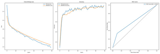
Figure 13.
Cross-Entropy (GridSearch full features with SMOTE)—German Credit dataset (Permutation-2) with Feedforward Neural Network.
Figure 13.
Cross-Entropy (GridSearch full features with SMOTE)—German Credit dataset (Permutation-2) with Feedforward Neural Network.
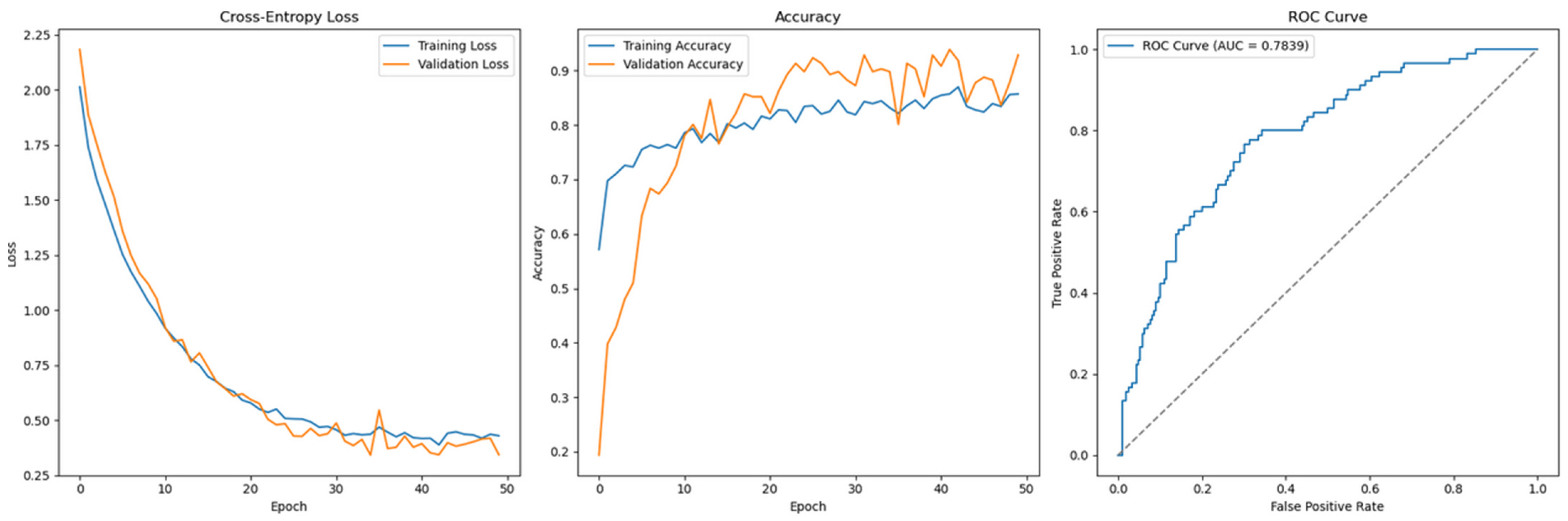
Similarly, Figure 14, which represents the same model configuration but with SMOTE applied, also demonstrates convergence and stable learning behaviour. The inclusion of SMOTE further enhances the model’s ability to generalize by addressing class imbalance. As with Figure 13, the model trained with SMOTE achieves strong generalization performance and avoids overfitting, reinforcing the importance of both hyperparameter optimization and class imbalance treatment in Neural Network training.
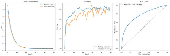
Figure 14.
Cross-Entropy (default hyperparameters, full features without SMOTE)—Taiwan Credit dataset (Permutation-1) with Feedforward Neural Network.
Figure 14.
Cross-Entropy (default hyperparameters, full features without SMOTE)—Taiwan Credit dataset (Permutation-1) with Feedforward Neural Network.
Finally, this study incorporates a control dataset from a Taiwanese credit card client, comprising 30,000 observations, which is significantly larger than the German Credit dataset. To maintain consistency and ensure comparability, the same Permutation-1 analytics pipeline, including all data transformation steps, is applied to this control dataset prior to model training. The Feedforward Neural Network architecture and configuration used here mirror those applied to the German dataset.
Table 10 presents the performance results. As expected, the larger dataset size enhances the predictive performance of the feedforward model, demonstrating improved accuracy and generalization. However, this improvement comes at the cost of increased training time, which is notably higher for the larger dataset.
Regarding classifier performance, Support Vector Machine, Gradient Boosting, XGBoost, and LightGBM all exhibit strong training and generalization capabilities using default hyperparameters, as reflected in Table 10. For the Feedforward Neural Network, Figure 15 shows a smooth convergence of the model trained with default hyperparameters, indicating good generalization.
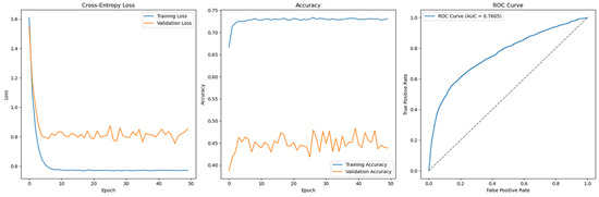
Figure 15.
Cross-Entropy (default hyperparameters, full features with SMOTE)—Taiwan Credit dataset (Permutation-1) with Feedforward Neural Network.
Figure 15.
Cross-Entropy (default hyperparameters, full features with SMOTE)—Taiwan Credit dataset (Permutation-1) with Feedforward Neural Network.
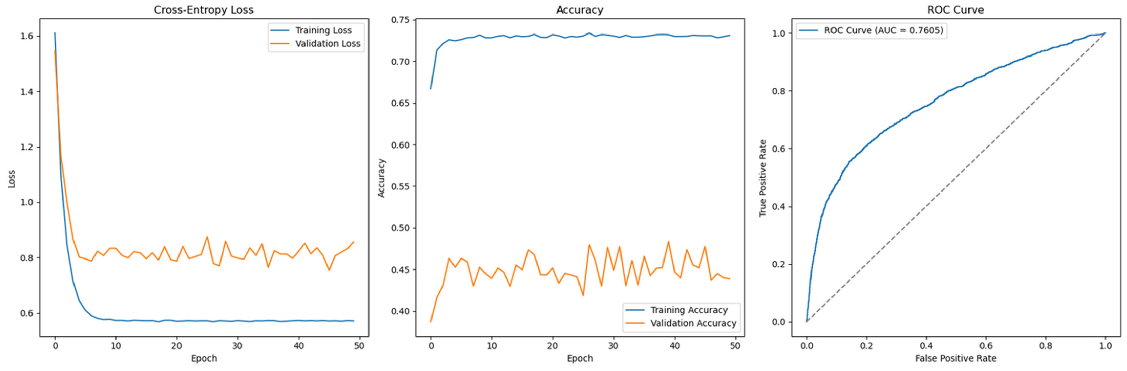
Interestingly, when SMOTE is applied to address class imbalance, the feedforward model exhibits non-convergent behaviour, as shown in Figure 16. Contrary to expectations, the model trained with SMOTE generalizes poorly, highlighting a counterintuitive result. This suggests that while SMOTE is generally beneficial in imbalanced scenarios, its effectiveness may vary depending on dataset characteristics, model architecture, and hyperparameter configurations.

Figure 16.
Cross-Entropy (default hyperparameters, full features with SMOTE)—German Credit dataset (Permutation-1) with LSTM.
Figure 16.
Cross-Entropy (default hyperparameters, full features with SMOTE)—German Credit dataset (Permutation-1) with LSTM.
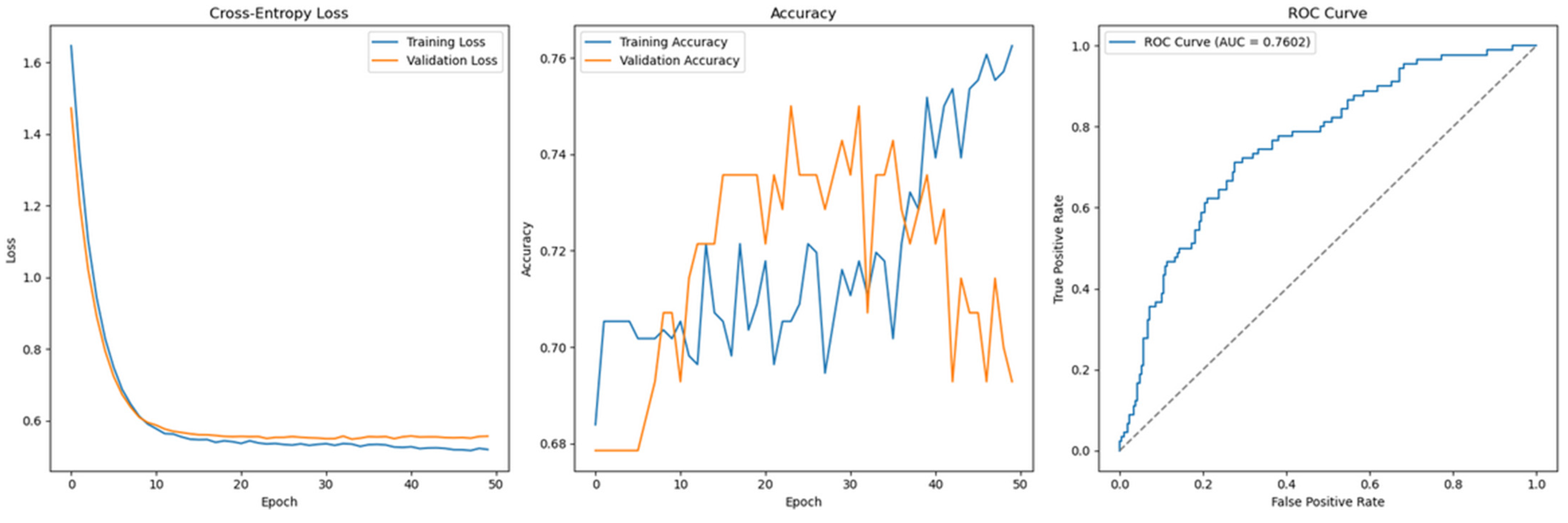
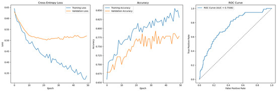
Figure 17.
Cross-Entropy (default hyperparameters, full features with SMOTE)—German Credit dataset (Permutation-1) with 1D-CNN.
Figure 17.
Cross-Entropy (default hyperparameters, full features with SMOTE)—German Credit dataset (Permutation-1) with 1D-CNN.
The final two configurations tested in this study are based on Long Short-Term Memory (LSTM) networks and 1D Convolutional Neural Networks (1D-CNNs). Given that both the German Credit and Taiwan Credit datasets are tabular in nature, only the German dataset is used for illustration purposes in this context.
- LSTM ConfigurationThe LSTM model is designed to handle sequential input data and includes the following components:
- ○
- Data Transformation: The dataset is reshaped to ensure that the number of features is divisible by the number of time steps, allowing for the proper formation of 3D input tensors required by LSTM models.
- ○
- LSTM Layer: The first layer consists of 64 units (neurons) with return_sequences = True, which outputs a sequence of hidden states across all time steps, maintaining the 3D tensor structure. L2 regularization is applied with a value of 0.01 to penalize large weights and reduce the risk of overfitting.
- ○
- Dropout Layer: A dropout rate of 0.3 is used to randomly deactivate 30% of the neurons during training, further mitigating overfitting.
- ○
- Output Layer: A sigmoid activation function is used to produce a binary classification output, indicating the likelihood of default.
- 1D-CNN ConfigurationThe 1D Convolutional Neural Network is structured to process tabular data treated as 1D sequences and consists of the following layers:
- ○
- First Convolutional Layer: Contains 64 filters with a kernel size of 3, using ReLU activation. This layer extracts 64 local features (feature maps) from the input.
- ○
- Max Pooling Layer: Uses a pool size of 2 to reduce the length of each feature map by half, thereby lowering dimensionality and retaining dominant features. This also helps reduce overfitting.
- ○
- Dropout Layer: A dropout rate of 0.3 is applied following the pooling layer to randomly deactivate 30% of the neurons during training.
- ○
- Second Convolutional Layer: Comprises 32 filters to extract deeper, more abstract patterns from the previously pooled feature maps.
- ○
- Global Average Pooling: This layer reduces each feature map to a single scalar value by averaging its values, reducing the output to a fixed-size vector and minimizing overfitting risk.
- ○
- Second Dropout Layer: An additional dropout rate of 0.2 is applied to further regularize the model by deactivating 20% of the neurons before final classification.
A comparative analysis of model performance between Table 7 (Permutation-1) and Table 8 (Permutation-2) clearly demonstrates that, with or without SMOTE treatment, pipelines consistently perform better when grid-searched hyperparameters are applied. For instance, under default hyperparameter settings, classifiers, such as Support Vector Machine, Gradient Boosting, XGBoost, and LightGBM, achieve accuracy scores ranging from 0.7133 to 0.7367 without SMOTE. With SMOTE treatment, these values decrease slightly to between 0.7000 and 0.7267. In terms of AUC, models without SMOTE range from 0.7370 to 0.7719, whereas SMOTE-treated models show marginal improvements, with AUCs between 0.7357 and 0.7685.
Interestingly, while the Feedforward Neural Network (FNN) performs comparably to other models under Permutation-1, Table 8 highlights a more significant performance gap when grid-searched hyperparameters are used. Under Permutation-2, the AUC scores for all models (excluding FNN) improve markedly, ranging from 0.8567 to 0.9867 without SMOTE and from 0.7033 to 0.9933 with SMOTE. A similar trend is observed in reduced feature scenarios, where AUC ranges from 0.9179 to 0.9993 (without SMOTE) and 0.9138 to 0.9999 (with SMOTE).
However, this performance improvement does not extend to the FNN, where SMOTE application results in deteriorating performance, with AUC dropping from 0.7300 to 0.6548. This outcome is counterintuitive, as all other algorithms either maintain or improve performance when SMOTE is applied.
Across all three permutations, it is evident that SMOTE fails to enhance FNN performance. Neither hyperparameter tuning nor dimensionality reduction improves its ability to generalize on imbalanced data. In Permutation-3, although Support Vector Machine shows some degradation in performance under reduced features, Gradient Boosting, XGBoost, and LightGBM maintain their robustness and strong predictive capacity.
Similar findings are reflected in the control dataset (Taiwan Credit), which has a larger number of observations. Table 10 shows that under Permutation-1 with default hyperparameters, all classifiers, including FNN, achieve comparable performance. Accuracy for models without SMOTE ranges from 0.8136 to 0.8208, while SMOTE-treated models range from 0.7802 to 0.8131. AUC values range from 0.7078 to 0.7825 (without SMOTE) and 0.7497 to 0.7714 (with SMOTE). Of note, the Support Vector Machine performs slightly worse with SMOTE, suggesting that not all algorithms benefit uniformly from synthetic oversampling.
The feedforward network, however, demonstrates a distinct behaviour. As seen in Figure 15, the model converges well under default hyperparameters without SMOTE—training and validation loss curves are closely aligned by epoch 10, indicating good generalization. In contrast, Figure 16 shows failure to converge when SMOTE is applied, with Cross-Entropy loss increasing and poor generalization emerging.
The model configuration for FNN includes the following:
- Input layer matching the number of features;
- Dense hidden layer with 64 neurons (initialized using He Uniform);
- ReLU activation, Batch Normalization, and dropout (rate = 0.5);
- Sigmoid activation in the output layer;
- L2 regularization (λ = 0.01);
- Training with SGD optimizer, momentum = 0.9, learning rate = 0.001, and 5-fold stratified cross-validation to preserve class balance.
Despite testing multiple hyperparameter combinations, FNN continues to exhibit overfitting when trained on SMOTE-augmented data. The issue arises because SMOTE-generated synthetic samples may not adequately represent the true distribution of the minority class, leading the model to overfit on synthetic patterns rather than learning generalizable features. With the minority class comprising only 20% of the dataset, SMOTE overcompensates, inflating the minority class and exacerbating the overfitting problem.
In the case of the LSTM model, applying this architecture to non-temporal tabular data introduces several limitations. LSTM networks are specifically designed to capture temporal dependencies, which are absent in tabular datasets like the German Credit data. Reshaping features into sequences to mimic time steps leads the LSTM to artificially learn dependencies between unrelated features, resulting in poor generalization or unnecessary model complexity. In such scenarios, non-sequential models like SVM, tree-based algorithms, or FNNs are more suitable.
Similarly, the 1D-CNN model assumes that neighbouring features exhibit meaningful sequential patterns—a condition often met in domains like signal or image processing but not in standard tabular data. Without natural feature ordering or sequential relationships, convolutional filters in 1D-CNNs fail to extract meaningful patterns, potentially learning artificial correlations that reduce performance. As a result, 1D-CNNs perform suboptimally when applied to tabular data lacking temporal or structured spatial characteristics.
5. Discussion
The following points summarize the main observations and provide possible explanations for the performance of the models evaluated in this study:
- Support Vector Machine (SVM) demonstrates consistent performance across most experimental configurations. However, a slight drop in accuracy is observed when SMOTE is applied to the larger Taiwan dataset. This may be attributed to the linear interpolation mechanism of SMOTE, which can generate synthetic minority class samples that overlap with the majority class, especially in high-dimensional spaces. As a distance-based model, SVM is sensitive to boundary distortions, and non-representative synthetic samples may compromise the decision margin, leading to degraded performance.
- The three tree-based ensemble algorithms—Gradient Boosting, XGBoost, and LightGBM—deliver the most consistent and superior performance overall. All experimental results confirm their robustness in binary classification tasks for tabular data. These algorithms outperform both SVM and Feedforward Neural Networks across several dimensions:
- ○
- Imbalance Handling: Even when the minority class is underrepresented, tree-based ensembles perform well, with or without SMOTE.
- ○
- Improved Accuracy: As ensemble methods, they reduce bias and variance by aggregating multiple base learners.
- ○
- Generalization Capability: Overfitting is less evident in these models, as validation on unseen data consistently yields high accuracy.
- ○
- Model Stability: Tree-based ensembles are resilient to outliers and noise, as they “average out” the effects of less reliable base models, leading to more stable predictions.
- The Feedforward Neural Network (FNN) underperforms in comparison to both SVM and the tree-based methods. Notably, FNN fails to converge when trained on SMOTE-treated datasets. The network tends to overfit synthetic samples, which are interpolated between real minority class instances. As demonstrated in Permutations-1 and -2, FNNs are particularly prone to overfitting on these artificially generated patterns. Moreover, once overfitting occurs, hyperparameter tuning becomes more difficult, further limiting performance improvements.
- LSTM and 1D-CNN architectures prove to be unsuitable for the datasets used in this study. Both the German Credit dataset and the Taiwan Credit dataset are tabular in nature and lack an inherent temporal structure. While attempts were made to reshape the data into time step sequences (e.g., simulating transactions over time), these transformations fail to introduce meaningful sequential patterns. As a result, both the LSTM and 1D-CNN models exhibit unstable generalization performance, particularly when evaluated on unseen data (as shown in Figure 17). These architectures are more appropriate for domains where sequential or spatial dependencies naturally exist.
- Finally, this study reinforces the importance of careful treatment of class imbalance during preprocessing. While SMOTE is a widely adopted oversampling technique, it does not universally improve performance. In this study, algorithms such as SVM, FNN, LSTM, and 1D-CNN show reduced generalization when trained on SMOTE-augmented data. This outcome underscores the need for the algorithm-specific evaluation of oversampling strategies and highlights the superior robustness of tree-based ensemble methods under class imbalance conditions.
6. Further Studies
While SMOTE was the primary oversampling technique explored in this study for addressing class imbalance, alternative resampling methods merit further investigation. As suggested by Alam et al. (2020), methods, such as Random Oversampling, ADASYN, k-means SMOTE, Borderline-SMOTE, and SMOTE-Tomek, offer distinct mechanisms for generating synthetic samples and may lead to more robust generalization. The poor performance observed with SMOTE in conjunction with Feedforward Neural Networks highlights the need for more nuanced oversampling strategies that avoid overfitting on synthetic data.
An alternative method introduced by Chen et al. (2018), the Synthetic Neighbourhood Generation (SNG) approach, shows promise by creating synthetic samples near the decision boundary of the minority class. Unlike traditional interpolation methods, SNG emphasizes generating higher-quality synthetic examples that enhance classifier learning without inducing bias or redundancy. Incorporating SNG or similar techniques in future studies may lead to better performance, particularly for classifiers like Neural Networks, which are sensitive to noisy or unrepresentative input patterns.
Beyond oversampling, further research should explore non-standardized preprocessing pipelines, as proposed by Zelaya (2019), which involve selectively including or excluding specific transformation steps (e.g., handling outliers, dealing with missing data, or applying normalization). This concept of pipeline volatility encourages adaptive strategies that tailor the preprocessing flow to the model and data characteristics, which could yield more consistent and interpretable results.
Given the superior performance of tree-based boosting algorithms (Gradient Boosting, XGBoost, and LightGBM), future research should investigate how these models perform under additional pipeline permutations, such as the following:
- Introducing clear outliers to evaluate robustness.
- Applying dimensionality reduction techniques such as Principal Component Analysis (PCA) and Recursive Feature Elimination (RFE).
- Utilizing built-in parameters like scale_pos_weight (available in XGBoost and LightGBM) to handle class imbalance more effectively.
Furthermore, in high-dimensional settings, enhancements such as adaptive feature selection and the use of custom loss functions that penalize noisy or redundant features may improve learning efficiency. For example, Grønlund et al. (2020) argue that the success of Gradient Boosting cannot be fully explained by margin size alone and propose considering base learner prediction strength as a more accurate explanatory factor. Combining boosting methods with other models—such as k-Nearest Neighbours (k-NN), Support Vector Machines (SVMs), or clustering-based approaches—may also offer gains through hybrid ensemble frameworks.
The results of this study indicate that the Feedforward Neural Network (FNN), while powerful in theory, underperformed compared to tree-based methods and SVMs, particularly when trained on SMOTE-treated data. Further investigation is warranted into the architectural design and optimization strategies of FNNs.
Key areas for future exploration include the following:
- Network depth and width: The number of layers (depth) and neurons per layer (width) can significantly impact model performance. Finding the optimal architecture for a given dataset requires both technical rigor and intuitive design.
- Regularization strategies: Methods such as dropout, L2 regularization, and Early Stopping play a vital role in reducing overfitting. A more exhaustive tuning of these techniques could improve generalization.
- Optimization techniques: This study primarily relied on SGD with momentum; however, further exploration of adaptive optimizers such as Adam and RMSprop, as well as learning rate schedules, may improve convergence and final performance.
- Advanced training techniques: Techniques like Batch Normalization (to stabilize and speed up training) and Gradient Clipping (to address vanishing/exploding gradients) were not fully explored and could further enhance model robustness.
Given the complexity of tuning deep learning models, future studies would benefit from systematic hyperparameter search strategies, such as Bayesian optimization or AutoML frameworks, to more efficiently explore the configuration space.
7. Conclusions
This study offers a comprehensive exploration of various classifiers, analyzing their unique characteristics and performance across different data preprocessing techniques, including data cleansing, feature and label encoding, feature importance analysis, dimensionality reduction, class imbalance handling, and cross-validation. It highlights how model performance is closely tied to the permutations of preprocessing steps, the complexity of the model, the size and structure of the dataset, and the presence of underlying patterns within the data.
Notably, the findings confirm the superiority of tree-based ensemble methods, specifically Gradient Boosting, XGBoost, and LightGBM, which consistently outperform other classifiers across all experimental configurations. In contrast, Support Vector Machines and Feedforward Neural Networks exhibit inconsistent performance, particularly when trained on data treated with SMOTE. These results underscore the fact that not all classifiers benefit equally from oversampling techniques and that model choice must be tailored to both data characteristics and preprocessing strategies.
Another key insight is the importance of hyperparameter tuning. This study clearly shows that reliance on default settings often leads to suboptimal outcomes, whereas grid search optimization significantly enhances model performance. While hyperparameter tuning is effective for SVM and tree-based models, it proves less feasible for Feedforward Neural Networks, primarily due to their tendency to overfit on synthetic samples and their sensitivity to class imbalance. This highlights the importance of computational resources and tuning strategies in the successful deployment of machine learning models in real-world applications such as credit risk assessment.
Furthermore, this study underscores that factors, such as data distribution, multicollinearity, class imbalance, and feature relevance, all play a significant role in shaping model performance, with different classifiers responding differently to these factors. This further reinforces the idea that model selection must be informed by a deep understanding of the dataset.
A final and critical conclusion concerns the importance of aligning model architecture with data structure. Attempts to impose artificial sequential structures in LSTM and 1D-CNN models—on tabular datasets lacking temporal dependencies—proved ineffective. These models failed to generalize, confirming that deep learning architectures must be applied where their assumptions (e.g., temporal or spatial continuity) are valid. As such, model selection must be grounded in domain knowledge and a careful assessment of the data’s intrinsic properties.
In summary, this study concludes that for tabular, imbalanced, and non-sequential credit data, models such as Support Vector Machines and especially tree-based boosting algorithms provide superior stability, scalability, and accuracy. Moving forward, practitioners and researchers must ensure they thoroughly understand the data and apply preprocessing and model selection techniques that align with both the statistical and structural nature of the dataset, to build models that are not only high-performing but also interpretable and robust.
Author Contributions
Conceptualization, A.W.T. and D.T.; methodology, A.W.T. and D.T.; software, A.W.T. and D.T.; validation, A.W.T. and D.T.; formal analysis, A.W.T. and D.T. All authors have read and agreed to the published version of the manuscript.
Funding
This research received no external funding.
Informed Consent Statement
Informed consent was obtained from all subjects involved in the study.
Data Availability Statement
Data are contained within the article.
Acknowledgments
Sincere thanks to Ong Seng Huat, UCSI, Malaysia, and Dat Tran, University of Canberra, for their constructive comments.
Conflicts of Interest
The authors declare no conflicts of interest.
References
- Abadi, M., Agarwal, A., Barham, P., Brevdo, E., Chen, Z., Citro, C., Corrado, G. S., Davis, A., Dean, J., & Devin, M. (2016). Tensorflow: Large-scale machine learning on heterogeneous distributed systems. arXiv, arXiv:1603.04467. [Google Scholar]
- Alam, T. M., Shaukat, K., Hameed, I. A., Luo, S., Sarwar, M. U., Shabbir, S., Li, J., & Khushi, M. (2020). An investigation of credit card default prediction in the imbalanced datasets. IEEE Access, 8, 201173–201198. [Google Scholar]
- Al-Bdour, G., Al-Qurran, R., Al-Ayyoub, M., & Shatnawi, A. (2019). A detailed comparative study of open source deep learning frameworks. arXiv, arXiv:1903.00102. [Google Scholar]
- Altman, E. I. (1968). Financial ratios, discriminant analysis and the prediction of corporate bankruptcy. The Journal of Finance, 23(4), 589–609. [Google Scholar] [CrossRef]
- Altman, E. I., Marco, G., & Varetto, F. (1994). Corporate distress diagnosis: Comparisons using linear discriminant analysis and neural networks (the Italian experience). Journal of Banking & Finance, 18(3), 505–529. [Google Scholar] [CrossRef]
- Beaver, W. H. (1966). Financial ratios as predictors of failure. Journal of Accounting Research, 4, 71–111. [Google Scholar] [CrossRef]
- Bell, T. B., Ribar, G. S., & Verichio, J. (1990). Neural nets versus logistic regression: A comparison of each model’s ability to predict commercial bank failures. Available online: https://egrove.olemiss.edu/cgi/viewcontent.cgi?article=1081&context=dl_proceedings (accessed on 25 October 2024).
- Black, F., & Scholes, M. (1973). The pricing of options and corporate liabilities. Journal of Political Economy, 81(3), 637–654. [Google Scholar] [CrossRef]
- Blum, M. (1974). Failing company discriminant analysis. Journal of Accounting Research, 12, 1–25. [Google Scholar] [CrossRef]
- Boritz, J. E., Kennedy, D. B., & Albuquerque, A. d. M. e. (1995). Predicting corporate failure using a neural network approach. Intelligent Systems in Accounting, Finance and Management, 4(2), 95–111. [Google Scholar] [CrossRef]
- Chen, Z., Lin, T., Xia, X., Xu, H., & Ding, S. (2018). A synthetic neighborhood generation based ensemble learning for the imbalanced data classification. Applied Intelligence, 48, 2441–2457. [Google Scholar] [CrossRef]
- Cheng, B., & Titterington, D. M. (1994). Neural networks: A review from a statistical perspective. Statistical Science, 9, 2–30. [Google Scholar]
- Ciampi, F., & Gordini, N. (2013). Small enterprise default prediction modeling through artificial neural networks: An empirical analysis of i talian small enterprises. Journal of Small Business Management, 51(1), 23–45. [Google Scholar] [CrossRef]
- Croux, C., Jagtiani, J., Korivi, T., & Vulanovic, M. (2020). Important factors determining Fintech loan default: Evidence from a lendingclub consumer platform. Journal of Economic Behavior & Organization, 173, 270–296. [Google Scholar] [CrossRef]
- Curram, S. P., & Mingers, J. (1994). Neural networks, decision tree induction and discriminant analysis: An empirical comparison. Journal of the Operational Research Society, 45(4), 440–450. [Google Scholar] [CrossRef]
- Deakin, E. B. (1972). A discriminant analysis of predictors of business failure. Journal of Accounting Research, 10, 167–179. [Google Scholar] [CrossRef]
- Dong, H., Liu, R., & Tham, A. W. (2024). Accuracy comparison between five machine learning algorithms for financial risk evaluation. Journal of Risk and Financial Management, 17(2), 50. [Google Scholar] [CrossRef]
- Dutta, S., Bose, P., Goyal, V., Bandyopadhyay, P., & Kumar, S. (2021). Applying convolutional-GRU for term deposit likelihood prediction. International Journal of Engineering and Management Research, 11, 265–272. [Google Scholar] [CrossRef]
- Edmister, R. O. (1972). An empirical test of financial ratio analysis for small business failure prediction. Journal of Financial and Quantitative Analysis, 7(2), 1477–1493. [Google Scholar] [CrossRef]
- Fletcher, D., & Goss, E. (1993). Forecasting with neural networks: An application using bankruptcy data. Information & Management, 24(3), 159–167. [Google Scholar]
- Gao, J., Sun, W., & Sui, X. (2021). Research on default prediction for credit card users based on XGBoost-LSTM model. Discrete Dynamics in Nature and Society, 2021(1), 5080472. [Google Scholar] [CrossRef]
- García, S., Luengo, J., & Herrera, F. (2016). Tutorial on practical tips of the most influential data preprocessing algorithms in data mining. Knowledge-Based Systems, 98, 1–29. [Google Scholar] [CrossRef]
- Grønlund, A., Kamma, L., & Green Larsen, K. (2020). Margins are insufficient for explaining gradient boosting. Advances in Neural Information Processing Systems, 33, 1902–1912. [Google Scholar]
- Han, J., Pei, J., & Tong, H. (2022). Data mining: Concepts and techniques. Morgan Kaufmann. [Google Scholar]
- Hart, A. (1992). Using neural networks for classification tasks–some experiments on datasets and practical advice. Journal of the Operational Research Society, 43(3), 215–226. [Google Scholar]
- Hasan, B. M. S., & Abdulazeez, A. M. (2021). A review of principal component analysis algorithm for dimensionality reduction. Journal of Soft Computing and Data Mining, 2(1), 20–30. [Google Scholar]
- Hofmann, H. (1994). Statlog (german credit data). UCI Machine Learning Repository. [Google Scholar]
- Jain, A. K., Duin, R. P. W., & Mao, J. (2000). Statistical pattern recognition: A review. IEEE Transactions on Pattern Analysis and Machine Intelligence, 22, 4–37. [Google Scholar]
- Jiang, Y. (2022). A primer on machine learning methods for credit rating modeling. In B. W. Sloboda (Ed.), Econometrics—Recent advances and applications. IntechOpen. [Google Scholar] [CrossRef]
- Jo, H., Han, I., & Lee, H. (1997). Bankruptcy prediction using case-based reasoning, neural networks, and discriminant analysis. Expert Systems with Applications, 13(2), 97–108. [Google Scholar] [CrossRef]
- Karels, G. V., & Prakash, A. J. (1987). Multivariate normality and forecasting of business bankruptcy. Journal of Business Finance & Accounting, 14(4), 573–593. [Google Scholar]
- Lacher, R. C., Coats, P. K., Sharma, S. C., & Fant, L. F. (1995). A neural network for classifying the financial health of a firm. European Journal of Operational Research, 85(1), 53–65. [Google Scholar] [CrossRef]
- Lai, L. (2020, August 21–23). Loan default prediction with machine learning techniques. 2020 International Conference on Computer Communication and Network Security (CCNS), Xi’an, China. [Google Scholar]
- Li, X., Long, X., Sun, G., Yang, G., & Li, H. (2018, October 8–12). Overdue prediction of bank loans based on LSTM-SVM. 2018 IEEE SmartWorld, Ubiquitous Intelligence & Computing, Advanced & Trusted Computing, Scalable Computing & Communications, Cloud & Big Data Computing, Internet of People and Smart City Innovation (SmartWorld/SCALCOM/UIC/ATC/CBDCom/IOP/SCI), Guangzhou, China. [Google Scholar]
- Liu, Y., & Feng, H. (2024). Hybrid 1DCNN-attention with enhanced data preprocessing for loan approval prediction. Journal of Computer and Communications, 12(8), 224–241. [Google Scholar] [CrossRef]
- Lobo, J. M., Jiménez-Valverde, A., & Real, R. (2008). AUC: A misleading measure of the performance of predictive distribution models. Global Ecology and Biogeography, 17, 145–151. [Google Scholar] [CrossRef]
- Martin, D. (1977). Early warning of bank failure: A logit regression approach. Journal of Banking & Finance, 1(3), 249–276. [Google Scholar]
- Nelson, B. J., Runger, G. C., & Si, J. (2003). An error rate comparison of classification methods with continuous explanatory variables. IIE Transactions, 35, 557–566. [Google Scholar] [CrossRef]
- Ohlson, J. A. (1980). Financial ratios and the probabilistic prediction of bankruptcy. Journal of Accounting Research, 18, 109–131. [Google Scholar] [CrossRef]
- Ripley, B. D. (1994). Neural networks and related methods for classification. Journal of the Royal Statistical Society: Series B (Methodological), 56(3), 409–437. [Google Scholar] [CrossRef]
- Roh, Y., Heo, G., & Whang, S. E. (2019). A survey on data collection for machine learning: A big data-ai integration perspective. IEEE Transactions on Knowledge and Data Engineering, 33(4), 1328–1347. [Google Scholar] [CrossRef]
- Salchenberger, L. M., Cinar, E. M., & Lash, N. A. (1992). Neural networks: A new tool for predicting thrift failures. Decision Sciences, 23(4), 899–916. [Google Scholar] [CrossRef]
- Sarle, W. S. (1994, April 10–13). Neural networks and statistical models. 19th Annual SAS Users Group International Conference, Dallas, TX, USA. [Google Scholar]
- Serengil, S. I., Imece, S., Tosun, U. G., Buyukbas, E. B., & Koroglu, B. (2021, September 15–17). A comparative study of machine learning approaches for non performing loan prediction. 2021 6th International Conference on Computer Science and Engineering (UBMK), Ankara, Turkey. [Google Scholar]
- Sharda, R., & Wilson, R. (1996). Neural network experiments in business-failure forecasting: Predictive performance measurement issues. International Journal of Computational Intelligence and Organizations, 1(2), 107–117. [Google Scholar]
- Tae, K. H., Roh, Y., Oh, Y. H., Kim, H., & Whang, S. E. (2019, June 30). Data cleaning for accurate, fair, and robust models: A big data-AI integration approach. 3rd International Workshop on Data Management for End-to-End Machine Learning, Amsterdam, The Netherlands. [Google Scholar]
- Tam, K. Y., & Kiang, M. (1990). Predicting bank failures: A neural network approach. Applied Artificial Intelligence an International Journal, 4(4), 265–282. [Google Scholar] [CrossRef]
- Wang, J. C., & Perkins, C. B. (2019). How magic a bullet is machine learning for credit analysis? An exploration with FinTech lending data. Federal Reserve Bank of Boston. [Google Scholar]
- Wibawa, A. P., Utama, A. B. P., Elmunsyah, H., Pujianto, U., Dwiyanto, F. A., & Hernandez, L. (2022). Time-series analysis with smoothed convolutional neural network. Journal of Big Data, 9(1), 44. [Google Scholar] [CrossRef]
- Wilson, R. L., & Sharda, R. (1994). Bankruptcy prediction using neural networks. Decision Support Systems, 11(5), 545–557. [Google Scholar] [CrossRef]
- Whang, S. E., Roh, Y., Song, H., & Lee, J.-G. (2023). Data collection and quality challenges in deep learning: A data-centric ai perspective. The VLDB Journal, 32(4), 791–813. [Google Scholar] [CrossRef]
- White, H. (1989). Learning in artificial neural networks: A statistical perspective. Neural Computation, 1(4), 425–464. [Google Scholar] [CrossRef]
- Yeh, I. C. (2016). Default of credit card clients. UCI Machine Learning Repository, 10, C55S3H. [Google Scholar] [CrossRef]
- Yeh, I. C., & Lien, C. H. (2009). The comparisons of data mining techniques for the predictive accuracy of probability of default of credit card clients. Expert Systems with Applications, 36, 2473–2480. [Google Scholar] [CrossRef]
- Yoon, Y., Swales, G., Jr., & Margavio, T. M. (1993). A comparison of discriminant analysis versus artificial neural networks. Journal of the Operational Research Society, 44(1), 51–60. [Google Scholar] [CrossRef]
- Zelaya, C. V. G. (2019, April 8–11). Towards explaining the effects of data preprocessing on machine learning. 2019 IEEE 35th International Conference on Data Engineering (ICDE), Macao, China. [Google Scholar]
- Zhang, G., Hu, M. Y., Patuwo, B. E., & Indro, D. C. (1999). Artificial neural networks in bankruptcy prediction: General framework and cross-validation analysis. European Journal of Operational Research, 116(1), 16–32. [Google Scholar] [CrossRef]
- Zhao, W., Bhushan, A., Santamaria, A. D., Simon, M. G., & Davis, C. E. (2008). Machine learning: A crucial tool for sensor design. Algorithms, 1(2), 130–152. [Google Scholar] [CrossRef]
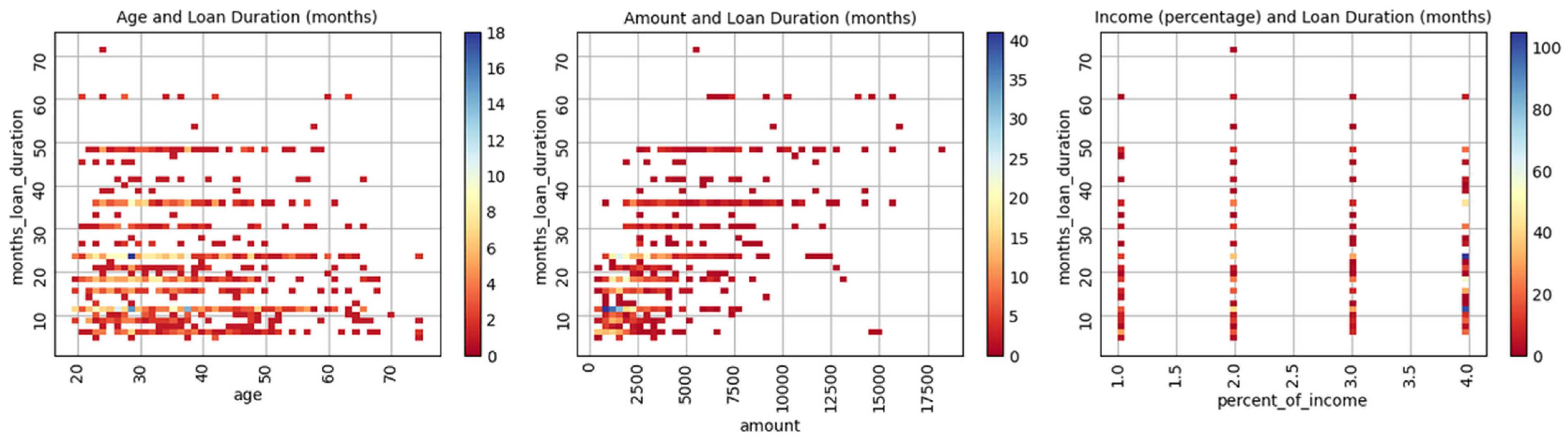
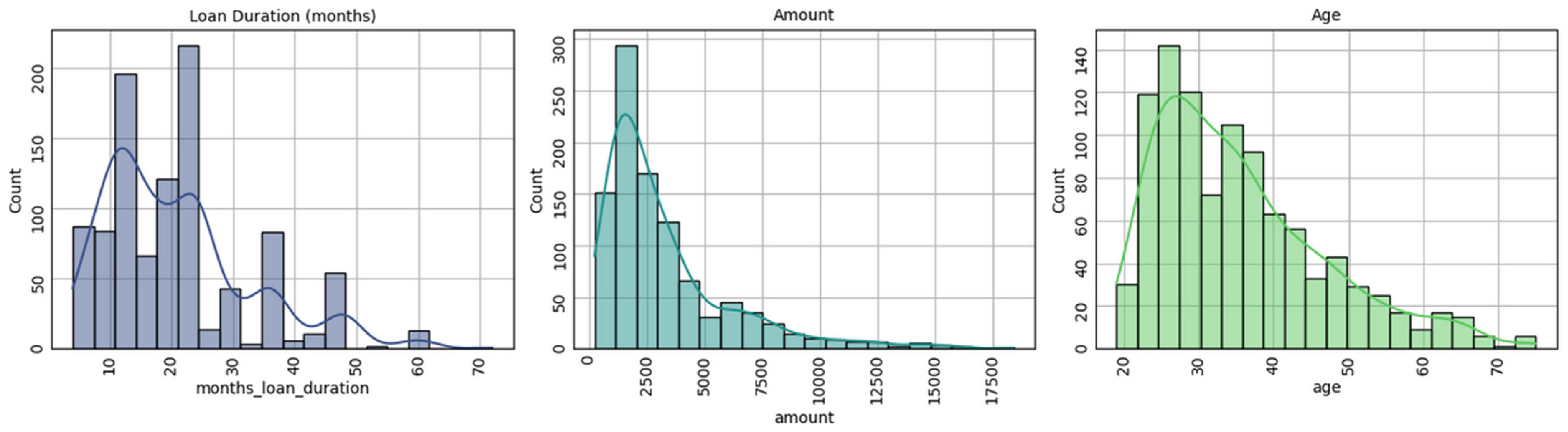
Disclaimer/Publisher’s Note: The statements, opinions and data contained in all publications are solely those of the individual author(s) and contributor(s) and not of MDPI and/or the editor(s). MDPI and/or the editor(s) disclaim responsibility for any injury to people or property resulting from any ideas, methods, instructions or products referred to in the content. |
© 2025 by the authors. Licensee MDPI, Basel, Switzerland. This article is an open access article distributed under the terms and conditions of the Creative Commons Attribution (CC BY) license (https://creativecommons.org/licenses/by/4.0/).