Determining the Flexible Ramping Capacity of Electric Vehicles to Enhance Locational Flexibility

Abstract

A high penetration level of renewable energy in a power system increases variability and uncertainty, which can lead to ramping capability shortage. This makes the stable operation of a power system difficult. However, appropriate management of electric vehicles (EVs) can overcome such difficulties. In this study, EVs were applied as a flexible ramping product (FRP), and a method was developed to increase the system ramping capability. When increasing the FRP to the amount required for the system, the effect on transmission lines cannot be neglected. Thus, the required FRP considering transmission constraints is calculated separately for each zone to secure deliverability. To make adjustment possible, the zonal available capacity is calculated by considering the probabilities of the location and the plugged and charged states of EVs. The applicability of EVs as an FRP resource is examined, and the results showed that they can be used at a more significant level considering the transmission constraints.

1. Introduction

Researchers have long pointed out the problems with power system operation due to increased renewable energy use. Previous studies have examined the impact of increased renewable energy use on power systems from diverse perspectives [1,2]. Controlling the output of renewable energy is not easy, and the controllable range is not broad, even if available. Therefore, power systems experience variability in the power output of renewable energy resources [3,4,5,6]. The predicted output of renewable resources has higher uncertainty than that of a conventional power generator; this intensifies the operational challenges of a power system. Therefore, flexibility must be ensured during the planning and operation of a power system so that it can respond to these risky conditions [7,8]. Otherwise, events with insufficient ramping capacity of generation would occur frequently [9]. This could lead to undesired outcomes such as wind curtailment [10]. This risk can reportedly be alleviated using a flexible ramping product (FRP) [11,12]. An FRP is extremely necessary for enhanced system flexibility and operational efficiency, particularly for systems with a significant proportion of power generated from renewable resources [13,14].

The Midcontinent Independent System Operator (MISO) and California Independent System Operator (CAISO) have established and have been managing a ramp market where FRPs are procured to prepare for the variability and uncertainty in the net load [15,16,17]. However, meeting the FRP requirements of a power system using only conventional generators has limitations. Research has been conducted on securing FRPs with alternative resources. Chen et al. [18] and Cui et al. [19] suggested methods of procuring FRPs through wind power, and Zhang and Kezunovic [20] performed early research on utilizing electric vehicles (EVs) as FRPs.

The persistent increase in the popularity of EVs is expected to contribute to environmental friendliness through de-carbonization in the transportation sector and enable EVs to serve as a resource for providing system flexibility through their charging and discharging interactions with power systems. The penetration level of renewable energy can be increased when higher system flexibility is ensured through EVs [21]. Vehicle-to-grid may serve as a storage resource for handling the intermittency of renewable energy output [22]. Existing research from this perspective has mostly applied EVs for frequency regulation [23] or providing reserve resources [24,25]. An EV owner can obtain a significant revenue as a reward for providing regulation reserves to a system operator [26]. However, such services require frequent charging and discharging cycles for a short time, which may affect the usability of EVs. In contrast, the required charging cycle of EVs for providing FRPs is typically 5–10 min with considerably less frequent utilization than that for the abovementioned services. Thus, applying EVs as an FRP resource is a more efficient approach.

Another advantage of applying EVs is that they are relatively unconstrained by the transmission congestion problem, which can occur in transmission lines connecting different zones. Large-scale conventional generators and renewable generators are typically far from regions with high power demand. Thus, the generated power is transmitted through several transmission lines to demand sites, and this condition is generally considered to be responsible for the transmission congestion problem. In contrast, utilizing EVs does not aggravate transmission congestion because they are typically distributed within regions with high load demand. Moreover, the mobility of EVs can enhance system conditions from the perspective of mitigating transmission congestion and reducing grid operation costs [27,28]. Adequate utilization of mobility can reduce curtailment for the energy capacity of renewable power; this can increase the integration of renewable energy [29]. Therefore, applying EVs as an FRP resource is more advantageous compared to using a conventional generator when transmission constraints are considered.

Existing research has considered the transmission congestion problem within the process of energy and ancillary service co-optimization [30,31]. However, research on transmission congestion that considers FRPs is insufficient. This paper examines the effects of FRPs on transmission constraints and the applicability of EVs as an FRP resource.

A method of securing FRPs by zone is proposed to consider transmission constraints. In addition, this paper describes a methodology of stochastically estimating the optimal location and the plugged and charged states of EVs to utilize them most efficiently and suggests an application of the method for system operation. Finally, the paper proposes a method of optimizing the operation of a power system with energy and FRPs using a conventional generator and EVs considering the charging and discharging characteristics of EVs.

The remainder of this paper is organized as follows: Section 2 describes the methodology of utilizing EVs as an FRP. The mathematical formulation is shown in Section 3. Case studies are presented in Section 4. To concentrate on the effect of applying FRP resources, a simulation was conducted excluding reserve products. Finally, Section 5 concludes the paper and proposes future research topics.

2. Methodology

2.1. Flexible Ramping Product

Power system load fluctuates constantly, and appropriate countering is essential for stable operation. Thus, operational flexibility is an important factor that must be secured. When the level of renewable energy penetration in a power system is considerably increased, the net load becomes more concentrated. The net load refers to the value of non-controllable generation such as renewable energy that is excluded from the normal load; it is characterized by variability and uncertainty. Variability is the change in the net load over time. In a state where the normal load does not change significantly, the variability in the net load increases with the penetration level of renewable energy. Uncertainty occurs because the variation of the net load cannot be precisely forecasted; it is produced by system contingencies or generator outage. Moreover, it increases with the penetration level of renewable energy. There is a limit to preventing the increase in variability and uncertainty using only the ramp rate of existing conventional generators. Thus, an FRP is required to ensure the operational flexibility of a power system.

An FRP is composed of flexible ramping up (FRU) and flexible ramping down (FRD) to compensate the upward and downward variations in the net load, respectively. The required capacities for FRU and FRD can be calculated as follows [32]:

$$FR{U}_{system,t}=\max \left\{\left[NetLoa{d}_{t+s}-NetLoa{d}_t\right]+Uncertaint{y}_{up,t+s},0\right\}$$

(1)

$$FR{D}_{system,t}=\max \left\{\left[NetLoa{d}_t-NetLoa{d}_{t+s}\right]+Uncertaint{y}_{down,t+s},0\right\}$$

(2)

where NetLoad_t+s − NetLoad_t and NetLoad_t − NetLoad_t+s refer to the variability in the net load. The FRP required at t + s is ensured at t, which captures the variability and uncertainty in the net load. Operational flexibility can be increased by procuring an FRP. FRP requirements are determined by zones for increased reliability. Such a method has been developed by the MISO and is applied below:

$${\displaystyle \sum _{z}FR{U}_{z,t}}\ge FR{U}_{system,t}$$

(3)

$${\displaystyle \sum _{z}FR{D}_{z,t}}\ge FR{D}_{system,t}$$

(4)

2.2. EV Utilization for FRP

An EV operates by charging and using a battery. Thus, connection with a power system is essential. An EV plugged in a system is equivalent to a battery with remarkable ramping capability, and it can be applied to the system for charging and discharging. Sufficient capacity can be secured through EVs because their use is expected to continue to increase [33]. Thus, EVs are appropriate as an FRP. To utilize EVs as an FRP, their location and plugged and charged states must be estimated. A probabilistic approach is proposed to calculate the applicable energy capacity of EVs at a specific time.

2.2.1. EV State Estimation

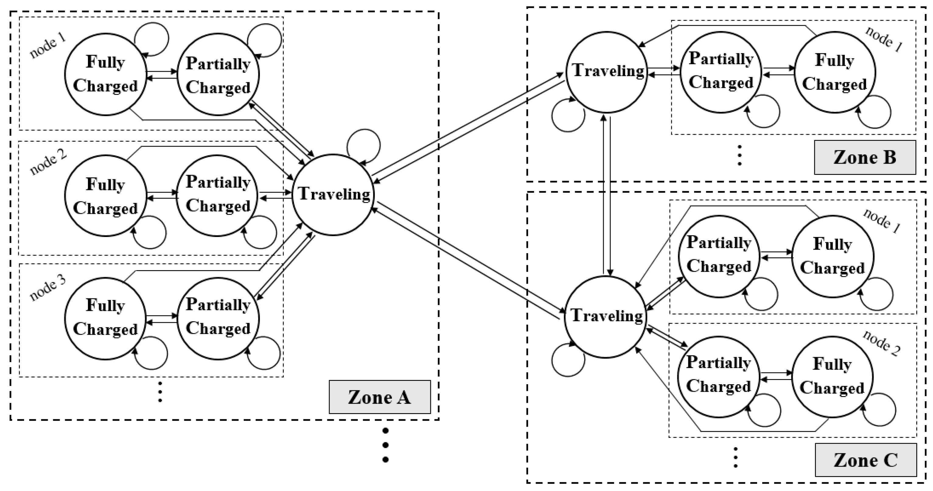
To utilize EVs as an FRP resource, it is necessary to predict the location and plugged and charged states. In this study, we calculated the usable capacity of an EV that changes over the interval time of a dispatch through stochastic estimation of EV states. The available capacity of an EV can be utilized for charging and discharging from a system and as an FRP resource. This process is presented as follows: The state of an EV is memoryless; it is determined only by the state of the immediately preceding time interval and is completely independent from past states. In addition, the EV state changes with time. The Markov chain is regarded as suitable for reflecting this property and can be used to model state transitions. Therefore, the Markov chain is applied to consider such states, as shown in Figure 1.

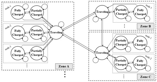
Figure 1. Markov chain for electric vehicle (EV) state estimation.

Figure 1 illustrates every state of an EV in a power system using the Markov chain. The power system consists of three zones and six nodes. First, the states of an EV can be classified as “traveling” and “plugged”. The EVs in the plugged state can be divided into those in the “fully charged” state and “partially charged” state. Every state can either be returned to its previous state or be transited to another state following the transition probability.

The change in each state complies with the following rules: if a traveling EV in one zone moves to another zone and parks there, it must pass through the traveling state in that zone. For example, a driver traveling with his EV in Zone A can park his car at a node in Zone C only after the EV passes through the traveling state in Zone C at least once. Additionally, the EV should pass through the traveling state of the zone every time it moves to other plugging nodes placed within the same zone. Note that the EV cannot transit from the traveling state to the fully charged state because it uses battery power while traveling. On the contrary, EVs in the fully charged and partially charged states can transit directly to the traveling state. A partially charged EV can transit to the following three types of states: remain unchanged, transit to the traveling state, or transit to the fully charged state. In the first type, the EV can provide its power to the grid from the partially charged state. The EV remains in this state until charging is complete. In the second type, the partially charged EV starts to drive. In the last type, the EV transits to the fully charged state when charging is completed. If an EV in this state is discharged, it changes to the partially charged state. Otherwise, it can remain fully charged or transit to the traveling state.

The location state indicates which zone an EV resides in. The probability of the number of EVs in each zone is assumed to follow a normal distribution with mean m_z and standard deviation σ_z [34]:

$$E_z~N\left(m_z,{\sigma }_z^2\right)=\frac{1}{\sqrt{2\pi }{\sigma }_z}{e}^{-\frac{{(k-m_z)}^2}{2{\sigma }^2}}$$

(5)

When a considerable number of vehicles exist, the probability of the number of vehicles traveling on a road follows the Poisson distribution [35]. The probability that a given number, k, of vehicles are traveling on a road is given by:

$$P_{tr}\left(k\right)=\frac{{\rho }^k}{k!}{e}^{-\rho }$$

(6)

where ρ is the population parameter value of the Poisson distribution. The term ρ refers to the average number of traveling EVs, which is calculated by dividing the arrival rate of vehicles into the traffic system by the reciprocal of the mean travel time. Therefore, (6) represents the probability that k EVs are traveling when the average number of traveling EVs is ρ. For example, if the average number of traveling vehicles is 100, then the probability that 90 vehicles are traveling is $P_{tr}\left(90\right)=\frac{{100}^{90}}{90!}{e}^{-100}\approx 0.025$. The probability that j EVs are parked out of ν EVs is represented by:

$$P_{pa}\left(j\right)={\displaystyle \underset{-\infty }{\overset{\infty }{\int }}\frac{{\rho }^{\left(v-j\right)}}{\left(v-j\right)!}{e}^{-\rho }\cdot \frac{1}{\sqrt{2\pi }{\sigma }_z}}{e}^{-\frac{{\left(v-m_z\right)}^2}{2{\sigma }_z^2}}dv$$

(7)

In this case, ν − j EVs would be traveling. The probability of this condition is derived using (6). Equation (7) can be obtained by combining the above two equations.

Because a system operator can utilize only parked EVs, the applicable capacity of EVs is calculated using the number of parked EVs. The applicable EV energy capacity differs according to the charged state of a parked EV. The charged state is divided into the partially charged state (pc) and fully charged state(fc). The energy distribution probabilities according to each state are given by:

$$E_{pc}~N\left(m_{pc},{\sigma }_{pc}^2\right)$$

(8)

$$E_{fc}~N\left(m_{fc},{\sigma }_{fc}^2\right)$$

(9)

The distribution of charged energy for the EVs is assumed to follow a normal distribution. With this distribution, the mean value of the fully charged state (m_fc) is the same as the chargeable maximum capacity of an EV battery with a standard deviation (σ_fc) of close to zero. The plugged EV energy distribution (P_pl) is calculated by combining the probabilities of the partially charged state (P_pc) and fully charged state (P_fc) and the charged energy distribution of each state in (8) and (9). This is formulated as follows:

$$E_{pl}~N\left(m_{pl},{\sigma }_{pl}^2\right)$$

(10)

$$m_{pl}=\frac{P_{pc}}{P_{pc}+P_{fc}}\cdot m_{pc}+\frac{P_{fc}}{P_{pc}+P_{fc}}\cdot m_{fc}$$

(11)

$${\sigma }_{pl}^2={\left(\frac{P_{pc}}{P_{pc}+P_{fc}}\right)}^2\cdot {\sigma }_{pc}^2+{\left(\frac{P_{fc}}{P_{pc}+P_{fc}}\right)}^2\cdot {\sigma }_{fc}^2$$

(12)

2.2.2. EV Available Energy and Power Estimation

The energy gained through the EVs in the system is estimated as follows: First, the cumulative energy distribution function of the plugged EV fleet is calculated by combining the parked probability of j EVs out of ν EVs with the distribution probability of energy:

$$\begin{array}{l}{K}_E(g)={\displaystyle \underset{-\infty }{\overset{g}{\int }}{\displaystyle \sum _{j=1}\left({\displaystyle \underset{-\infty }{\overset{\infty }{\int }}\frac{{\rho }^{\left(v-j\right)}}{\left(v-j\right)!}}\cdot e^{-\rho }\cdot \frac{1}{\sqrt{2\pi }{\sigma }_z}\cdot e^{-\frac{{\left(v-m_z\right)}^2}{2{\sigma }_z^2}}dv\right)}\cdot \frac{1}{j\sqrt{2\pi }{\sigma }_{pl}}\cdot e^{-\frac{{\left(\frac{u}{j}-{\sigma }_{pl}\right)}^2}{2{\sigma }_{pl}^2}}}du\\ ={\displaystyle \underset{-\infty }{\overset{g}{\int }}{\displaystyle \underset{-\infty }{\overset{\infty }{\int }}{\displaystyle \sum _{j=1}\frac{{\rho }^{\left(v-j\right)}}{\left(v-j\right)!}\cdot \frac{1}{j2\pi {\sigma }_z{\sigma }_{pl}}}\cdot e^{-\left(\rho +\frac{{\left(v-m_z\right)}^2}{2{\sigma }_z^2}+\frac{{\left(\frac{u}{j}-{\sigma }_{pl}\right)}^2}{2{\sigma }_{pl}^2}\right)}}dv}du\end{array}$$

(13)

The energy capacity that can be discharged/charged through the EV fleet is calculated as follows:

$$EV{E}^{dis}=K_E^{-1}\left(\alpha \right)-\gamma \times C_{total}^{fleet}\times \frac{v-\rho }{v}-q\times \rho$$

(14)

$$EV{E}^{cha}=C_{total}^{fleet}-K_E^{-1}\left(\beta \right)$$

(15)

For the first term of (14), the expected level of energy that can be secured in the EV fleet through α is determined. K_E(g) = α Indicates that the EV fleet can ensure the energy capacity g at probability $\alpha$. In other words, it implies that the probability of securing more energy than g is 1 − α. Therefore, securable expected capacity g decreases as the expected level increases owing to a smaller value of α. The second and third terms of (14) consider the minimal amount of remaining energy. γ is the depletion limit, and q is a parameter that indicates the average energy required for traveling over one interval. The chargeable amount of an EV can be deduced by excluding the currently charged energy from the total energy capacity of the EV fleet.

The calculated energy that can be charged and discharged from the EV fleet is divided by time duration $h$ to convert it to the possible charging/discharging power:

$$EV{P}^{dis}=EV{E}^{dis}/h$$

(16)

$$EV{P}^{cha}=EV{E}^{cha}/h$$

(17)

The actually utilizable power of the EV fleet is considered by applying the maximum discharging and charging rates of the EV:

$$Limi{t}^{dis}=r^{dis,\max }\times n_d$$

(18)

$$Limi{t}^{cha}=r^{cha,\max }\times n_c\times \frac{P_{pc}}{P_{pc}+P_{fc}}$$

(19)

$$pe{v}^{dis,\max }=\min \left(EV{P}^{dis},Limi{t}^{dis}\right)$$

(20)

$$pe{v}^{cha,\max }=\min \left(EV{P}^{cha},Limi{t}^{cha}\right)$$

(21)

where $P_{pa}(n_d)\le \alpha$ and $P_{pa}(n_c)\ge \beta$.

3. Mathematical Formulation

3.1. Objective Function

The objective function is the minimization of the system operating cost, which consists of the energy production cost, the FRU and FRD costs of a conventional generator, the discharging and charging costs of the EV, and EVRU and EVRD costs. In addition, the objective function includes the cost of unserved energy. The cost of load shedding is calculated by multiplying the load shedding amount at each time interval with the value of lost load (VOLL), as shown in (25). To minimize the system operating cost, load shedding should be minimized because the VOLL is generally considerably larger than the marginal production cost. In this manner, the objective function ensures economic and reliable operation of the system. The EVs are aggregated in the fleet to secure a valid capacity. Rather than minimize the operating cost within each time interval, the purpose is to minimize the overall operating cost for all time intervals that are considered. The objective function is defined as:

$$Min{\displaystyle \sum _{t=t_0}^{t_s}\left(C{G}_i+CE{V}_x+CL{S}_t\right)}$$

(22)

$$C{G}_i={\displaystyle \sum _{i\in I}\left[C_i^{energy}\left(p_{i,t}\right)+C_i^{FRU}\left(FR{U}_{i,t}\right)+C_i^{FRD}\left(FR{D}_{i,t}\right)\right]}$$

(23)

$$CE{V}_x={\displaystyle \sum _{x\in X}\left[C_x^{dis}\left(pe{v}_{x,t}^{dis}\right)-C_x^{cha}\left(pe{v}_{x,t}^{cha}\right)+C_x^{EVRU}\left(EVR{U}_{x,t}\right)+C_x^{EVRD}\left(EVR{D}_{x,t}\right)\right]}$$

(24)

$$CL{S}_t=VOLL\times L{S}_t$$

(25)

3.2. Constraints

For stable operation of the power system, the diverse constraints specified below should be satisfied. The constraints include maintaining power balance in the system, the output constraints of generators and EVs, FRP requirements, and transmission constraints.

3.2.1. Power Balance

Intrinsically, the power output of a generator in a system must meet the net load and diverse electric demands at all times. Load shedding occurs when the generated power output does not fully satisfy the net load. EVs increase electrical supply by discharging the energy stored in their batteries. In contrast, they can increase demand by charging their batteries:

$$\forall t:{\displaystyle \sum _{i\in I}{{\displaystyle p}}_{i,t}}+{\displaystyle \sum _{x\in X}{{\displaystyle pev}}_{x,t}^{dis}}={\displaystyle \sum _{n\in N}{{\displaystyle nl}}_{n,t}}+{\displaystyle \sum _{x\in X}{{\displaystyle pev}}_{x,t}^{cha}}-L{S}_t$$

(26)

3.2.2. Resource Constraints

Generator Constraints

The output and characteristic constraints of controllable resources are given below. Conventional generators are constrained by the minimum and maximum power outputs that they can generate at a given time and the physical constraints for the ramp rate:

$$\forall t,\forall i:{{\displaystyle p}}_i^{\min }\le {{\displaystyle p}}_{i,t}\le {{\displaystyle p}}_i^{\max }$$

(27)

$$\forall t,\forall i:{{\displaystyle p}}_{i,t}+FR{U}_{i,t}\le {{\displaystyle p}}_i^{\max }$$

(28)

$${{\displaystyle \forall t,\forall i:p}}_{i,t}-{{\displaystyle FRD}}_{i,t}\ge {{\displaystyle p}}_{i,t}^{\min }$$

(29)

$$\forall t,\forall i:0\le {{\displaystyle FRU}}_{i,t}\le {{\displaystyle RC}}_i\times \Delta t$$

(30)

$$\forall t,\forall i:0\le {{\displaystyle FRD}}_{i,t}\le {{\displaystyle RC}}_i\times \Delta t$$

(31)

$$\forall t,\forall i:-{{\displaystyle RC}}_i\times \Delta t\le {{\displaystyle p}}_{i,t}-{{\displaystyle p}}_{i,t-1}\le {{\displaystyle RC}}_i\times \Delta t$$

(32)

EV Constraints

EVs can supply capacity to a system in the form of battery charge. Because of the limits of battery capacity, only the residual battery excluded from the total capacity can be charged. Even though the ramp rate of the battery is almost limitless, the ramp rate of an EV is constrained by the charging station that connects the EV and system or the abilities of the EV power charger. To consider the loss during charging and discharging, coefficients (η⁻,η⁺) are applied and the required level of EV energy(ε_req) at a certain time is considered:

$$\forall t,\forall x:0\le pe{v}_{x,t}^{dis}\le {{\displaystyle pev}}_{x,t}^{dis,\max }$$

(33)

$$\forall t,\forall x:0\le {{\displaystyle pev}}_{x,t}^{cha}\le {{\displaystyle pev}}_{x,t}^{cha,\max }$$

(34)

$$\forall t,\forall x:{{\displaystyle pev}}_{x,t}^{dis}-{{\displaystyle pev}}_{x,t}^{cha}+{{\displaystyle EVRU}}_{x,t}\le {{\displaystyle pev}}_{x,t}^{dis,\max }$$

(35)

$$\forall t,\forall x:{{\displaystyle pev}}_{x,t}^{dis}-{{\displaystyle pev}}_{x,t}^{cha}-{{\displaystyle EVRD}}_{x,t}\ge -{{\displaystyle pev}}_{x,t}^{cha,\max }$$

(36)

$$\forall x:ee{v}_{x,t-1}-ee{v}_{x,t}=\left(\frac{1}{{{\displaystyle \eta }}^{+}}{{\displaystyle pev}}_{x,t}^{dis}-{\eta }^{-}{{\displaystyle pev}}_{x,t}^{cha}\right)\times \Delta t$$

(37)

$$\forall x:ee{v}_{x,t}{|}_{t=t_s}\ge C_{x,total}^{fleet}\cdot {\epsilon }_{req}$$

(38)

3.2.3. System and Zonal FRP Constraints

When the generator and EVs in each zone are applied, the zonal FRP requirement should be satisfied. The sum of these zonal requirements should ultimately satisfy the system FRP requirement.

System FRP

$$\forall t:{\displaystyle \sum _{z\in Z}{r}_{z,t}^{RU}}\ge R_{system,t}^{RU}$$

(39)

$$\forall t:{\displaystyle \sum _{z\in Z}{r}_{z,t}^{RD}}\ge R_{system,t}^{RD}$$

(40)

Zonal FRP

$$\forall t,\forall z:{\displaystyle \sum _{i\in I,z}FR{U}_{i,t}}+{\displaystyle \sum _{x\in X,z}EVR{U}_{x,t}}\ge r_{z,t}^{RU}$$

(41)

$$\forall t,\forall z:{\displaystyle \sum _{i\in I,z}FR{D}_{i,t}}+{\displaystyle \sum _{x\in X,z}EVR{D}_{x,t}}\ge r_{z,t}^{RD}$$

(42)

3.2.4. Transmission Constraints

All factors that affect transmission lines are considered so that the transmission limit is not exceeded. The power generated by generators (including renewable generators), the charge and discharge by EVs, and electricity demand impact transmission flow. The burden on each transmission constraint, l, is calculated from the sensitivity (H_n,l,t) of each node. In contrast, the impact of the FRPs in each zone on transmission is calculated by aggregating the sensitivity $\left(H_{l,z,t}^U\right)$ so that the sum does not exceed the transmission capacity limit.

Zonal Deployment Transmission Constraints

$$\begin{array}{l}\forall t,\forall l:F_{l,t}\left(P_t,R{P}_t,E{V}_t,D_t\right)\\ ={\displaystyle \sum _{i\in I,n}\left\{p_{i,t}\cdot H_{l,n,t}\right\}}+{\displaystyle \sum _{i\in I,n}\left\{r{p}_{n,t}\cdot H_{l,n,t}\right\}}+{\displaystyle \sum _{x\in X,n}\left\{\left(pe{v}_{x,t}^{dis}-pe{v}_{x,t}^{cha}\right)\cdot H_{l,n,t}\right\}}-{\displaystyle \sum _{n\in N}\left\{d_{n,t}\cdot H_{l,n,t}\right\}}\end{array}$$

(43)

$$\begin{array}{l}\forall t,\forall l:F_{l,t}\left(P_t,R{P}_t,E{V}_t,D_t\right)+{\displaystyle \sum _{i\in I,z}\left\{FR{U}_{i,t}\cdot H_{l,z,t}^{FRU}\right\}}-{\displaystyle \sum _{i\in I,z}\left\{FR{D}_{i,t}\cdot H_{l,z,t}^{FRD}\right\}}\\ +{\displaystyle \sum _{x\in X,z}\left\{EVR{U}_{x,t}\cdot H_{l,z,t}^{EVRU}\right\}}-{\displaystyle \sum _{x\in X,z}\left\{EVR{D}_{x,t}\cdot H_{l,z,t}^{EVRD}\right\}}\le F_{l,t}^{limit}\end{array}$$

(44)

4. Case Studies

4.1. Problem Formulation

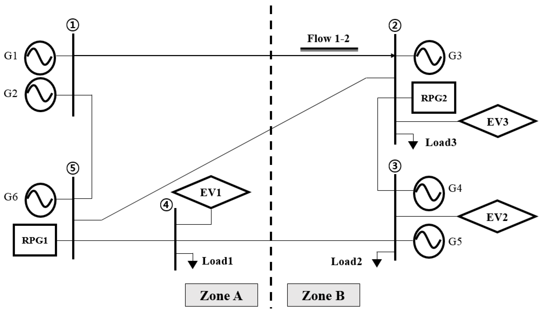
The proposed method was verified through case studies on a renewable power generator and a modified PJM 5-bus system with added EVs. The system is shown in Figure 2.

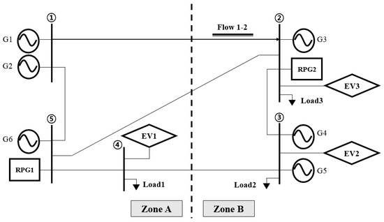
Figure 2. Modified PJM 5-bus system diagram.

The simulated system was composed of two zones. Only the power flow in the transmission line from node 1 to node 2 reached the maximum capacity among the transmission lines between Zones A and B. Therefore, the case studies considered the constraint only for transmission line 1–2, whose flow limit was 60 MW. The zonal aggregated sensitivities were $H_{1–2,a,t}^{FRU}=H_{1–2,a.t}^{FRD}=H_{1–2,a,t}^{EVRD}=0.4846$ and $H_{1–2,b,t}^{FRU}=H_{1–2,b,t}^{FRD}=H_{1–2,b,t}^{EVRU}=-0.0463$. Table 1 presents the characteristics of the conventional generator applied in the case studies, and Table 2 presents the sensitivity of the flow along transmission line 1–2 at each node.

Table 1. Conventional generator characteristics.

Generator	Min (MW)	Max (MW)	Ramp Rate (MW/min)	Offer Price ($/MWh)	Initial Output
G1	0	80	4	10	50
G2	0	80	4	10.1	25
G3	0	60	1	8	60
G4	0	160	1	25	160
G5	0	160	1	30	50
G6	0	100	1	15	100

Table 2. Sensitivity matrix of line 1–2.

	${\mathit{H}}_{1–2,1,\mathit{t}}$	${\mathit{H}}_{1–2,2,\mathit{t}}$	${\mathit{H}}_{1–2,3,\mathit{t}}$	${\mathit{H}}_{1–2,4,\mathit{t}}$	${\mathit{H}}_{1–2,5,\mathit{t}}$
Sensitivity	0.6	−0.08	−0.04	0.12	0.3

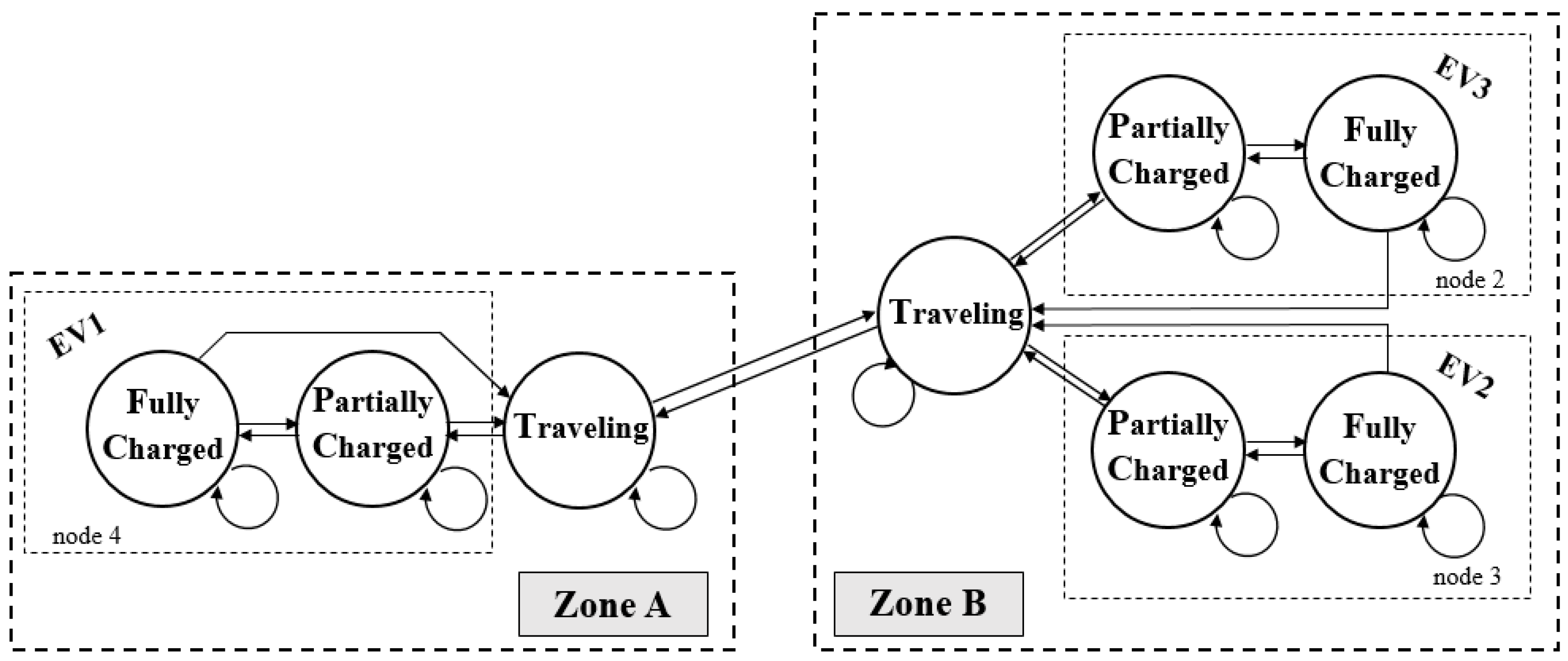
For all case studies, the regulating reserve and contingency reserve were not considered to concentrate on the FRP effect. Thus, only energy and the FRP were included. See Appendix A for versions of the above equations when reserves are included. The offer price of resources that provide ramping capability was excluded. A multiple-interval time-coupled dispatch model was applied to the simulation. This is an improvement over a single-interval dispatch model. Case studies were conducted regarding four dispatch time intervals of 5 min in series. EVs were assumed to be able to supply power to the system and to only be charged by the system. In addition, EVs were assumed to only be an FRU resource, not an FRD resource. The VOLL was assumed to be 3500 $/MWh. The problems of the case studies were solved using the GAMS 23.5/CPELX software (IBM, Armonk, NY, USA). Figure 3 presents all EV states that can exist through the Markov chain. EVs operated only at nodes 2, 3, and 4.

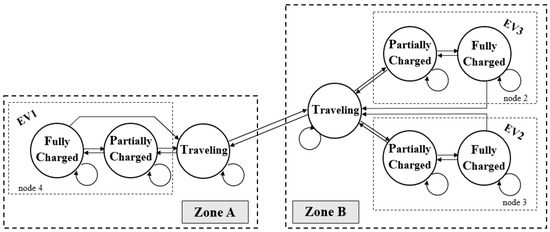
Figure 3. Markov chain applied to the case study.

The battery capacity of an individual EV was assumed to be 75 kWh, and the number of EVs in the test system was assumed to be 1500, which was assumed to represent a 1% EV penetration rate. At every time interval, the EV states changed according to the transition probability between the states. EVs were only applied as FRU resources in the fully charged or partially charged states, when connected with the system. η⁺ = 0.95, η⁻ = 0.98 and ε_ini = 0.7, ε_req = 0.8 were assumed. η⁺ and η⁻ indicate the discharging and charging coefficients of an EV, respectively. ε_ini represents the mean value of the remaining energy of each EV at T1. In addition, ε_req represents the required energy level of an EV at the end of the dispatch time. Figure 4 and Figure 5 show the results under these conditions.

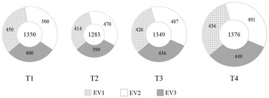
Figure 4. Number of parked EVs for an EV market penetration rate of 1%.

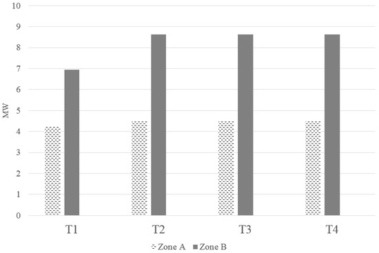
Figure 5. Discharging power of available EV fleets for an EV market penetration rate of 1%.

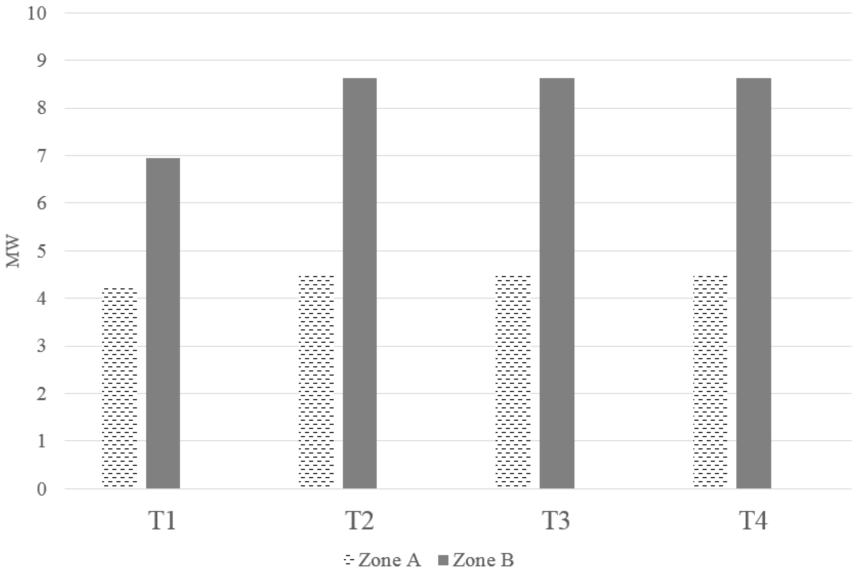
The number of parked EVs changed according to the time interval, which affected the available discharging capacity that could be secured from the EVs. Even though the number of parked EVs in the EV1 fleet at T1 was less than that of the EV2 fleet, more EVRU could be procured from the EV1 fleet. This is because even though the EV2 fleet contained more parked EVs, the EV1 fleet had higher available capacity considering the charged state of each EV. At T2–T4, even though the number of parked EVs changed with time, the applicable charging capacity was reached. Thus, the system operator could utilize the maximum available capacity supplied by the EV fleets for system operation at T2, T3, and T4.

4.1.1. Low Variability in Renewable Power—Case (a)

Case (a) was considered as the baseline of the case studies. The input data provided in Table 3 were applied. The results when EVs were and were not applied as an FRU resource were compared. The EV charge and discharge capacities were based on the pre-calculated values shown in Figure 4. Furthermore, the transmission constraint was considered in all cases. The results are presented in Table 4.

Table 3. Load and renewable data.

		T1	T2	T3	T4	T5	T6
Load (MW)		498	504	513	501	507	510
Renewable output (MW)	Low variability (a)	68	70	74	72	68	64
	High variability (b)	68	76	70	71	66	60

Table 4. Dispatch cleared products in case (a).

		EV, No Utilization for FRU (a)-1 Operating Cost: $11,009				EV, Utilization for FRU (a)-2 Operating Cost: $10,933
		Cost Saving: $76 (0.69%)
(MW)		T1	T2	T3	T4	T1	T2	T3	T4
G1	Energy	51.09	59.49	59.51	53.5	54.51	59.52	59.04	58.86
	FRU	6	0	0	9	1.83	0	1.05	0
	FRD	0	0	12	0	0	0	12	0
G2	Energy	5	0	0	0	5	0	0	0
	FRU	0	0	0	9	0	0	0	2.53
	FRD	0	0	0	0	0	0	0	0
G3	Energy	60	60	60	60	60	60	60	60
	FRU	0	0	0	0	0	0	0	0
	FRD	0	10	0	0	0	10	0	0
G4	Energy	155	160	155	150	155.64	160	159.26	154.26
	FRU	5	0	5	10	4.36	0	0.74	5.74
	FRD	0	10	0	0	0	10	0	0
G5	Energy	55	58.51	62.96	67.96	52.19	57.19	58.11	58.50
	FRU	10	10	10	10	10	10	10	10
	FRD	0	10	0	0	0	10	0	0
G6	Energy	100	100	99.13	100	100	100	100	100
	FRU	0	0	0	0	0	0	0	0
	FRD	10	10	0	0	10	10	0	0
EV1	Energy	0.52	−0.53	0.51	−0.52	0.52	−0.53	0.51	−0.52
	EVRU	x	x	x	x	0	0	0	0
EV2	Energy	1.61	−1.64	0.68	−0.69	0.89	−0.9	0.86	−0.88
	EVRU	x	x	x	x	2.59	5.21	3.45	5.19
EV3	Energy	1.79	−1.82	1.22	−1.25	1.25	−1.28	1.21	−1.24
	EVRU	x	x	x	x	2.22	5.59	3.1	5.55

Operating costs were reduced by applying EVs as an FRU resource. This is because the FRU capacity of the existing generator was replaced by EVs. The comparatively cheap G1 exhibited a high ramp rate. Table 4 indicates that G1 was used as an FRU resource and to generate energy to satisfy the ramp requirement of the system in case (a)-1. However, when EVs were applied as an FRU resource in case (a)-2, the EV2 and EV3 fleets were dispatched as FRU resources from T1 to T4. Therefore, the power generation of G1 could be used as energy instead of as an FRU resource, which reduced the relatively expensive power generation of G5. Thus, the total operating cost was reduced.

4.1.2. High Variability in Renewable Power—Case (b)

The normal loads for case (b) and (a) were the same; however, the change in renewable power increased. If the variability in renewable power increases, the variability in net load also increases, along with the ramp requirement of the system. In case (b)-1, EVs were not applied as an FRU resource; in case (b)-2, they were. For case (b)-1, a local shedding of 1.19 MW occurred at T1 of L3. With the set of a conventional generator, load shedding occurred because the ramp requirement was not satisfied owing to the high variability in renewable power. In case (b)-2, the increased ramp requirement was satisfied because EVs were applied as an FRU resource. Table 5 presents the dispatch results for cases (b)-1 and (b)-2. In case (b)-2, load shedding did not occur because EVs were applied as an FRU resource. This considerably reduced the operating cost compared to case (b)-1.

Table 5. EV dispatch results for case (b).

		EV, No Utilization for FRU (b)-1 Operating Cost: $12,457				EV, Utilization for FRU (b)-2 Operating Cost: $10,956
		Cost Saving: $1501 (12.05%)
(MW)		T1	T2	T3	T4	T1	T2	T3	T4
EV1	Energy	1.49	−1.52	0.53	−0.54	1.49	−1.52	1.44	−1.47
	EVRU	x	x	x	x	0	0	0	0
EV2	Energy	1.8	−1.84	0.68	−0.7	1.8	−1.84	1.75	−1.78
	EVRU	x	x	x	x	1.67	6.15	2.57	6.09
EV3	Energy	1.79	−1.82	1.22	−1.25	1.79	−1.82	1.73	−1.77
	EVRU	x	x	x	x	1.69	6.13	2.58	6.08

4.1.3. EV Market Penetration Rate Increase—Case (c)

The change with increased EV penetration was analyzed. The results were presented in Table 6. For case (a)-2, EVs were applied as an FRU resource. The EV penetration rates were 1%, 2%, and 3%; for cases (a)-2, (c)-1, and (c)-2, respectively.

Table 6. Operating cost and load shedding results for case (c).

EV Penetration Rate	Operating Cost	Load Shedding
1% (a)-2	$10,933	x
2% (c)-1	$10,941	x
3% (c)-2	$13,002	T2, L3 1.76 MW

When the EV penetration rate was 1%, the number of EVs was assumed to be 1500. Thus, a 1% increase in the penetration rate was equivalent to an increase of 1500 in the number of EVs. The charging load of EVs increases with the number of EVs; thus, the total load ultimately increases. According to the assumptions of the case studies, EVs should charge 10% of their batteries within four time intervals. Therefore, increasing the EV penetration rate by 1% increases the charging energy by 11.25 MWh.

The results showed that the operating cost of case (c)-1 increased slightly compared to that in case (a)-2. When the EV penetration rate was increased by 1%, the additional energy required for charging was 11.25 MWh, and the average offer price from G1 to G6 was approximately $16.3/MWh. Thus, the additional cost of charging the EVs through a generator was approximately $45. However, the actual increase in operating cost was smaller than this because the increased number of EVs was utilized as an FRU resource. As the EVs that could be applied as an FRU resource increased, the FRP capacity managed by a relatively cheap generator (e.g., G1) could be applied as energy. This decreased the energy produced by expensive generators, which reduced the total operating cost.

The operating cost in case (c)-2 was considerably higher than that in case (a)-2. This was because of the large increase in the charging load and the occurrence of load shedding at T2 of L3. When the EV penetration rate was above 3%, the total load (including the EV load) deviated from the range that could be managed by the system.

4.1.4. Necessity of Considering the Transmission Constraint—Case (d)

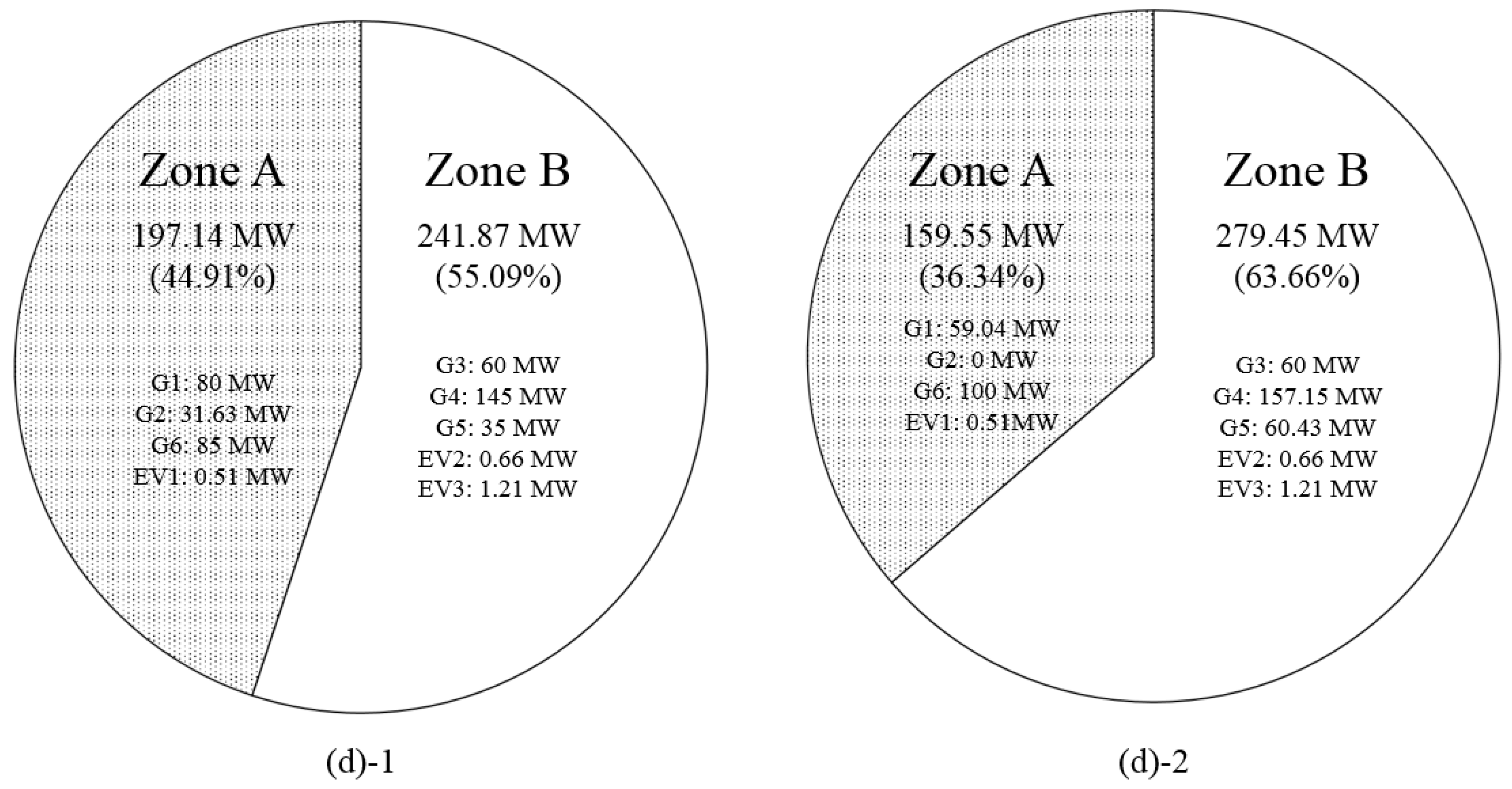
Table 7 presents the results when the transmission constraint was and was not considered (cases (d)-1 and (d)-2, respectively). Figure 6 shows the power generation for cases (d)-1 and (d)-2.

Table 7. Dispatch cleared products for case (d).

		Network Constraint Not Considered (d)-1 Operating Cost: $10,150				Network Constraint Considered (d)-2 Operating Cost: $10,933
(MW)		T1	T2	T3	T4	T1	T2	T3	T4
G1	Energy	67.55	80	80	80	54.51	59.52	59.04	58.86
	FRU	0	0	0	0	1.83	0	1.05	0
	FRD	0	0	12	0	0	0	12	0
G2	Energy	5	16.5	31.63	41.42	5	0	0	0
	FRU	0	0	12	9	0	0	0	2.53
	FRD	0	0	0	0	0	0	0	0
G3	Energy	60	60	60	60	60	60	60	60
	FRU	0	0	0	0	0	0	0	0
	FRD	10	10	0	0	0	10	0	0
G4	Energy	155	150	145	140	155.64	160	159.26	154.26
	FRU	5	0	0	10	4.36	0	0.74	5.74
	FRD	10	10	0	0	0	10	0	0
G5	Energy	45	40	35	30	52.19	57.19	58.11	58.5
	FRU	10	10	0	10	10	10	10	10
	FRD	10	10	0	0	0	10	0	0
G6	Energy	95	90	85	80	100	100	100	100
	FRU	5	0	0	0	0	0	0	0
	FRD	10	10	0	0	10	10	0	0
EV1	Energy	0.52	−0.53	0.51	−0.52	0.52	−0.53	0.51	−0.52
	EVRU	1	0	0	0	0	0	0	0
EV2	Energy	0.68	−0.69	0.66	−0.7	0.89	−0.9	0.86	−0.88
	EVRU	0	0	0	0	2.59	5.21	3.45	5.19
EV3	Energy	1.25	−1.28	1.21	−1.24	1.25	−1.28	1.21	−1.24
	EVRU	0	0	0	0	2.22	5.59	3.1	5.55

Figure 6. Comparison of power generation by zone at T3.

In case (d)-1, where the transmission constraint was not considered, the power output from Zone A generators changed without limit as the total power generation increased. However, in case (d)-2, which considered the transmission constraint, the limits of transmission line capacity implied that Zone A generators could not produce more than a certain power output. As shown in Figure 6, the ratio of the power generation at T3 in Zone A was 44.91% in case (d)-1 and 36.34% in case (d)-2. When the transmission constraint was not considered, even if a large amount of power was generated in Zone A, the physical transmission constraints limited the power that could flow to Zone B. In this situation, the power of Zone A was wasted, or there was a shortage of power in Zone B. Thus, for reliable system operation and practical available dispatch results, the transmission constraint should be considered.

For case (d)-2, the operating cost was higher than that of case (d)-1. However, such a result is not practical. Because G1 is a relatively cheap generator, it was dispatched to the maximum in T2–T4 for case (d)-1. However, the results of case (d)-2 showed that the G1 generator could not be dispatched to the maximum owing to the transmission constraint.

In case (d)-1, EV fleets were mostly not used for FRU. In case (d)-2, however, EVRU was actively used. Of course, EV fleets could be applied in case (d)-1 as FRU; however, they were not applied because the conventional generators could be used for FRU. When constraint conditions were considered in case (d)-2, the system operator procured FRU through the EV2 and EV3 fleets in Zone B. These results indicate that the FRU capacity should be calculated by considering the transmission constraint to derive a practical result and increase EV utilization.

5. Conclusions

This paper proposed a method of applying EVs as an FRP in a power system including renewable energy. The charging and discharging capacities between the grid and EV were considered. To consider the movement and location of EVs and the changes in their charged states, a probabilistic method of calculating battery capacity was propose to make EVs applicable as an FRU resource. Case studies were conducted to understand the impact of applying EVs as an FRU resource. The simulation results revealed that applying EVs as an FRU resource reduced the operating cost, and it was more effective in situations with high variability due to renewable power. The results demonstrated the effectiveness of considering the transmission constraint to increase the utilization of EVs as an FRU resource. Future work will involve applying the proposed approach to actual systems and including reserve products. In addition, methods of calculating the ramp requirement capacity more precisely will be developed.

Appendix A.1. Objective Function

$$Min{\displaystyle \sum _{t=t_0}^{t_s}\left(C{G}_i+CE{V}_x+CL{S}_t\right)}$$

(A1)

$$C{G}_i={\displaystyle \sum _{i\in I}\left[C_i^{energy}{p}_{i,t}+C_i^{FRU}FR{U}_{i,t}+C_i^{FRD}FR{D}_{i,t}+{\displaystyle \sum _{w\in W}{C}_i^w{r}_{i,t}^w}\right]}$$

(A2)

$$CE{V}_x={\displaystyle \sum _{x\in X}\left[C_x^{dis}pe{v}_{x,t}^{dis}-C_x^{cha}pe{v}_{x,t}^{cha}+C_x^{EVRU}EVR{U}_{x,t}+C_x^{EVRD}EVR{D}_{x,t}\right]}$$

(A3)

$$CL{S}_t=VOLL\times L{S}_t$$

(A4)

Appendix A.1. Objective FunctionAppendix A.2. Constraints

-

Resource Capability

$$\forall t,\forall i:{{\displaystyle p}}_{i,t}+{\displaystyle \sum _{w\in W}{{\displaystyle r}}_{i,t}^w}+FR{U}_{i,t}\le {{\displaystyle p}}_i^{\max }-{\varphi }_{i,t}\left(p_{i,t}^{\max }-p_{i,t}^{reg,\max }\right)$$

(A5)

$${{\displaystyle \forall t,\forall i:p}}_{i,t}-{{\displaystyle r}}_{i,t}^{reg}-{{\displaystyle FRD}}_{i,t}\ge {{\displaystyle p}}_{i,t}^{\min }-{\varphi }_{i,t}\left(p_{i,t}^{\min }-p_{i,t}^{reg,\min }\right)$$

(A6)

-

System Reserve

$$\forall t:{\displaystyle \sum _{z\in Z}{{\displaystyle r}}_{z,t}^{reg}}\ge {{\displaystyle R}}_{system,t}^{reg}$$

(A7)

$$\forall t:{\displaystyle \sum _{z\in Z}\left\{{{\displaystyle r}}_{z,t}^{reg}+{{\displaystyle r}}_{z,t}^{spin}\right\}}\ge {{\displaystyle R}}_{system,t}^{reg}+{{\displaystyle R}}_{system,t}^{spin}$$

(A8)

$$\forall t:{\displaystyle \sum _{z\in Z}\left\{{\displaystyle \sum _{w\in W}{{\displaystyle r}}_{z,t}^w}\right\}}\ge {\displaystyle \sum _{w\in W}{{\displaystyle R}}_{system,t}^w}$$

(A9)

-

Zonal Reserve

$$\forall t,\forall z:{\displaystyle \sum _{i\in I,z}{{\displaystyle r}}_{i,t}^{reg}}\ge {{\displaystyle r}}_{z,t}^{reg}$$

(A10)

$$\forall t,\forall z:{\displaystyle \sum _{i\in I,z}\left\{{{\displaystyle r}}_{i,t}^{reg}+{{\displaystyle r}}_{i,t}^{spin}\right\}}\ge {{\displaystyle r}}_{z,t}^{reg}+{{\displaystyle r}}_{z,t}^{spin}$$

(A11)

$$\forall t,\forall z:{\displaystyle \sum _{i\in I,z}\left\{{\displaystyle \sum _{w\in W}{r}_{i,t}^w}\right\}}\ge {\displaystyle \sum _{w\in W}{r}_{z,t}^w}$$

(A12)

-

Reserve Up and FRU/FRD

$$\begin{array}{l}\forall t,\forall l:F_{l,t}\left(P_t,E{V}_t,D_t\right)+{\displaystyle \sum _{z\in Z}\left\{r_{z,t}^{reg}\cdot H_{l,z,t}^{reg}\right\}}+{\displaystyle \sum _{z\in Z}\left\{FR{U}_{i,z,t}\cdot H_{l,z,t}^{FRU}\right\}}-{\displaystyle \sum _{z\in Z}\left\{FR{D}_{z,t}\cdot H_{l,z,t}^{FRD}\right\}}\\ +{\displaystyle \sum _{x\in X,z}\left\{EVR{U}_{x,t}\cdot H_{l,z,t}^{EVRU}\right\}}-{\displaystyle \sum _{x\in X,z}\left\{EVR{D}_{x,t}\cdot H_{l,z,t}^{EVRD}\right\}}-H_{l,LC,t}\cdot R_{Mar}^{reg}\le F_{l,t}^{N.\max }\end{array}$$

(A13)

-

Reserve Down and FRU/FRD

$$\begin{array}{l}\forall t,\forall l:F_{l,t}\left(P_t,E{V}_t,D_t\right)-{\displaystyle \sum _{z\in Z}\left\{r_{z,t}^{reg}\cdot H_{l,z,t}^{reg}\right\}}+{\displaystyle \sum _{z\in Z}\left\{FR{U}_{z,t}\cdot H_{l,z,t}^{FRU}\right\}}-{\displaystyle \sum _{z\in Z}\left\{FR{D}_{z,t}\cdot H_{l,z,t}^{FRD}\right\}}\\ +{\displaystyle \sum _{x\in X,z}\left\{EVR{U}_{x,t}\cdot H_{l,z,t}^{EVRU}\right\}}-{\displaystyle \sum _{x\in X,z}\left\{EVR{D}_{x,t}\cdot H_{l,z,t}^{EVRD}\right\}}+H_{l,LC,t}\cdot R_{Mar}^{reg}\le F_{l,t}^{N.\max }\end{array}$$

(A14)

-

Contingency

$$\forall t,\forall l:F_{l,t}\left(P_t,E{V}_t,D_t\right)-Q_{z,t}\cdot H_{l,z,t}^C+D_{z,t}^{spin}\cdot {\displaystyle \sum _{z\prime \in Z}\left\{r_{z\prime ,t}^{spin}\cdot H_{i,z\prime ,t}^{spin}\right\}}+D_{z,t}^{supp}\cdot {\displaystyle \sum _{z\prime \in Z}\left\{r_{z\prime ,t}^{supp}\cdot H_{i,z\prime ,t}^{supp}\right\}}\le F_{l,t}^{C.limit}$$

(A15)

References

- Holttinen, H.; Meibom, P.; Orths, A.; Lange, B.; O’Malley, M.; Tande, J.O.; Estanqueiro, A.; Gomez, E.; Söder, L.; Strbac, G.; et al. Impacts of large amounts of wind power on design and operation of power systems, results of IEA collaboration. Wind Energy 2011, 14, 179–192. [Google Scholar] [CrossRef]
- Eftekharnejad, S.; Vittal, V.; Heydt, G.T.; Keel, B.; Loehr, J. Impact of increased penetration of photovoltaic generation on power systems. IEEE Trans. Power Syst. 2013, 28, 893–901. [Google Scholar] [CrossRef]
- Gul, T.; Stenzel, T. Variability of Wind Power and Other Renewables: Management Options and Strategies; International Energy Agency: Paris, France, 2005. [Google Scholar]
- Kunz, H.; Hagens, N.J.; Balogh, S.B. The Influence of Output Variability from Renewable Electricity Generation on Net Energy Calculations. Energies 2014, 7, 150–172. [Google Scholar] [CrossRef]
- Banakar, H.; Luo, C.; Ooi, B.T. Impacts of wind power minute-to-minute variations on power system operation. IEEE Trans. Power Syst. 2008, 23, 150–160. [Google Scholar] [CrossRef]
- Makarov, Y.V.; Loutan, C.; Ma, J.; De Mello, P. Operational impacts of wind generation on California power systems. IEEE Trans. Power Syst. 2009, 24, 1039–1050. [Google Scholar] [CrossRef]
- Kassakian, J.G.; Schmalensee, R.; Desgroseilliers, G.; Heidel, T.D.; Afridi, K.; Farid, A.; Grochow, J.; Hogan, W.; Jacoby, H.; Kirtley, J.; et al. The Future of the Electric Grid; Massachusetts Institute of Technology (MIT): Cambridge, MA, USA, 2011. [Google Scholar]
- Lannoye, E.; Flynn, D.; O’Malley, M. Evaluation of power system flexibility. IEEE Trans. Power Syst. 2012, 27, 922–931. [Google Scholar] [CrossRef]
- Kirby, B.; Beuning, S.J.; Connolly, K.; Dangelmaier, L.; Rosso, A.D.; Frost, W.; Grant, W.; Guttromson, R.; Henson, B.; John, E.; et al. Operating Practices, Procedures, and Tools; North American Electric Reliability Corporation (NERC): Princeton, NJ, USA, 2011. [Google Scholar]
- EnerNex. NSP Wind Integration Study Prepared for Xcel Energy; EnerNex.: Knoxville, TN, USA, 2014. [Google Scholar]
- Wu, C.; Hug, G.; Kar, S. Risk-limiting economic dispatch for electricity markets with flexible ramping products. IEEE Trans. Power Syst. 2016, 31, 1990–2003. [Google Scholar] [CrossRef]
- Wang, B.; Hobbs, B.F. Real-time markets for flexiramp: A stochastic unit commitment-based analysis. IEEE Trans. Power Syst. 2016, 31, 846–860. [Google Scholar] [CrossRef]
- Wang, C.; Luh, P.B.S.; Navid, N. Ramp requirement design for reliable and efficient integration of renewable energy. IEEE Trans. Power Syst. 2017, 32, 562–571. [Google Scholar] [CrossRef]
- Navid, N.; Rosenwald, G. Market solutions for managing ramp flexibility with high penetration of renewable resource. IEEE Trans. Sustain. Energy 2012, 3, 784–790. [Google Scholar] [CrossRef]
- Xu, L.; Tretheway, D. Flexible Ramping Products: Revised Draft Final Proposal; California ISO: Folsom, CA, USA, 2014. [Google Scholar]
- Navid, N. Ramp Capability Product Design for MISO Markets; MISO: Saint Paul, MN, USA, 2013. [Google Scholar]
- MISO. Ramp Management. Available online: https://www.misoenergy.org/WhatWeDo/MarketEnhancements/Pages/RampManagement.aspx (accessed on 2 November 2017).
- Chen, R.; Wang, J.; Botterud, A.; Sun, H. Wind power providing flexible ramp product. IEEE Trans. Power Syst. 2017, 32, 2049–2061. [Google Scholar] [CrossRef]
- Cui, M.; Zhang, J.; Wu, H.; Hodge, B.M.; Ke, D.; Sun, Y. Wind power ramping product for increasing power system flexibility. In Proceedings of the Transmission and Distribution Conference and Exposition (T&D), Dallas, TX, USA, 3–5 May 2016. [Google Scholar]
- Zhang, B.; Kezunovic, M. Impact on power system flexibility by electric vehicle participation in ramp market. IEEE Trans. Smart Grid 2016, 7, 1285–1294. [Google Scholar] [CrossRef]
- Gottwalt, S.; Schuller, A.; Flath, C.; Schmeck, H.; Weinhardt, C. Assessing load flexibility in smart grids: Electric vehicles for renewable energy integration. In Proceedings of the Power and Energy Society General Meeting (PES), Vancouver, BC, Canada, 21–25 July 2013. [Google Scholar]
- Kempton, W.; Tomić, J. Vehicle-to-grid power implementation: From stabilizing the grid to supporting large-scale renewable energy. J. Power Sources 2005, 144, 280–294. [Google Scholar] [CrossRef]
- White, C.D.; Zhang, K.M. Using vehicle-to-grid technology for frequency regulation and peak-load reduction. J. Power Sources 2011, 196, 3972–3980. [Google Scholar] [CrossRef]
- Pavić, I.; Capuder, T.; Kuzle, I. Value of flexible electric vehicles in providing spinning reserve services. Appl. Energy 2015, 157, 60–74. [Google Scholar] [CrossRef]
- Ortega-Vazquez, M.A.; Bouffard, F.; Silva, V. Electric vehicle aggregator/system operator coordination for charging scheduling and services procurement. IEEE Trans. Power Syst. 2013, 28, 1806–1815. [Google Scholar] [CrossRef]
- Tomić, J.; Kempton, W. Using fleets of electric-drive vehicles for grid support. J. Power Sources 2007, 168, 459–468. [Google Scholar] [CrossRef]
- Tang, D.; Wang, P. Nodal Impact Assessment and Alleviation of Moving Electric Vehicle Loads: From Traffic Flow to Power Flow. IEEE Trans. Power Syst. 2016, 31, 4231–4242. [Google Scholar] [CrossRef]
- Khodayar, M.E.; Wu, L.; Li, Z. Electric vehicle mobility in transmission-constrained hourly power generation scheduling. IEEE Trans. Smart Grid 2013, 4, 779–788. [Google Scholar] [CrossRef]
- Sun, Y.; Zhong, J.; Li, Z.; Tian, W.; Shahidehpour, M. Stochastic scheduling of battery-based energy storage transportation system with the penetration of wind power. IEEE Trans. Sustain. Energy 2017, 8, 135–144. [Google Scholar] [CrossRef]
- Chen, Y.; Gribik, P.; Gardner, J. Incorporating post zonal reserve deployment transmission constraints into energy and ancillary service co-optimization. IEEE Trans. Power Syst. 2014, 29, 537–549. [Google Scholar] [CrossRef]
- Zheng, T.; Litvinov, E. Contingency-based zonal reserve modeling and pricing in a co-optimized energy and reserve market. IEEE Trans. Power Syst. 2008, 23, 277–286. [Google Scholar] [CrossRef]
- Chatterjee, D.; Hansen, C.; Howard, J.; Larson, K.; Li, S.; Merring, B.; Trotter, K.; Wang, C.; Fogarty, J. Ramp Capability Integration Technical Work; MISO: Saint Paul, MN, USA, 2016. [Google Scholar]
- International Energy Agency. Global EV Outlook: Two Million and Counting; International Energy Agency: Paris, France, 2017. [Google Scholar]
- Arias, N.B.; Tabares, A.; Franco, J.F.; Lavorato, M.; Romero, R. Robust joint expansion planning of electrical distribution systems and EV charging stations. IEEE Trans. Sustain. Energy 2017, PP, 1. [Google Scholar] [CrossRef]
- Guo, J.; Zhang, Y.; Chen, X.; Yousefi, S.; Guo, C.; Wang, Y. Spatial stochastic vehicle traffic modeling for VANETs. IEEE Trans. Intell. Transp. Syst. 2017, PP, 1–10. [Google Scholar] [CrossRef]
© 2017 by the authors. Licensee MDPI, Basel, Switzerland. This article is an open access article distributed under the terms and conditions of the Creative Commons Attribution (CC BY) license (http://creativecommons.org/licenses/by/4.0/).