A Data Analysis Technique to Estimate the Thermal Characteristics of a House ^†

Abstract

Almost one third of the energy is used in the residential sector, and space heating is the largest part of energy consumption in our houses. Knowledge about the thermal characteristics of a house can increase the awareness of homeowners about the options to save energy, for example by showing that there is room for improvement of the insulation level. However, calculating the exact value of these characteristics is not possible without precise thermal experiments. In this paper, we propose a method to automatically estimate two of the most important thermal characteristics of a house, i.e., the loss rate and the heat capacity, based on collected data about the temperature and gas usage. The method is evaluated with a data set that has been collected in a real-life case study. Although a ground truth is lacking, the analyses show that there is evidence that this method could provide a feasible way to estimate those values from the thermostat data. More detailed data about the houses in which the data was collected is required to draw stronger conclusions. We conclude that the proposed method is a promising way to add energy saving advice to smart thermostats.

1. Introduction

More and more thermostats function as smart devices, with features like large color screens, the ability to learn usage patterns, and internet connection, which offers the possibility of remote control and online information. Often, these features are also used to provide the user with insight into the domestic energy usage (e.g., [1,2,3]). Smart thermostats can contribute to more economic energy use in two ways. On the one hand, they can control the heating system in an economic manner, for example by not heating the house if they detect that nobody is at home. On the other hand, they play an important role in making the persons in the house aware of their energy usage, for example by informing them where and when the energy is used and how it would be possible to reduce the usage. Doing so, they encourage users to change their heating behaviour or to improve the energy characteristics of the houses, e.g., by insulation.

To let smart thermostats contribute to the reduction of domestic energy usage, an important challenge is to provide it with the intelligence needed to analyze the thermal characteristics of a house. This could provide the basis for comparisons with other users and tailored advice about measures to reduce energy usage. In this paper, we present an approach to derive those characteristics based on monitoring devices and an analysis method for interpreting the measured data. The work described in this paper uses data of gas consumption and the indoor and outdoor temperatures over time to derive some important thermal characteristics of a house.

To analyze the energy usage of a house, often so-called heating ‘degree day’ methods are used (e.g., [4,5,6,7,8,9]). These methods allow estimating the heating demand of a house based on the difference between the indoor and outdoor temperature. In this paper, the ‘degree day’ method is used as the basis for a method that is able to estimate the thermal characteristics of a house such as heat loss rate and heat capacity.

The main research question in this paper is whether the heating characteristics of a house can be estimated based on temperature and gas usage data, given an imperfect and incomplete data set. It is important to emphasize that in this work we are trying to estimate the heating characteristics of a house. An exact calculation of these parameters would only be possible based on precise thermal experiments or detailed information about the design and construction of the building, which is not possible in our use case in which a smart thermostat automatically estimates these thermal characteristics. This paper, therefore, presents a heuristic approach based on data that can be collected by a thermostat.

To evaluate our heuristic, we use a data set of house temperatures and gas usage that has been collected via a smart thermostat. We evaluate whether the capacity C of a house that is estimated by our method is positively correlated with its size, and whether the calculated loss rat $\epsilon$ is correlated with both the assumed insulation level of the house based on its building year and its size. Unfortunately, our data set does not contain information about the actual thermal characteristics of the houses. We, therefore, formulate a number of hypothesis about relations between thermal characteristics of the houses and expected properties of the houses in our dataset. We compare this with some data in the literature about the relation of gas usage and house characteristics.

This paper is an extension of earlier work [10]. In the current paper, the proposed approach is improved and evaluated using a richer database of empirical data. In the remainder of this paper, we first discuss related work on energy usage in domestic buildings and the role of the thermostat in energy usage. In Section 3, we provide the theoretical background in the form of some basic thermodynamic theories. Next, in Section 4, we introduce our approach for analyzing building characteristics based on monitoring temperature and gas usage by a thermostat. In Section 5, the data that is used to validate our method is described. Section 6 shows the results of applying our approach to the data. Finally, the paper is concluded with a discussion in Section 7 and a conclusion.

2. Related Work

2.1. Energy Usage for Heating Buildings

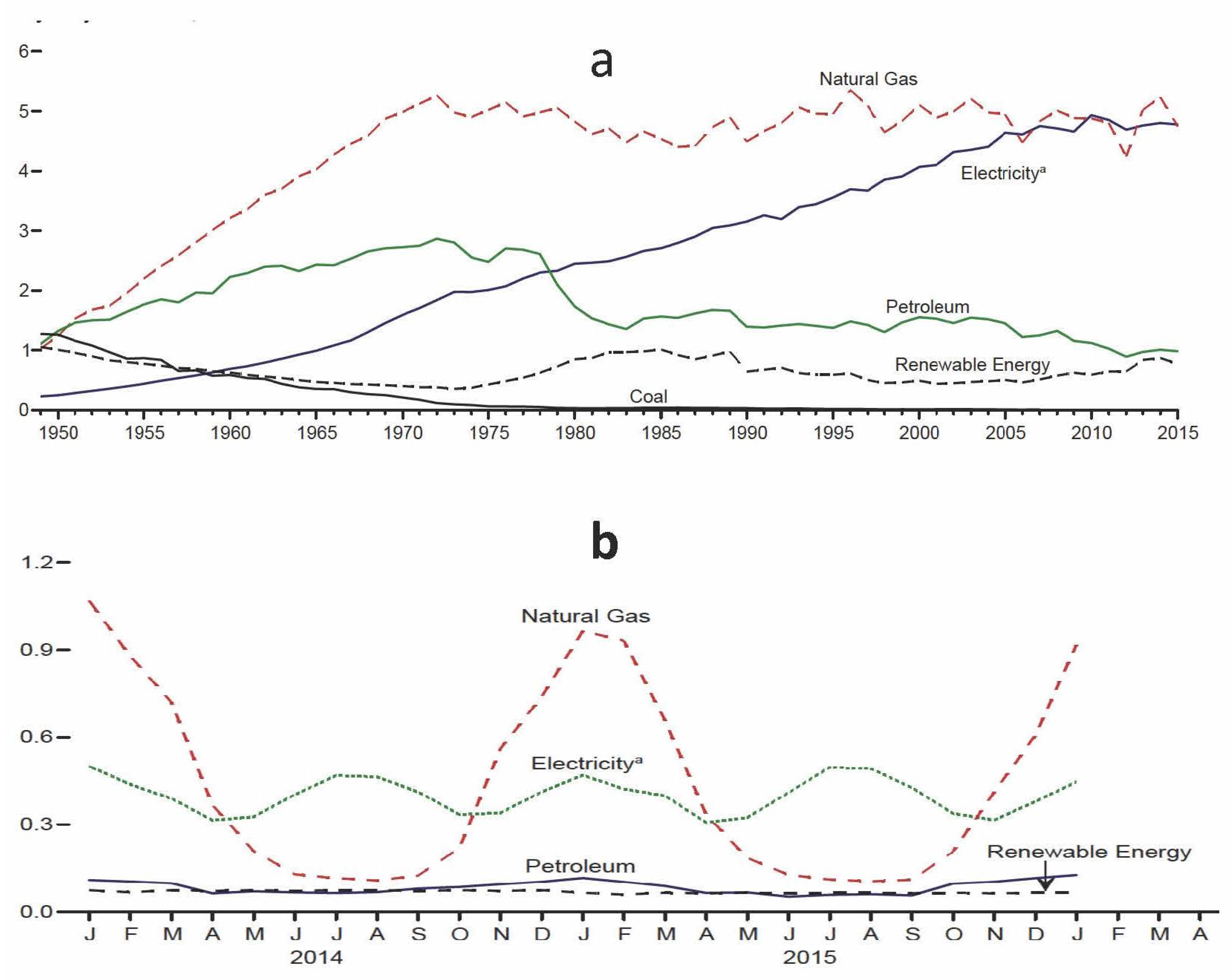
The use of fossil fuels, which leads to significant environmental problems like climate change and global warming, is to a large extent related to the heating of buildings. According to data published by U.S. Energy Information Administration, in 2015, about 40% of the total U.S. energy consumption was used in residential and commercial buildings. Figure 1 shows the major source of energy used in the buildings in the U.S. (A: Annually from 1950; B: monthly for 2014 and 2015). As can be seen in Figure 1a, the usage of natural gas is almost constant in the last four decades (with some variations). However, by looking at it on a more detailed level (Figure 1b), we can see that there is a clear seasonal pattern in the natural gas usage, which shows that it is mainly used for heating purposes. It is therefore relevant to see how the energy used for heating in domestic buildings can be reduced.

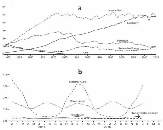
Figure 1. Energy major sources in U.S. (a) yearly data from 1949; (b) monthly data of 2014 and 2015, Source: U.S. Energy Information Administration (EIA).

Building characteristics play an important role in the energy usage of households. There are different researchers that study the effect of different factors on energy usage for heating in a building. One of the most important aspects is the size of the house. Many studies find a positive correlation between this aspect and the energy usage in a house [11,12,13]. In [13], an analysis is provided of the relation between the usage of gas and electricity on the one hand and the technical specifications of the houses and the demographic characteristics on the other hand. The study is based on data of more than 300,000 Dutch homes and their occupants. A positive correlation of around 0.29 is found between the log of the gas usage and the log of the dwelling area in m².

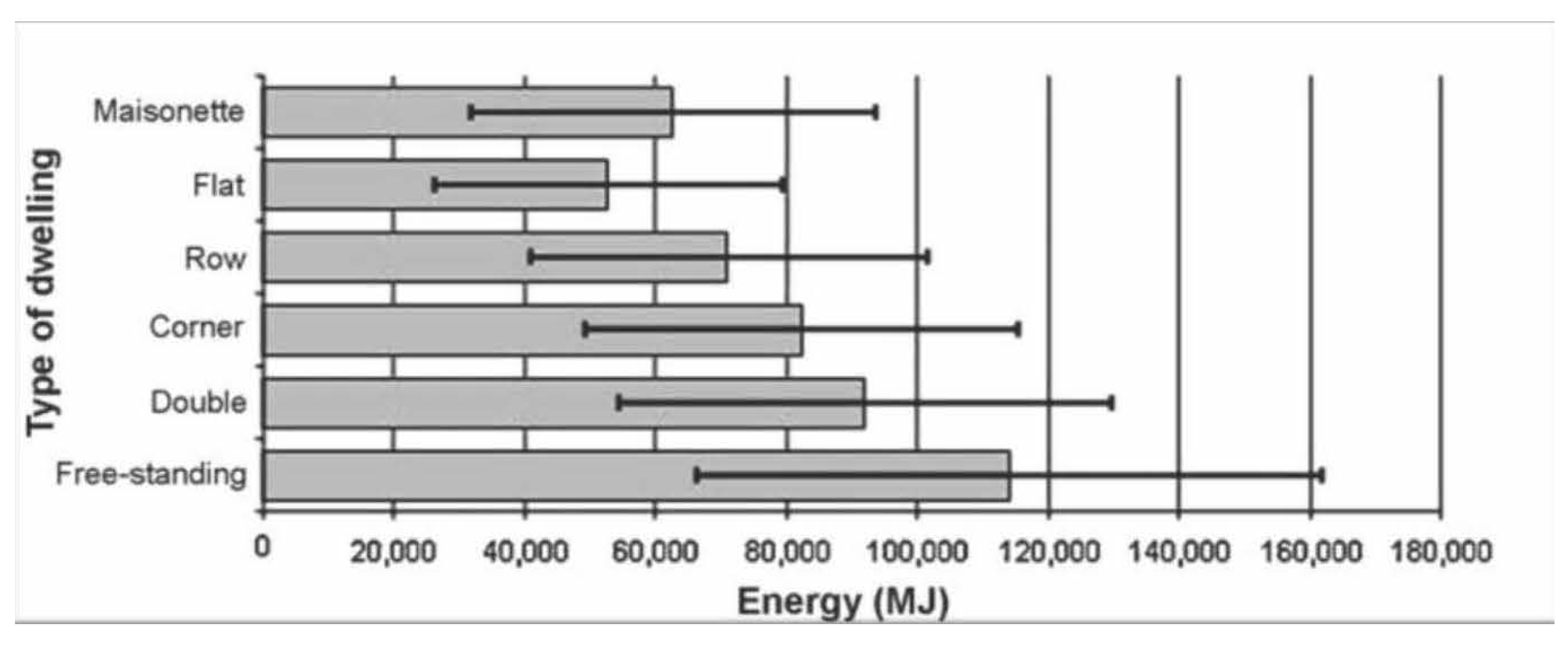
The type of dwelling is another important factor. In [11], another analysis is provided of the effect of different factors on energy usage for heating. It discusses the respective importance of building characteristics, household characteristics and occupant behaviour on energy use for space and water heating in the Netherlands. The study shows that occupant characteristics and behaviour significantly affect energy use (4.2% of the variation in energy use for heating), but the building characteristics determine the largest part of the energy use in a dwelling (42% of the variation in energy use for heating). It describes that, in the residential sector, in addition to size and location, the type of dwelling is the other important feature that affects its energy consumption. Figure 2 shows the annual consumption of per type of house, which resulted from analysis of the energy consumption of 15,000 houses across the Netherlands.

Figure 2. Average and standard deviation for energy use (MJ/Year) per type of dwelling (adapted from [11]).

Another important factor that affects the amount of energy usage in a house is the building year. In general, newer houses use less energy. Figure 3 shows the annual average gas consumption of around 300,000 houses in the Netherlands based on the building year [13]. This figure indicates the variation in total average energy use by building year. Gas usage for heating is clearly lower for more recent constructed buildings. The paper concludes that “relative to dwellings constructed in this century, we find that gas consumption increases with the ages of dwellings”. Age is significantly related to gas usage, where the regression estimate between older buildings (<1960) are around 0.6, and newer buildings (>1990) around 0.14.

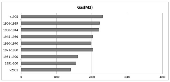
Figure 3. Annual energy consumption and constrution year (redrawn from [13]).

The use of a thermostat also plays a role in the energy usage in buildings. However, it can affect the usage in two directions. According to [11], the presence of a thermostat has a negative impact on energy use, in contrast to houses with temperature control in the form of radiator taps. This could be explained by the fact that, in dwellings with a thermostat, occupants are more aware of the temperature in the home and therefore tend to turn it on more often that those without a thermostat. In contrast, Hirst and Goeltz [14] found that a thermostat is also important for energy savings, as it can control the heating system in a manner that it minimizes the energy consumption without decreasing the comfort level seriously.

The set point of a thermostat has a large effect on the energy usage. Calculations by Tommerup et al. [15] based on single-family houses in Denmark revealed that the increase in energy consumption is about 10% per degree of indoor temperature. Some papers (e.g., [16]) show that it is possible to provide advice on the optimal set point for a house based on data of the indoor temperature only. The method measures the effect of lowering the set point of the houses and to what extent a high set point affects the energy usage in a house.

Therefore, it is relevant to see how thermostats can be improved and extended in such a way that they have a more certain positive contribution to energy saving. One of the ways to achieve this is making the thermostat aware of the causes of high energy usage. For example, both behavioural aspects and building characteristics can play a role. By differentiating those causes, a smart thermostat can provide better tailored suggestions for energy reduction. In order to build such a smart thermostat, a thermodynamic model of the house should be built.

2.2. Effect of Solar Radiation

The effect of solar radiation on the heating demand can be significant, especially if the house is designed to gain as much radiation as possible. In such buildings, windows, walls, and floors are made to collect, store, and distribute solar energy in the form of heat in the colder periods. The key to designing such a building is to best take advantage of the local climate performing an accurate site analysis. Elements to be considered include window placement and size, and glazing type, thermal insulation, thermal capacity, and shading [17]. For a review of the techniques and technologies to use the solar radiation for space heating, please read [18]. Technically, direct-gain systems can utilize (i.e., convert into “useful” heat) up to 65–70% of the energy of solar radiation that strikes the aperture or collector.

However, in practice, most houses are not designed in such a way. In regular houses, the effect of irradiation on the heating load is on the order of 10–20% of the heat demand [19]. Moreover, this effect is the largest in the summer time in which no additional heating is required, and the smallest in the colder winter times.

2.3. Related Products

There are a number of commercial smart thermostats available, mainly with the aim to automate the heating and sometimes also to provide personalized home heating advice to households. The most important ones are discussed below.

Nest by Google [20] is a programmable, and learning thermostat that optimizes heating and cooling of homes and businesses to conserve energy. It is based on a machine learning algorithm. The Auto-Schedule feature automatically generates a schedule based on temperature changes users make. Moreover, Nest can then learn people’s schedules, at which temperature they are used to and when. Using built-in sensors and phones’ locations, it can shift into energy saving mode when it realizes nobody is at home. The Nest has an embedded motion sensor on the wall-mounted unit that detects the movement of occupants within a certain range. If the Nest does not sense movement for about two hours, it goes into “Auto-Away” mode, which automatically adjusts the temperature to a predefined level to use less energy.

Joulo [16] uses a model-based approach for providing advice about the thermal characteristics of a house. It does not use data of consumption of the heating system in the calculations but only indoor temperatures. This technique is based on a number of strong assumptions. The first assumption is that the thermostat has a single set-point throughout the day, which is in most real households not the case. Another (even stronger) assumption is that energy produced by the heating system in all time intervals is always the same. Even if the heating system has just two modes (on/off), this usually is not a valid assumption, since the system may be ‘on’ just for part of an interval.

‘Toon’ [21] , is a smart thermostat developed by Quby and mainly distributed by the Dutch utility company Eneco. With this smart thermostat, customers can get detailed insight into their energy consumption. It shows the power that is currently used, the daily energy usage for both gas and electricity, and the overall usage. An important feature is the comparison with comparable households [22]. It is estimated that customers can save between 5.1% and 6.1% on their yearly gas usage with this thermostat.

Although smart thermostats can help people to save energy in buildings, there is some resistance against using them, especially due to security vulnerabilities, like [3].

3. Theoretical Background

Heat transfer between a building and the outside causes changes in its inside temperature. This section discusses some theoretical background about basic thermodynamic theories. With these basic thermodynamics, we can find out how the temperature of the house changes in response to the addition of energy in any period of time. The theoretical background that we discuss concerns gas-based heating and the relation to outdoor temperature. The central concepts that characterize a house are heat loss rate $\epsilon$ (depending on insulation level of the house) and heat capacity C of the house (depending on construction material and the volume of the house).

3.1. Degree Day

Degree day based energy analysis is a well-known approach to quantify the relationship between energy usage and the difference between the outdoor and indoor temperature of a building (e.g., [5,7,8,9]). Through this, it is possible to approximate the heating and cooling demand of a building. The original definition of degree days, DD, is for a complete day (24 h), but it is possible to define degree days for any period of time ([6]):

$$DegreeDa{y}_{PeriodA}=D{D}_{PeriodA}={\int }_{PeriodA}(T_{in}-T_{out})dt.$$

(1)

The formula above is a differential equation based on continuous values for T, where T is represented in centigrade. However, since in practical applications, the values of indoor and outdoor temperature ($T_{in}$ and $T_{out}$) are not available continuously, this equation can be transformed into a discrete variant:

$$D{D}_{PeriodA}=\sum _{PeriodA}(T_{in}-T_{out})\Delta t.$$

(2)

Here, the smaller the period length $\Delta$t, the higher the accuracy.

3.2. Heat Gain

Buildings gain heat in several ways (e.g., residents, appliances, solar radiation, heating system).

• Residents always are warmer than the house, since the temperature of a regular house is always less than 37 °C. As a result, there is a continuous heat transfer from the people who live there to the indoor air.
• Electric appliances also produce heat. However, since those factors together form a relatively small part of heat gained by a house (usually less than 20%), in this work, it is ignored.
• Solar radiation can be a noticeable part of the gained heat of a building during a sunny day. In this paper, this source of heat is ignored as well. As a result, this method is more applicable for houses that do not receive much radiation from the sun during the heating season.
• For most of the houses in colder areas, a heating system is the main source of heat gain during winter time. Different buildings use different kinds of heating systems. For the regular gas-based heating systems, one form of energy (chemical) is transformed into thermal energy. The performance rate $\rho$ of a system is an important parameter that directly affects the provided amount of thermal energy:

  $$EnergyProvided=\rho \times InputEnergy.$$

  (3)

Both Energy Provided and Input Energy are represented in kWh. The input energy refers to the amount of energy that is provided to the heating system. Many modern meters can measure the amount of gas used on an hourly basis. Based on this, it is straightforward to calculate the energy that is in a particular volume of natural gas; the energy content of one cubic meter of natural gas is about 10 kWh.

3.3. Heat Loss

During cold winter days, houses lose energy to the outside in several ways. Some of this energy loss is due to conduction and infiltration that depend on the long-term characteristics of the house. Here, conduction refers to heat transfer that happens because of the adjacency of walls, roof, etc. of a house and air outside. Infiltration is the unintentional introduction of outside air into a building, typically through cracks in a building envelope. Ventilation means changing or replacing air in a building to decrease temperature or to replenish fresh air. For automated ventilation systems, this is a constant factor. However, for non-automated ventilation systems, this does not happen continuously, and it depends on the residents’ behavior (how frequently and for how long they keep the windows open) and is not a characteristic of the house.

Aggregating conduction, infiltration and ventilation, the amount of energy lost in a period is a linear function of the amounts of degree days for that period. Thus, in general, for any period of time, we have:

$$EnergyLos{s}_{PeriodA}={\epsilon }_{PeriodA}\times D{D}_{PeriodA}={\epsilon }_{PeriodA}\times {\int }_{PeriodA}(T_{in}-T_{out}).$$

(4)

Here, $\epsilon$ is the heat loss rate. It depends on the insulation level of the area of the house in contact with the outside: the walls, windows, floor, and roof. For each period of time, the energy loss of a house per time unit with indoor temperature $T_{in}$ and (lower) outdoor temperature $T_{out}$ is proportional to the temperature difference $T_{in}$ − $T_{out}$ between indoor and outdoor temperatures. The proportion factor is by definition the heat loss rate $\epsilon$.

For the periods of time that energy loss is only caused by conduction, infiltration and automated ventilation (not manual), energy loss just depends on the long-term characteristics of the house. As a result, the loss rate values for such periods are almost the same, and it is considered a characteristic of the house. In general, the better the insulation level of the house, the lower the loss rate. In contrast, the loss rates for the periods that manual ventilation is happening are not the same and depend on the rate of airflow. In general, the loss rate for a period with manual ventilation is higher than the loss rate for a period when no manual ventilation is taking place. In the rest of this paper, $\epsilon$ without a subscript refers to the loss rate as a characteristic of the house, and with a subscript refers to the loss rate during a special period of time.

3.4. Thermal Capacity C

The thermal capacity C is a characteristic that describes the mass of a building that can store heat. In addition to the size of the house, there are other factors that determine the thermal capacity, notably the construction material and furniture. The thermal capacity determines the amount of energy that has to be added to the building to allow for an increase in temperature of 1 degree. For a building, one can roughly say that its thermal capacity has a correlation with its size (in the sense of volume in m³): the larger the house, the higher value of C.

Thus, the thermal capacity is defined as the ratio of the amount of heat energy added to an object and the resulting increase in temperature of the object: the amount of energy needed to increase the indoor temperature is proportional to the difference $\Delta T_{in}$ in indoor temperature. The proportion factor C is the heat capacity. Thus, this concept shows how the temperature of the house will change due to the addition of energy:

$$NetEnergyAdded=C\times \Delta T_{in}.$$

(5)

Here, the Net Energy Added of the house is the amount of energy added to the building during a particular period of time minus the energy loss in that period. Moreover, $\Delta T_{in}$ shows the difference in temperature of the house at the beginning and the end of the considered period.

4. Proposed Approach

In Section 3, a simple thermodynamic model of a building was described. In this section, we use the model introduced above to estimate the values of loss rate ($\epsilon$) and thermal capacity (C) based on collected data of the inside and outside temperature ($T_{in}$, $T_{out}$) and the gas usage.

To do that, the focus of this approach is on relatively short periods of time during which the indoor temperature has a downward, upward or stable trend. It is important to notice that the shortest length of periods for such an analysis is a few hours. This has two reasons. First, the gas usage is collected on an hourly basis, so we do not have information about the gas usage during periods shorter than one hour. Secondly, after using some gas in the heating system, it takes some time to transfer this energy to the house environment. Thus, by shortening the periods of usage, we do not have an accurate estimation of the provided energy during those periods.

In the remainder of this section, the different types of periods (with downward, upward or stable temperature trends) are discussed, and it is explained how to use data of such periods to relate the loss rate $\epsilon$ and the capacity C. We do this by deriving for each type of period linear equations that have $\epsilon$ and C as unknown variables. Then, we explain how we can calculate the loss rate and capacity by combining data from at least two different types of periods.

4.1. Cooling Periods

A cooling period refers to a period of time in which the house is not heated via the heating system and its temperature is decreasing. In this type of period, the net energy added to the house is equal to the energy loss of the house. Therefore, Equation (5) can be rewritten in this form (note that $\Delta T_{in}$ is negative in case of decreasing indoor temperature):

$$EnergyLoss=-C\times \Delta T_{in}.$$

(6)

By combining Equations (4) and (6) , we derive the following equation for cooling periods:

$$C\times \Delta T_{in}=-\epsilon \times DD.$$

(7)

This shows that in a cooling process the indoor temperature decrease ($\Delta T_{in}$) is proportional to the difference between indoor and outdoor temperature as calculated in $DD$. The proportion factor $\epsilon$/C is called the cooling rate, indicated by $\mu$. Thus, during a cooling period, the following equation holds:

$$\mu =\frac{\epsilon }{C}=\frac{-\Delta T_{in}}{DD}.$$

(8)

To calculate $\mu$ from Equation (8) we just need to have the dynamics of $T_{in}$ and $T_{out}$; for any cooling period, it is possible to do that by using the indoor and outdoor temperature data.

4.2. Heating Periods

For periods of time that heating energy is provided and the indoor temperature is increasing, the provided energy is used for both compensating the energy loss and also for increasing the temperature. Thus, by combining Equations (4) and (5) , we get the following equation:

$$ProvidedEnergy=Energyloss+EnergyforIncreasingTemperature=\epsilon \times DD+C\times \Delta T_{in}.$$

(9)

4.3. Periods with Stable Temperature

In periods that no significant change in temperature takes place (i.e., $\Delta T_{in}$ = 0), the provided energy is only needed to compensate the energy loss. Therefore, the second part of Equation (9) will be zero, and the equation can be simplified to:

$$ProvidedEnergy=\epsilon \times DD.$$

(10)

In these periods, the provided energy is independent of the capacity C. Therefore, for any period with a stable temperature, an estimation of $\epsilon$ can be obtained.

4.4. Combining Different Periods

Given that each of the types of periods result in different equations that relate $\epsilon$ and C, it is possible to estimate the values of $\epsilon$ and C if we have data for at least two different types of periods. For example, when we have data for both cooling periods and heating period, we can combine Equations (8) and (9) to derive values for $\epsilon$:

$$\epsilon =\frac{ProvidedEnergy}{DD+\frac{\Delta T_{in}}{\mu }}.$$

(11)

The value of C can be calculated by rewriting the definition of $\mu$ in Equation (8) :

$$C=\frac{\epsilon }{-\Delta T_{in}}\times DD.$$

(12)

In a similar way, we can calculate $\epsilon$ and C based on the combination of measurements during other types of periods.

In our approach, we decide on a case by case basis which types of periods are used to estimate $\epsilon$ and C for a specific house. The decision is based on the availability and the quality of the data that is available for the specific house.

More specifically we just count on the periods for which indoor temperature has the same trend (down, up, constant) for more than two hours. For each house, if there are more than five periods with downward trends, and more than five periods with upward trends, then the resulting formulas of cooling and heating periods are used to calculate $\epsilon$ and C. In the cases that the number of periods for cooling or heating periods is less than five, the resulting formula from periods with stable temperature is replaced.

5. Data

Our method described above is validated using actual data of both temperature and gas usage. The data was collected by a smart thermostat development company, Quby. Data was collected from 22 January 2015 until 17 August 2015. During this period, data was collected from 99 Dutch households that have a smart thermostat (called Toon) installed and agreed to be part of this data collection. Since the focus of this work is on colder periods, we just used data of January, February, and March. For this study, the following variables collected from the thermostat were used:

• Indoor temperature: actual indoor temperature as measured by the thermostat with the precision of 0.5 C. The indoor temperature has a value for every minute in degree Celsius.
• Gas use: total gas used, in liters (0.001 m³) for every hour.

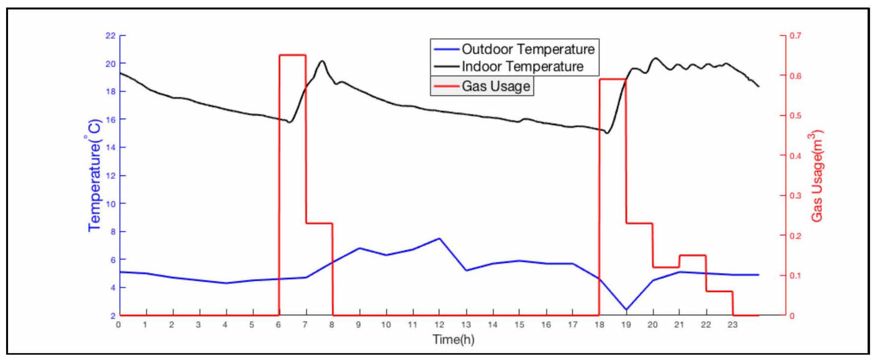
An example of the temperature data is provided in Figure 4. The data from the thermostat was combined with general information about the characteristics of the household. These were used for validation and include:

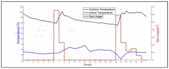
Figure 4. Gathered data from one sample house for 24 h.

• The construction period of the house, divided into the following six groups: before 1946, between 1946 and 1964, between 1965 and 1974, between 1975 and 1987, between 1988 and 1999, after 1999;
• The total floor area of the house in square meters;
• The type of household, which is one of the following: apartment, terraced, semidetached or detached. For terraced houses, it is mentioned if it is on the corner or not;
• The geographical location of the houses. We have access to a 4-digit zip code, which shows the neighborhood area of the house. An overview is provided in Figure 5. Red pins show the location of houses. As shown, most of the houses are located in the big cities in the southern half of the Netherlands.
  

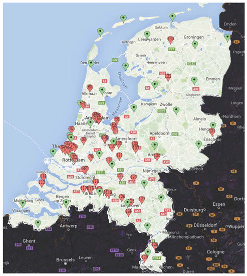  Figure 5. Location of houses and weather stations. Each red pin depicts the location of a house in our dataset. In addition, green pins show the location of weather stations, which are used to find the outdoor temperature.

The dataset was used in an anonymized way. A unique number identifies each house. Table 1 shows an overview of the general information of the houses.

Table 1. General information of the houses in the dataset.

Feature	Description
Living Area	Minimum : 45 m2
	Maximum : 400 m2
Building Year	Category	#
	Older than 1946	28
	Between 1946 and 1965	9
	Between 1966 and 1975	10
	Between 1976 and 1988	17
	Between 1989 and 2000	22
	After 2000	13
Type of House	Type	#
	Apartment	10
	Terraced, Not corner	48
	Terraced, On corner	17
	Semi detached	17
	Detached	6
	Unknown	1

In the proposed approach, the outdoor temperature is a critical measurement. However, it is missing from this data because the thermostat does not directly measure this value. Therefore, this data was acquired by using the publicly available dataset of The Royal Netherlands Meteorological Institute (KNMI), which contains the weather/climate data measurements of 35 weather stations. The locations of these stations are shown in Figure 5 by green pins. To derive the difference between the indoor and outdoor temperature for each house, the gathered data by its thermostat is combined with temperature data of the nearest weather station.

A disadvantage of this method is that actual outdoor temperature for houses that are not close to a weather station might differ from the temperature measured by the station. To examine to what extent this issue is problematic, we calculated the difference of the measured temperature of three randomly selected weather stations with their nearest weather station. We found out that, on average, there is a difference of 0.9 °C, while, at some time points, the difference might briefly go up to 6 °C. It should be noticed that, in our approach, the distance of the houses to the closest weather station is less than the distance between two stations. We, therefore, assume that the error in our experiments is less.

6. Experimental Results

The main research question in this paper is whether the heating characteristics of a house can be estimated based on temperature and gas usage data, given an imperfect and incomplete data set. As a matter of fact, evaluating this method requires precise and expensive experiments to measure the exact value of thermal characteristics of houses, which is not possible in our case. To overcome this problem, a number of hypotheses were formulated to study the results based on the available information in the used dataset:

Hypothesis 1.

The calculated capacity C of a house is positively correlated with its volume or size in terms of total floor area of all floors (a large house requires more energy to be heated).

Hypothesis 2.

The calculated loss rate ε is correlated with insulation level of the house. As the data set does not contain specific information about this, we operationalize this hypothesis in the following ways:

-

Hypothesis a. The calculated loss rate ε is correlated with the building year of the house: the older the house, the higher the loss rate.

-

Hypothesis b. The calculated loss rate ε is correlated with the type of the house: the more detached a house, the higher the loss rate.

Hypothesis 3.

The calculated loss rate ε is correlated with size of the house. It means that the larger houses usually have more walls and lose more energy in comparison to smaller ones.

In the next subsections, we first describe how the data was processed and then we show the relation between estimated thermal characteristics and the known properties of houses. It should be emphasized that the aim of this method is to validate the estimations, and not to derive the non-thermal characteristics (e.g., size) of the buildings.

6.1. Data Processing and Selection

In order to calculate the $\mu$ during cooling periods, it is necessary to analyze time intervals in which no energy is added by the heating system. For each house, the set of periods or time intervals with no gas usage and a downward trend for the indoor temperature are extracted. To get rid of delays in the heating and metering system (it takes some time before the heating system has transferred the heat to the house environment through the hot water in the radiators, and the gas meter only provides data per hour), the first hour of each period was removed. For each cooling period, the cooling ratio ($\mu$) was calculated based on Equation (8). As an example, a cooling period is visible in Figure 4 from 1 h to 6 h.

Given the number of time intervals in which cooling takes place, for each house, several estimated values for the cooling down rate are calculated, some of which are outliers. Our assumption is that this is caused by external factors, for example, windows or doors are opened and the energy loss is increased significantly. Under this condition, Equation (8) does not apply anymore, and the value of the calculated rate will be much higher than the actual one (These observations can possibly still be used as a technique in smart thermostats, e.g., to alert the residents that probably a window or door was open for hours).

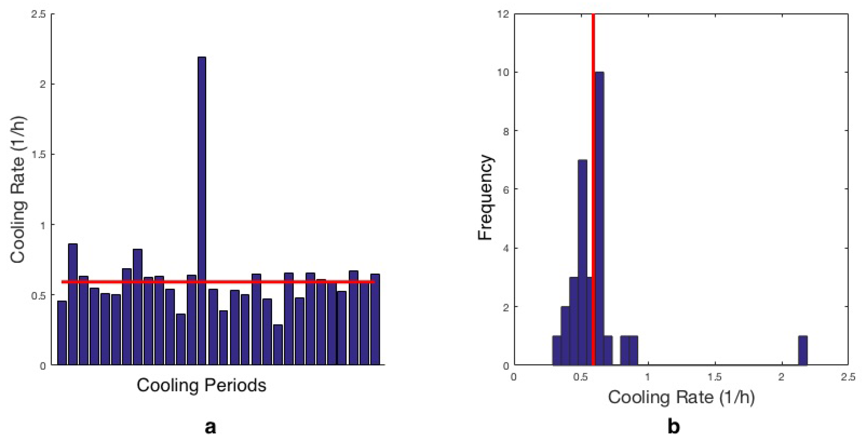
Figure 6a shows the calculated values of cooling rate ($\mu$) for different cooling periods for a sample house, and Figure 6b shows the histogram of them. A possible explanation for the difference in the calculated cooling rate for different cooling periods can be that the situation of each period is different. For instance, during some cooling periods, maybe some heating energy still remains in the radiators and is transferred into the house.

Figure 6. (a) calculated values of cooling rate ($\mu$) for different cooling periods for a sample house; (b) the histogram of calculated values of cooling rate ($\mu$).

The cooling rate that is caused by conduction and infiltration (not manual ventilation) is a fixed characteristic of a building. The challenge is to derive this value from the values that were calculated based on the different cooling periods. To do that, we have to identify which of the cooling rates result from periods with and without manual ventilation, or are affected by solar irradiation. To remove the effect of these outliers caused by periods with manual ventilation (loosing energy) or by periods in which there was another source of heat (like sunshine), the 25% lowest and 25% highest values are ignored. The average of others is taken as the resulted estimation of $\mu$. In Figure 6, this value is depicted by a red line.

For periods with invariant temperatures, an estimation of $\epsilon$ can be obtained. For an example, we refer to Figure 4 again, in which can be seen that the period between 20 h and 23 h is a period with invariant temperature. Such periods are common for houses in which the heating system is controlled by a thermostat. The thermostat keeps the temperature stable for a specific period of time by turning the heating system on and off frequently.

Given the number of such intervals, several values for $\epsilon$ are estimated. For the same reasons as explained above, we have used a quintile of 50% of these values for the calculation.

6.2. Relation between Thermal Capacity and Size

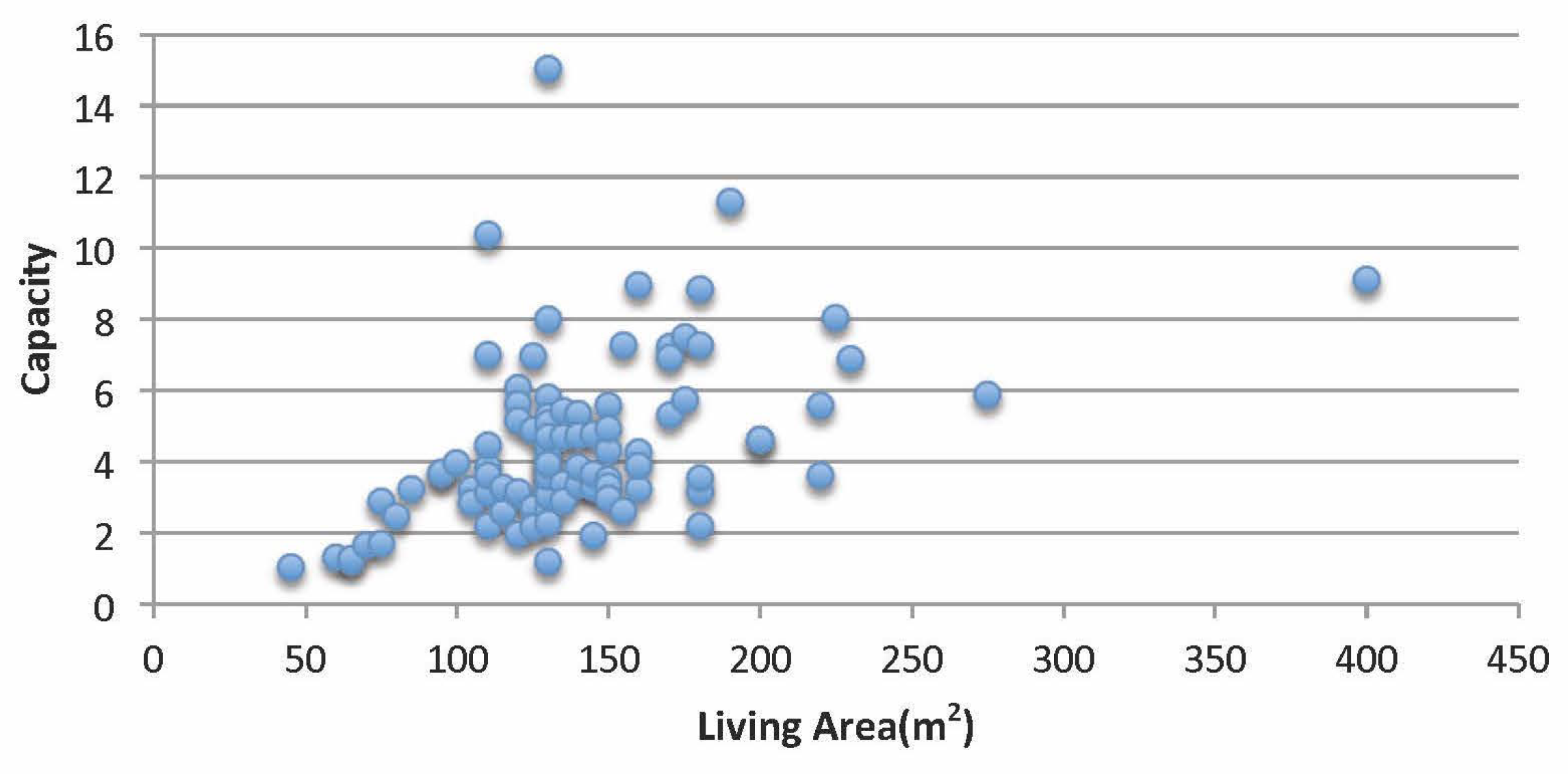
To investigate the first hypothesis, Figure 7 is generated that shows the relation between the estimated capacity and the size of houses according to our data set.

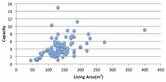
Figure 7. Relation between size of the house and estimated value for thermal capacity.

As it is seen in this graph, in general, it holds that, for larger houses, a higher value for C is estimated. We have done a Pearson correlation (Pearson correlation is a measure of linear correlation between two variable X and Y. The value of “correlation coefficient” is in the range of [−1, +1], where +1 is a total positive linear relation, 0 is no linear relation and $-1$ is total negative linear relation) test on the results. It shows that there is a significant correlation (correlation coefficient = 0.42515, p-value = 0.000127) between the living area of houses and the estimated thermal capacity.

6.3. Relation between Loss Rate and Building Year

The building year of a house is also important in predicting energy use. In general, newer houses use less energy as they are better insulated, also expected by the theory [11]. The age of the houses was found to have a positive correlation to energy use. Similar results were found by Leth Petersen and Togeby [23] in Denmark and Liao and Chang [24] in the USA.

As it was explained in Section 5, we do not have the exact building year of houses, but have houses in 6 categories (before 1946, between 1946 and 1964, between 1965 and 1974, between 1975 and 1987, between 1988 and 1999, after 1999). Based on Hypothesis 2a, it is expected that older houses lose more energy, and thus have a higher loss rate. Figure 8 shows the average and standard deviation of estimated loss rate of houses categorized based on their building year.

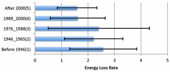
Figure 8. Relation between building year of the house and estimated value for heat loss rate.

In general, it seems to be the case that newer houses have a smaller loss rate. The results are in line with Hypothesis 2a, except for houses built between 1976 and 1988. However, this category has the highest standard deviation. The high value for the average in this category may be caused by a few outliers.

To check the correlation between the category of building year and the loss rate, we performed Spearman’s correlation test [25], which is a measure of rank correlation. The results ($\rho$ = −0.326, p-value = 9.8208 × ${10}^{-4}$) show a small negative correlation, which is statistically significant and means that the estimated energy loss rate for the newer buildings (higher value for building year) is lower than older buildings.

6.4. Relation between Loss Rate and Type of Houses

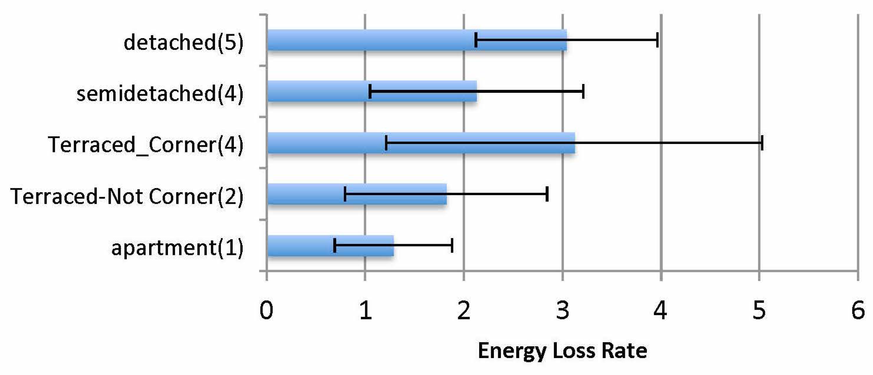
Figure 9 shows the relation between loss rate and type of house. Since for terraced houses we have information about whether it is on a corner or not, this category is split into two separate categories (terraced on corner, terraced not corner).

Figure 9. Relation between type of the house and estimated value for heat loss rate.

The depicted results in this graph point in the direction of hypothesis Hypothesis 2b. except for terraced houses that are located on the corner. It should be noted that this category of houses has the highest standard deviation.

To check the correlation between the type of building and its loss rate, Spearman’s correlation is done. The results (Rho = 0.373, p-value = 1.553 × ${10}^{-4}$) show a strong correlation.

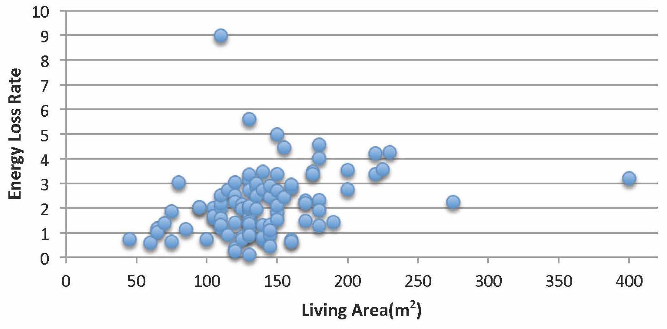
6.5. Relation between Loss Rate and Size

As a way to answer hypothesis Hypothesis 3, Figure 10 shows the relation between loss rate and the size of houses. As can be seen in this graph, in general, a larger loss rate is estimated for larger houses. We performed a Pearson correlation test and found out that there is a slight correlation, which is statistically significant (with a coefficient of 0.3183 and a p-value of 0.0014).

Figure 10. Relation between size of the house and estimated value for heat loss rate.

7. Discussion

We have proposed an approach in which a thermostat (or a mobile app that has access to data gathered by a thermostat) can provide advice based on an estimation of the main thermal characteristics of a house by using temperature data and gas usage data. This approach has been evaluated by analyzing a dataset of energy usage and inside temperature of 99 Dutch houses. As the data does not provide exact information about the thermal characteristics of those houses (i.e., a ground truth is not available), we have formulated some hypotheses about expected relations between the outcome of our approach and the available characteristics in our dataset (dwelling type, building year and living area).

In the analysis presented above, we have provided some evidence that the outcomes of our approach are in line with the expected characteristics of the considered houses. However, a more detailed study in which the actual characteristics of the buildings are known is required to validate our approach.

When we try to specifically assess the quality of our estimations, we can make a few remarks. First, with respect to the correlation between living area and capacity (Section 6.2), we find a correlation of around 0.43. It is difficult to estimate the actual capacity of a house, but the outcome that a house of 200 m² has more or less twice the capacity of a house with a living area of 100 m² seems not unrealistic, given the fact that most of the capacity is caused by the walls and floors of a house. With respect to the relations with the loss rate (Section 6.3,Section 6.4,Section 6.5), we could not find information in the literature about the relation between loss rate and building characteristics. However, we were able to find information about the relation between gas usage and building characteristics (see Section 2). If we consider that the gas usage can be explained up to 42% by building characteristics [11], we can assume that the relations between loss rate and building characteristics should be in the same direction as those between gas usage and building characteristics. The estimations of the loss rate per building year (Section 6.3) seems quite adequate and in line with [13], in which also is concluded that the gas usage for houses up to 1960 does not much differ, but that newer houses use less gas. The same holds for the relation between type of house and gas usage (Section 6.4), although here the comparison is hampered by the fact that the categories are slightly different. The quality of the estimation of the relation between loss rate and size (Section 6.5) is probably the most difficult one to assess. We find a slight correlation of around 0.32; in [13] a correlation of around 0.29 is found between the log of the dwelling size and the log of the gas usage. Overall, we tend to conclude that this correlation is not unrealistic.

8. Limitations

In general, we would like to mention that our approach is based on additional critical assumptions and that its correctness depends on the correctness of those. The following assumptions can thus be seen as limitations of our work:

• The temperature of the whole house is the same, which is an acceptable assumption just for small houses, like a studio. In larger houses, especially those with a separate office room, this might not be the case.
• The Degree-day based energy consumption approximation is adequate. We realize that it is a simple method. For having a more accurate model, it may be better to use more complex modeling techniques. Buildings with different thermal insulation levels at different sides of the building will have different base temperatures, which need to be factored into the simplified degree–day method for the determination of energy demand. However, for our use case, such an approach is less feasible.
• The heating system is the only important source of heating for the building. It means that the heat transfer from the body of residents to the house is ignored. This is acceptable if only a few persons live in the house. Similarly, as discussed in Section 2.2, we neglect the effect of solar radiation. This approach is therefore more applicable for areas that do not have much sun during the heating season, like northern countries of Europe. On the other hand, it should be noticed that solar irradiation has an effect just on (cooling and heating) periods that are occurring during sunny days. In our data set, we believe that those periods are to a large extent part of the outliers, and their effect is minimized by removing 25% of the lowest and 25% of the highest values before averaging (see Section 6.1).
• The performance of the heating system does not change notably. This assumption is true for most gas-based and electric heating systems. However, in the case of air source heat pumps, of which the performance is dependent on the outdoor temperature, this assumption is not true. However, by using some mathematical models (e.g., [26]), it is possible to estimate the performance for different moments and calculate the characteristics of the house based on that.
• Energy consumed by a heating system is only used for space heating. In some real cases, this assumption is not true, and the provided energy is used for both space and sanitation water heating. However, it may be possible to figure out in which periods the energy is also used for sanitation water heating. In [27], the summer data (when no space heating is done) is used to find a pattern for daily hot water usage in a house. This pattern is used to have an estimation of the fraction of the energy that is used for water heating.
• The outdoor temperature is collected from nearby weather stations. As discussed in Section 5, this might result in an inaccuracy. The best option to overcome this problem is to collect the outdoor temperature on the site. However, it would be possible to decrease the error by using interpolation techniques to combine the temperature of different weather stations.

In this paper, it is assumed that the only available data are indoor temperature, outdoor temperature and input energy of the heating system. However, by the spread of more modern thermostats, more data collected by the thermostat become available (e.g., the temperature of heating water at the beginning and the end of the circuit, the presence of residents and etc.). Future work can address different data analysis techniques for different types of available data. This can result in more complex and more accurate thermodynamic models.

As a consequence of the improved quality of thermal properties of buildings due to energy regulations, the overall energy use associated with building characteristics is decreasing, making the role of the occupant more important. Studies have shown that occupant behaviour might play a prominent role in the variation in energy consumption in different households, but the exact extent of such influence is unknown. The impact of the building’s thermal characteristics on space heating demand has been well studied. There is, however, little work done that incorporates the impact of user behavior [11]. A smart thermostat can learn the information about the energy consumption behaviour of residents. Interesting potential future research is to study the different ways to learn this information, and also to study techniques to use this information in the optimization of the energy consumption and the comfort level of residents.

9. Conclusions

The need and will for energy saving in the built environment are increasing. Private initiatives together with government intervention, new technologies for energy production, limiting energy consumption and raising social awareness on the rational use of energy will be essential in order to realize a sustainable energy future [28].

In this paper, an approach has been discussed that allows a smart thermostat to estimate some of the thermal characteristics of a house over time: heat loss rate and heat capacity. The proposed approach is based on degree-day analysis methods. The approach has been evaluated using a data set including data of a variety of houses of different types. This dataset is not complete. The approach turns out to be able to handle data with some extent of incompleteness. The analysis shows that there is evidence that our method provides a feasible way to estimate those values from the thermostat data. More detailed data about the houses in which the data was collected would be required to draw stronger conclusions. In addition, a more thorough evaluation of our heuristics should be done based on a data set in which the exact thermal characteristics of the houses are known.

The techniques proposed in this paper could be used to improve the awareness of users about the impact of the current state of their house on heating energy cost. The techniques can be used to add features to smart thermostats. One option is to provide feedback about thermal characteristics and the functioning of the heating system. By monitoring the estimated characteristic of the house over time, a probable malfunctioning in the heating system [29] can be distinguished from a high loss rate due to house characteristics. In the first case, a warning can be provided to check the heating system, while, in the latter case, advice can be given to check the frame of doors and windows for unwanted infiltrations. Another possibility is to encourage people to save energy, by allowing them to compare their energy use based on their behavior, compensated for the characteristics of their house. Another interesting possibility is to take dynamic energy prices, which are expected to be used in smart grid systems, into account in the calculations (cf. [30]). Together with calculations of the expected change in energy usage due to insulation measurements at the different times of the day, a more precise prediction of the financial savings can be provided.

References

- Ellis, C.; Scott, J.; Hazas, M.; Krumm, J. EarlyOff: Using house cooling rates to save energy. In Proceedings of the Fourth ACM Workshop on Embedded Sensing Systems for Energy-Efficiency in Buildings, Toronto, ON, Canada, 6 November 2012; pp. 39–41. [Google Scholar]
- Gao, P.X.; Keshav, S. SPOT: A smart personalized office thermal control system. In Proceedings of the Fourth International Conference on Future Energy Systems, Berkeley, CA, USA, 21–24 May 2013; pp. 237–246. [Google Scholar]
- Hernandez, G.; Arias, O.; Buentello, D.; Jin, Y. Smart Nest Thermostat: A Smart Spy in Your Home. Black Hat USA. 2014. Available online: https://pdfs.semanticscholar.org/f1aa/f326c8b2cb6a94fa105b9910125e61920714.pdf (accessed on 8 September 2017).
- Abdelaziz, O.; Shen, B. Cold climates heat pump design optimization. ASHRAE Trans. 2012, 118, 34. [Google Scholar]
- De Rosa, M.; Bianco, V.; Scarpa, F.; Tagliafico, L.A. Heating and cooling building energy demand evaluation; a simplified model and a modified degree days approach. Appl. Energy 2014, 128, 217–229. [Google Scholar] [CrossRef]
- Durmayaz, A.; Kadıoǧlu, M.; Şen, Z. An application of the degree-hours method to estimate the residential heating energy requirement and fuel consumption in Istanbul. Energy 2000, 25, 1245–1256. [Google Scholar] [CrossRef]
- Quayle, R.G.; Diaz, H.F. Heating degree day data applied to residential heating energy consumption. J. Appl. Meteorol. 1980, 19, 241–246. [Google Scholar] [CrossRef]
- Al-Homoud, M.S. Computer-aided building energy analysis techniques. Build. Environ. 2001, 36, 421–433. [Google Scholar] [CrossRef]
- Ueno, T.; Sano, F.; Saeki, O.; Tsuji, K. Effectiveness of an energy-consumption information system on energy savings in residential houses based on monitored data. Appl. Energy 2006, 83, 166–183. [Google Scholar] [CrossRef]
- Van der Ham, W.; Klein, M.; Tabatabaei, S.A.; Thilakarathne, D.J.; Treur, J. Methods for a Smart Thermostat to Estimate the Characteristics of a House Based on Sensor Data. Energy Procedia 2016, 95, 467–474. [Google Scholar] [CrossRef]
- Santin, O.G.; Itard, L.; Visscher, H. The effect of occupancy and building characteristics on energy use for space and water heating in Dutch residential stock. Energy Build. 2009, 41, 1223–1232. [Google Scholar] [CrossRef]
- Kavousian, A.; Rajagopal, R.; Fischer, M. Determinants of residential electricity consumption: Using smart meter data to examine the effect of climate, building characteristics, appliance stock, and occupants’ behavior. Energy 2013, 55, 184–194. [Google Scholar] [CrossRef]
- Brounen, D.; Kok, N.; Quigley, J.M. Residential energy use and conservation: Economics and demographics. Eur. Econ. Rev. 2012, 56, 931–945. [Google Scholar] [CrossRef]
- Hirst, E.; Goeltz, R. Comparison of actual energy savings with audit predictions for homes in the north central region of the USA. Build. Environ. 1985, 20, 1–6. [Google Scholar] [CrossRef]
- Tommerup, H.; Rose, J.; Svendsen, S. Energy-efficient houses built according to the energy performance requirements introduced in Denmark in 2006. Energy Build. 2007, 39, 1123–1130. [Google Scholar] [CrossRef]
- Rogers, A.; Ghosh, S.; Wilcock, R.; Jennings, N.R. A scalable low-cost solution to provide personalised home heating advice to households. In Proceedings of the 5th ACM Workshop on Embedded Systems for Energy-Efficient Buildings, Roma, Italy, 11–15 November 2013; pp. 1–8. [Google Scholar]
- Norton, B. Harnessing Solar Heat; Springer: Berlin, Germany, 2013; Volume 18. [Google Scholar]
- Chan, H.-Y.; Riffat, S.B.; Zhu, J. Review of passive solar heating and cooling technologies. Renew. Sustain. Energy Rev. 2010, 14, 781–789. [Google Scholar] [CrossRef]
- Kemna, R.; Acedo, J.M. Average EU Building Heat Load for HVAC Equipment; Final Report of Framework Contract ENER C 3; European Commission: Delft, The Netherlands, 2014. [Google Scholar]
- Yang, R.; Newman, M.W. Learning from a learning thermostat: Lessons for intelligent systems for the home. In Proceedings of the 2013 ACM International Joint Conference on Pervasive and Ubiquitous Computing, Zurich, Switzerland, 8–12 September 2013; ACM: New York, NY, USA, 2013. [Google Scholar]
- Eneco hangt Toon gratis aan je muur. Available online: https://www.eneco.nl/toon-thermostaat/ (accessed on 8 September 2017).
- Keemink, H. Detecting Central Heating Boiler Malfunctions Using Smart-Thermostat Data. Master’s Thesis, Delft University of Technology, Delft, The Netherlands, 2016. [Google Scholar]
- Leth-Petersen, S.; Togeby, M. Demand for space heating in apartment blocks: Measuring effects of policy measures aiming at reducing energy consumption. Energy Econ. 2001, 23, 387–403. [Google Scholar] [CrossRef]
- Liao, H.-C.; Chang, T.-F. Space-heating and water-heating energy demands of the aged in the US. Energy Econ. 2002, 24, 267–284. [Google Scholar] [CrossRef]
- Best, D.J.; Roberts, D.E. Algorithm AS 89: The upper tail probabilities of Spearman’s rho. J. R. Stat. Soc. Ser. C Appl. Stat. 1975, 24, 377–379. [Google Scholar] [CrossRef]
- Tabatabaei, S.A.; Treur, J.; Waumans, E. Comparative Evaluation of Different Computational Models for Performance of Air Source Heat Pumps Based on Real World Data. Energy Procedia 2016, 95, 459–466. [Google Scholar] [CrossRef]
- Tabatabaei, S.A.; Treur, J. Analysis of Electricity Usage for Domestic Heating Based on an Air-to-Water Heat Pump in a Real World Context. In Proceedings of the 2nd International Congress on Energy Efficiency and Energy Related Materials (ENEFM2014), Oludeniz, Turkey, 19–23 October 2014; pp. 587–596. [Google Scholar]
- Pérez-Lombard, L.; Ortiz, J.; Pout, C. A review on buildings energy consumption information. Energy Build. 2008, 40, 394–398. [Google Scholar] [CrossRef]
- Tabatabaei, S.A. A Data Analysis Approach for Diagnosing Malfunctioning in Domestic Space Heating. In Proceedings of the 4th International Conference on ICT for Sustainability (ICT4S 2016), Amsterdam, The Netherlands, 29 August–1 September 2016. [Google Scholar]
- Shann, M.; Seuken, S. Adaptive home heating under weather and price uncertainty using GPS and MDPS. In Proceedings of the 2014 International Conference on Autonomous Agents and Multi-Agent Systems, Paris, France, 5–9 May 2014; pp. 821–828. [Google Scholar]
© 2017 by the authors. Licensee MDPI, Basel, Switzerland. This article is an open access article distributed under the terms and conditions of the Creative Commons Attribution (CC BY) license (http://creativecommons.org/licenses/by/4.0/).