Abstract
This article analyses the reduction of energy consumption following the installation of district heating (DH) in the Miguel Delibes campus at the University of Valladolid (Spain), in terms of historical consumption and climate variables data. In order to achieve this goal, consumption models are carried out for each building, enabling the comparison of actual data with those foreseen in the model. This paper shows the statistical method used to accept these models, selecting the most influential climate variables data obtained by the models from the consumption baselines in the buildings at the Miguel Delibes campus through to the linear regression equations with a confidence level of 95%. This study shows that the best variables correlated with consumption are the degree-days for 58% of buildings and the average temperature for the remaining 42%. The savings obtained to date with this third generation network have been significantly higher than the 21% average for 33% of the campus buildings. In the case of 17% of the buildings, there was a significant increase in consumption of 20%, and in the case of the remaining 50% of the buildings, no significant differences were found between consumption before and after installation of district heating.
1. Introduction
The building sector consumes more than a third of the world’s energy and is responsible for 30% of all CO2 emissions. These emissions were 9.0 Gt CO2-eq in 2016 [1]. In order to reduce these emissions, the European Union (EU) has established the target for 2050 of reducing greenhouse gas emissions by 80% compared to 1990 levels [2]. The aim is to limit the increase in global temperature to 2 °C by 2050 [3]. This objective requires that emissions in 2030 compared to 2005, are limited or reduced in all developed country parties, but by different percentages, from 0% in Bulgaria to 40% in Luxembourg through to 26% in Spain [3,4].
The building sector in Spain has an approximate weight of 30% in final energy consumption, distributed at 18.5% in the residential building sector and 12.5% in the non-residential sector integrated by retail trade, services and public administration [5]. More than 65% of this consumption is used to supply heating needs, with 82% of the individual heating systems and the remaining 8% of central heating. The energy sources used mostly in heating are electricity (46%) and natural gas (32%) [6].
In front of individual and central heating systems for a single building, urban heat networks allow an easy change from fossil fuel to a renewable one, such as biomass, allowing the use of other renewable energies like: solar thermal, geothermal, urban solid waste and residual energy from other nearby processes. In addition, it can offer versatility to the energy system by cheaply storing thermal energy, for instance in hot water tanks, and reducing heating cost, especially in densely populated urban areas that have a concentrated heat demand. All of this makes it one of the best alternatives to improve the environmental behaviour of cities, as demonstrated in numerous European programs [7,8,9].
Therefore, it seems logical to assume that district heating (DH), since it is generated in large-scale power plants, will be more economical and efficient than heating generated in individual installations [10], as has been demonstrated in Seoul, Switzerland, Sweden, Poland, Denmark and Lucerne in Italy [11,12,13,14,15,16]. However, the energy efficiency of heating networks depends on a number of factors that can undermine the efficiency with which they are planned. Such factors include regulation, heat loss in distribution, or water leaks [17,18]. Along with these drawbacks, these systems must often compete with dominant technologies such as natural gas networks, as is the case in the United Kingdom and Latvia [19,20].
The first district energy system dates back to the 14th century [21]. Nowadays, four generations of heating networks are considered: the first generation (1880–1930) characterised by the use of steam as a thermal fluid, the second (1930–1980) in which steam was replaced by high temperature water channelled through concrete pipes, the third (1980–2020) based on the average water temperature in prefabricated pipes buried directly in the ground, and the fourth, the future generation (2020–2050), which will focus on low temperature distribution, supplying below 50 °C and return close to 20 °C or between 70 °C and 30 °C, using waste heat, municipal solid waste, renewable energies, and possibly combined with cogeneration plants and integrated into smart energy grids [21,22,23,24,25,26,27,28,29,30,31]. The system will be optimal for new buildings, constructed using near-Zero Energy Building (nZEB) guidelines and high energy efficiency standards [32,33].
According to ADHAC (Spanish Association of Heating and Cooling Networks), by the end of 2017 Europe accounted for 64.1% of the world’s heating grids, which means more than 5000 grids, with more than 425 GW of power and more than 200,000 km of pipes laid. In the EU, district heating provides 9% of heating. The main fuel was gas (40%), followed by coal (29%) and biomass (16%) [34]. In Spain, district heating provides a non-representative percentage of the heating necessities; there are only 352 heating networks with 1280 MW of power installed, where more than 60% were concentrated between Madrid and Catalonia. In Castilla y León, a region located in the centre of the peninsula, there are 56 networks with a total installed power of 92.7 MW [35]. One of these grids, with a power of 14.1 MW, is that of the University of Valladolid (UVA). This network was built in 2015 to satisfy a heat demand of 22,000 MWh/year. It consists of two rings: one that connects the 12 buildings that make up the Miguel Delibes campus and the other that is connected by 11 buildings on the Esgueva campus together with four buildings of the regional authorities, making a total of 27 buildings, which offers the possibility of connecting more adjacent buildings.
The generation system consists of three 4.7 MW biomass boilers. The facilities with the 1800 m3 storage silo (540 tons of wood shavings) have a constructed area of 1418 m2. The wood chips are fed via a screw conveyor or a movable floor to the boilers.
This DH consists of 11,200 m of buried steel pipe, most of which is pre-insulated, with a diameter of between 32 and 350 mm. The system uses water as a thermal fluid at a maximum temperature of 109 °C, returning the boilers to temperatures above 60 °C. There are two 40,000 L backups. The design conditions are 90 °C/70 °C in the network primary and 80 °C/65 °C in the connected secondary building. The thermal difference considered for the calculation of the substations was 15 °C, between the exchanger of the substation and the circuit of each building, making it a third-generation network, built at a cost of five million euros. The aim is to avoid the production of 6800 tons of CO2 per year and obtain an economic saving of 30%, together with an annual reduction in heating consumption of at least 15%. This paper focuses on the district heating part of the Miguel Delibes campus, which has 12 connected buildings. Table 1 shows the names, use of the building, installed power and heat exchange power of its installed facilities. These buildings have a capacity of 8.89 MW (Figure 1).

Table 1.
Buildings, installed thermal power and heat exchanger power in their facilities.

Figure 1.
Miguel Delibes Campus. Buildings connected to district heating (DH).
All buildings were initially operated on natural gas. Depending on the heating program, three types of buildings are distinguished:
- Educational buildings, which use heating just weekdays from 6:00 a.m. to 10:00 p.m., and stop over the Christmas period from 24 December to 8 January.
- Residential buildings, which are working all week and use heating 24/7.
- Sports buildings, which are working the whole week with heating from 10 a.m. to 2 p.m. and from 4 p.m. to 10 p.m.
Heating is switched on for all the buildings from 15 October to 15 May every year.
The main objective is to model the energy consumption of district heating on the Miguel Delibes campus at the University of Valladolid and compare it with actual consumption to assess whether the energy savings proposed in the project had been carried out. In order to achieve this general objective, the following issues, in consecutive order, must be answered: determining the most influential variables in the heating consumption of buildings, by modeling the consumption of buildings on a baseline based on the variables indicated; and obtaining the expected consumption by modifying the value of the most influential variables.
2. Methodology
The method applied in this study is based on the statistical analysis of consumption before and after the installation of the network. To achieve this, the steps shown in Figure 2 were followed.

Figure 2.
Methodology used in the study.
As in Sathayea, the study was based on the application of a system that examines the difference between consumption before and after the implementation of a specific project, constructing a baseline that represents the expected consumption if the project had not been carried out [36].
Below are the steps to follow in the research with the 12 buildings of the Miguel Delibes campus.
2.1. Obtaining and Processing Data on Climatic Variables
The variables are independent parameters to model the expected consumption in each building, and were obtained every 30 min over the last five years at a weather station located in Zamadueñas (Valladolid), property of the Instituto Tecnológico Agrario de Castilla y León (Spain), and were related to the following variables: temperatures—average, average daytime, maximums and minimums.
- Degree-days: on 15 °C and 20 °C basis.
- Relative humidity: average, daily, maximums and minimums.
- Radiation: radiation intensity.
- Wind speed: average, daily, night-time and maximums.
- Wind path.
- Accumulated rainfall.
- Hours of sunlight.
The forecast of the expected demand generally depends on the outdoor temperature, when the buildings will be occupied and the indoor set point temperature. User habits and indoor temperatures were not included as independent variables in the study, since they hardly varied throughout the periods analysed.
In this paper, temperatures, humidity, velocities, wind trajectory and precipitations were processed to obtain monthly averages, maximums, minimums and accumulated. The results are shown in Figure 3.

Figure 3.
Climatological data used by the study variables. (a) DD, (b) Temperature, (c) Humidity, (d) Velocity, (e) Precipitation and sun hours, (f) Radiation and wind distance.
In the case of degree-days, as given by Equation (1):
where:
- Base = 15 °C or 18 °C
- Ti = Temperatures measured by period below 15 °C or 18 °C
- n = Number of month periods
The degree-days are values that express accumulated temperature differences; they are calculated according to the UNE-EN ISO 15927-6: 2009 standard [37]. Its calculation is based on the concept of base temperature, from which the building needs to be heated. This variable has been used in numerous studies [38,39,40,41,42].
2.2. Obtaining the Heating Consumption before and after the District Heating Is Installed
Data on monthly heating consumption were collected between 2012 and 2017, corresponding to the 12 buildings on the Miguel Delibes campus. The district heating was built in 2015, so that the heating seasons from October 2012 to May 2013 and from October 2013 to May 2014 were considered the reference periods before the installation of the network, and the seasons 2015–2016 and 2016–2017 the periods after its installation.
Following option C of the IPMVP (International Performance Measurement and Verification Protocol) [43], corresponding to verification of saving with statistical adjustment of the entire installation, these consumption data were taken from energy invoices and from the counters available in the boiler rooms of thermal power stations. The results obtained are shown in Figure 4.

Figure 4.
Heat consumption data.
The total consumption of the two campaigns prior to the start-up of the network was 14,286,109 kWh, compared to 12,558,748 kWh in the two campaigns subsequent to the installation of the heating network.
The season from October 2014 to May 2015 is considered to be the period of the first start-up of the district heating and the data has not been analysed. Figure 5 shows the total monthly consumption profile analysed. This is the usual profile of heating demand in the city of Valladolid, where the months with the highest demand are from November to March.

Figure 5.
Total heat consumption of Miguel Delibes campus buildings during the reference and study period.
2.3. Statistical Analysis of Variables Correlated to Consumption
The statistical study was performed using SPSS software [44], and statistical inference techniques were used throughout the process, establishing a 95% trust level.
A first step was to determine the independent climatic variables for each building and with specific weight in the regression analysis, the dependent variable being the consumption of each building during the period from October 2012 to May 2014. Using the stepwise method, the independent variable is chosen which, in addition to meeting the highest input tolerance (its significance level is ≤0.05), correlates in absolute value with the dependent variable (has the highest absolute value of the partial correlation). The independent variable is then chosen which, in addition to meeting the input tolerance, has the next highest partial correlation coefficient (in absolute value). Each time a new variable is included in the model, the previously selected variables are re-evaluated to determine whether they still meet the output tolerance (with the lowest regression coefficient in absolute value, level of significance ≥0.1). If a chosen variable meets the output tolerance, it is eliminated from the model, since the regression or elimination is already explained by the rest of the variables and lacks a specific contribution of its own. The process stops when there are no variables that meet the input tolerance and the variables chosen do not meet the output tolerance [45].
The D3 building model has been built in a single step (Table 2) by entering variable GD15 with t = 8.851, a partial correlation of 0.921 and a level of a significance (Sig.) = 0.000 (≤0.05). As the remaining variables do not meet the tolerance input of Sig. ≤ 0.05, no more variables could be introduced into the model.
Table 2.
Inputs and deleted variables in the model D3 Building.
- The statistic t and its meaning (Sig.) are used to check that the regression coefficient equals zero in the model. Sig. > 0.05 implies that the slope of the independent variables in the regression model is equal to zero, and does not meet the input tolerance in the model.
- Partial correlation studies the relation between two quantitative variables by controlling for or eliminating the effect of third variables in the linear regression model. The higher the absolute value, the greater the relation between the dependent variable and the independent variable.
- Tolerance is a collinear statistic that looks for a relation between independent variables. If the tolerance is less than 0.1, there is a high degree of collinearity and the variable must be removed from the model.
2.4. Obtaining Regression Models
The objective is to find some regression models that represent the consumption trends of each building, verifying the statistical hypotheses of the simple and multiple linear regression. There are a great number of studies that also use this kind of model [46,47,48,49,50,51].
In one-variable models, simple linear regression is (2):
kWh = c + β1 × Variable
For multivariable or multiple regression models that contain more than one or regression, the equation is (3):
kWh = β0 + β1 × Variable1 + β2 × Variable2
Once the regression model for predicting consumption has been obtained, the hypotheses of the model should be tested:
- Linearity of the variables.
- Normality of variables residues using the Shapiro-Wilk test for small samples.
- Independence of the residues using the Durbin-Watson statistic.
- Homogeneity of variance, checking the absence of correlation between residues, predictions and independent variables. The multiple linear regression models also prove this.
- Lack of multicollinearity in independent variables, analysing condition indeces, according to collinearity diagnoses.
An example is given below, showing compliance of the assumptions for the simple linear regression model for building D3, which is (4):
kWh_D3 = −6854.944 + 192.51 GD15
Table 3 shows the slope (B) obtained a value of Sig. = 0.000, which indicates that the null hypothesis that the slope is equal to zero is rejected and evidences the linearity between the dependent variable (kWhD3) and the independent variable (GD15). The positive value of the slope indicates a direct relation between consumption and GD15.
Table 3.
Compliance with linearity assumption and coefficients of the simple linear regression model. D3 building.
The statistics of the Shapiro-Wilk test for small sizes (n < 30) and the statistics of the residuals show a value of Sig. > 0.05 (Table 4), which allow us to accept the null hypothesis of the normality of variables.
Table 4.
Compliance with normality assumption (Shapiro-Wilk).
Table 5 shows the Durbin-Watson statistic to determine the presence of autocorrelation between the residual corresponding to each observation and the previous one. According to Savin and White [52], for a sample size of 16 observations if the test statistic is greater 1.37092, there is no correlation.
Table 5.
Compliance with the assumption of no autocorrelation.
R: Pearson linear correlation coefficient measures the degree of linear relations between variables. Values of R > 0 indicate a direct linear relation between variables. Values of R < 0 indicate an inverse linear relation between variables. Values close to the unit indicate almost perfect correlations, whereas values close to zero indicate the variables are not correlated.
R2: the linear determination coefficient measures the part of the variation of the dependent variable that can be explained by variations of the independent variables.
R2 adjusted: linear determination coefficient over the number of independent variables included in the model and the sample size. It is used to compare regressions of the same sample size but with different number of regressors. Reduces the coefficient for very small samples with many independent variables (5).
where: N is the sample size and k the number of regressors
R2 adjusted = 1 − [(N − 1) (1 − R2)/(N − k − 1)]
In order to check homoscedasticity, the linear determination coefficient (R2) between residuals and predictions (R2 = 0) and between residuals and the independent variable (R2 = 3.33 × 10⁻¹⁶) is calculated. As shown in Figure 6, these are close to zero.
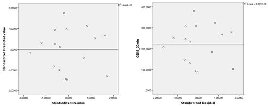
Figure 6.
Compliance of homoscedasticity of residuals. D3 building.
The scatter plot is a totally random point cloud, which shows neither trends nor patterns in the graphical representation. Consequently, the hypothesis of linearity and homoscedasticity is accepted.
For building D1, the supposed lack of multiple collinearity in the independent variable was also tested in the multiple linear regression model, represented by the Equation (6):
kWhD1 = 271,370.906 − 20,045.184 T_average + 50,568.513 V_night
This model corresponds to model 2, shown in Table 6.
Table 6.
Linear regression models. D1 building.
If two independent variables are closely correlated with each other and included in the model, certainly neither is likely to be statistically significant. However, if only one of them is included, it could prove to be statistically significant. To assess whether the model becomes unstable when a new variable is introduced, collinearity indices are evaluated. Following the studies of Belsley, Kuh, and Welsch, both with observed and simulated data, the problem of multicollinearity is severe when the condition index takes a value between 20 and 30 [53].
Table 7 shows the condition index for model 2, which is multiple linear regression, is 12.192, below 20. In addition, the tolerance shown in Table 6 takes a value of 0.738, close to the unit (the higher the tolerance, the lower the collinearity), so that it can be deduced that there is no multiple collinearity between the two independent variables.
Table 7.
Verification of the assumption of lack of multicollinearity between variables. D1 building.
2.5. Prediction of Expected Consumption
For the periods following construction of the network, using regression models and climate variables for subsequent periods, consumption without the district heating was predicted, and the accumulated consumption was calculated. This consumption was compared to the actual accumulated consumption. Table 8 shows the current consumption of building D3, corresponding to the period of the district heating from November 2015 to May 2017 and the values foreseen for the same period using the linear regression equation shown in Table 3.
Table 8.
Current and predicted consumption for building D3, from November 2015 to May 2017.
It can be seen in Table 8 and Figure 7 how the 15-month average of the actual consumption is 31,969 kWh during the two seasons following the installation of the district heating, while the 15-month average of expected consumption for these seasons if installation had not been built, was 35,307 kWh, 3338 kWh higher than actual consumption, representing a saving of 9.5%. However, as will be seen below, the priority saving is in fact not statistically significant.

Figure 7.
Mean real values and mean predicted values of consumption D3 building.
2.6. Statistical Verification of Significant Differences
An analysis was carried out to ascertain whether the difference between the predicted consumption, had the network not been built, and the actual consumption after it had been built, was statistically significant, at a confidence level of 95%.
The t-Student test was used in the study for related samples, which is considered particularly suited to compare the means of two groups when there is some relation between the individuals in the two groups. In this study, the relation was that consumption was associated to the same facility but during different periods of time.
Therefore, if the variables are distributed normally and the statistical significance is 0.05, it can be said that there are some significant differences. On the contrary, the null hypothesis that the two means are equal is not rejected, and the differences found are not considered statistically significant and do not go beyond what could be expected at random [54]. All of this assumes accepting a 5% error risk or, put differently, a confidence level of 95%.
The following shows how the differences found between the actual and predicted consumption of building D3 are not significant.
In line with the Shapiro–Wilk normality test, (Table 9) both the variables that represent actual consumption and those representing predicted consumption are distributed according to a normal distribution as a result of Sig. > 0.05, such that the null hypothesis of normality is accepted.
Table 9.
Test of normality for real and predicted consumption D3 building.
Table 10 shows that the forecast average consumption is 35,308 kWh, which compares with the actual average consumption of 31,969 kWh, which may lead one to believe that there is a difference of 3338 kWh between the averages.
Table 10.
Actual and predicted average consumption D3 building.
Table 11 shows that the difference found is not significant (value of Sig. > 0.05), such that we accept the null hypothesis of equal means. However, we are not in a position to say whether or not the difference found is due to more than mere chance.
Table 11.
Paired samples test D3 building.
2.7. Exploring the Possible Causes to Explain the Results Obtained
As a final step in the study, an analysis was carried out of the possible causes that might justify the statistical results of the existence or other wise of significant differences before and after the district heating works.
3. Results
The regression models found, which allow the consumption of each building to be explained in terms of the explanatory independent variables, are shown in Table 12. For building D1 (Apartments), a multiple regression model was found that predicted expected consumption with greater correlation. Table 12 includes the independent terms and the slopes of the regression variables (β), the Pearson linear correlation coefficients (R), and the linear determination coefficients between the variables (R2).
Table 12.
Regression models.
In seven of the 12 buildings, in other words 58.3% of the campus buildings, the explanatory variable found was degree-day on a 15 °C basis; the remaining 41.7% correlated better with mean temperature, and in building D1, in the regression multiple model, a new variable is introduced: nocturnal wind speed.
The absolute correlation value between the independent variables was between 0.896 and 0.999, and was positive for the models explained with the grade-day variable on a basis of 15 °C and negative for the mean temperature variables. The determination coefficient was between 0.802 and 0.998, so, accepting a risk error of 5%, the models found a predicted expected consumption with an accuracy probability greater than 80%., Figure 8 shows the linear regression model for building D3 (CTTA), displaying the consumption in kWh of the study period when the district heating was operating, and the straight line of consumption obtained with the explanatory variable.
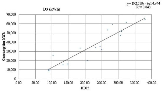
Figure 8.
Linear regression model. D3 building (Centre for the Transfer of Applied Technologies (CTTA)).
From the baselines of the regression models found and the climatic variables for the 2015–2017 periods, the expected or predicted consumption was obtained and compared with the actual consumption obtained in those periods. Figure 9 shows the results of actual consumption and forecast consumption (dashed line) for the periods following the installation of the district heating in several of the buildings on the Miguel Delibes campus. Building D3 (CTTA), where hardly any variation is observed, building D5 (University Institute of Applied Ophthalmology (IOBA)), where an increase in real consumption is observed with respect to the forecast, and building D1 (Apartments), where energy savings are observed.
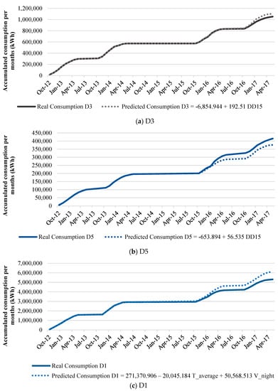
Figure 9.
Graphs of real and predicted consumption. D3, D5 and D1 buildings.
The differences found for each building and each of the facilities are shown in Table 13 and Table 14. The differences that turned out to be statistically significant are shaded. The savings that appear as negative are the increases in consumption.
Table 13.
Simple linear regression model.
Table 14.
Multiple regression model.
The significant savings differences in the simple linear regression analysis appear in buildings D1 (Apartments), D2 (Apartment Library), D4 (Teaching Block Library) and D12 (Research and Development (R&D) building), obtaining average savings of 21.3% (20.0% in D1, 30.6% in D2, 15.7% in D4, and 18.9% in D12). When applying the multiple regression model to the D1 building, significant savings in consumption continue to emerge, going from 20% in the simple model to 24.8% in the multiple model.
In two buildings: D5 (IOBA) and D8 (Building of Fine Chemistry and Advanced Materials (QUIFIMA)), statistically significant increases in consumption are observed; 16.1% for the 2016 season and 2017 in D5 and 23% for D8, although only in the 2017 season, reflecting an average increase in consumption of 20% for these buildings.
For the other six buildings, the differences found are not statistically significant.
Buildings D1, D2, D4 and D12 are buildings that are not used for teaching, so the time of use is extended to seven days a week and even to holiday periods in some cases.
4. Discussion
All the buildings studied used natural gas boilers as an initial system and in 50% of them no statistically significant differences were found between consumption before and after the installation of the heating network. Although this analysis did not reveal significant energy savings in all buildings, what is undeniable are the economic savings and emission savings achieved by substituting natural gas by biomass. This study analyses the viability of district heating in terms of predicting the expected heat demand, using as independent variables only the climatic data of the moment, and with a risk error equal to or less than 5%.
The results for the two heating seasons obtained to develop the baseline models (16 months) indicate that the regression mainly uses degree-days (58.3%) and mean temperature (41.7%) to establish its model, without taking into consideration the remaining variables such as: relative humidity, radiation, rainfall or wind speed. According to Granderson [55], a reference period of over 12 months does not guarantee a lower error.
The appropriateness of using district heating could be discussed depending on the initial system in operation to meet demand. As reflected in Ulseth’s work [56], this information is important in order to plan a district and conducting the financial feasibility study without making too many mistakes. In Norway, the use of heating networks to heat houses with heat pumps that were also used to meet the demand for domestic hot water was questioned. Other studies have even assessed the feasibility of using electricity as a source for a municipal district heating system with low local emissions, although this would clearly not be economically feasible given the current price of electricity [57].
The next step being taken in the UVA network is the use of solar thermal energy for domestic hot water (DHW), as Winterscheid presented in his studies [58]. This would certainly improve the energy efficiency of the grid and would also be the logical step for the gradual conversion to a fourth generation grid, as Pavicevic explained in his work on a district heating system in Zagreb [59].
Given the layout of university and regional administration buildings that are close to the grid, but not yet connected, and that there are heating systems with different thermal jumps, new buildings can be cascaded, rather than parallel, as in the case of the proposal presented by Mertz [60]. Buildings that require lower temperatures (buildings with all-air systems) could be connected to the exit of buildings that require higher temperatures (hospitals or clinics).
5. Conclusions
The case study provides an example of how district heating by biomass can improve a city’s environmental performance. The level of energy efficiency can still clearly be improved, since the savings obtained to date in the district heating system of the Miguel Delibes campus, where 12 buildings have been evaluated, is higher than 21% in 33% of the buildings. Overall, the district heating has achieved a significant reduction in CO2 emissions (6800 tons of CO2) according to the UVA, having changed natural gas for biomass (wood chips), also obtaining a significant economic saving of more than 30%.
The UVA district heating has achieved a reduction in installed power, going from 59 natural gas boilers with a total installed power of 27.4 MW to three boilers of 4.7 MW each, representing a total power of 14.1 MW.
A consumption model has been obtained for the Miguel Delibes university campus, which consists of 12 buildings and has an initial installed power of 9 MW, with a risk of error of 5%, and which has exceeded all statistical requirements to validate this type of model.
The response variable used to generate the models was natural gas consumption data for the 12 buildings from October 2012 to May 2014 and the climatic conditions in the area were used as an explanatory variable.
In 58% of the buildings, the variable that best correlates in the model found for the baseline was the grade-day, while for the remaining 42% it was the mean temperature. Variables such as relative humidity, rain, radiation or wind speed were not significant in the simple linear regression models found.
The absolute value of the correlation between the independent variables was between 0.896 and 0.99, and was positive for the models with the base explanatory variable of 15 degree-days and negative for the models with the mean temperature explanatory variable.
For 33% of the campus buildings, the savings obtained to date with this third generation is significant and above the 21% average. For 17% of the campus buildings, there is a significant increase in consumption, with an estimated average of around 20%. For the remaining 50% of the buildings, no significant differences were found in consumption before and after the installation of district heating.
Author Contributions
J.F.S.J.A. and F.J.R.M. conceived and designed the experiments; A.M.M.D. performed the experiment and analyzed the data; J.M.R.-H. wrote the paper and R.M.C. contributed simulation tools.
Funding
This research received no external funding.
Acknowledgments
The work presented in this article has been made possible thanks to the support of the University of Valladolid (UVA), the cooperation of the Public Infrastructures and Environment Company at the Regional Government of Castilla y León (SOMACYL), Institute of Advanced Production Technologies (ITAP) and RETO GIRTER Project (New Intelligent Manager for Thermal Networks), project funded by the European Regional Development Fund through the “2016 RETOS COLABORACIÓN” Program of the Ministry of Economy, Industry and Competitiveness of the Government of Spain.
Conflicts of Interest
The authors declare no conflict of interest.
References
- International Energy Agency (IEA). Market Report Series: Energy Efficiency 2017. Analysis and Forecasts to 2022; IEA: Paris, France, 2017. [Google Scholar]
- Communication from the Commission to the European Parliament, the Council, the European Economic and Social Committee and the Committee of the Regions. Energy Roadmap 2050. Available online: https://eur-lex.europa.eu/legal-content/EN/TXT/?uri=celex%3A52007DC0575 (accessed on 18 October 2018).
- IPCC. Climate Change 2014: Synthesis Report. Contribution of Working Groups I, II and III to the Fifth Assessment Report of the Intergovernmental Panel on Climate Change. Available online: http://www.ipcc.ch/pdf/assessment-report/ar5/syr/SYR_AR5_FINAL_full_wcover.pdf (accessed on 18 October 2018).
- Effort Sharing Regulation, 2021–2030. Limiting Member States’ Carbon Emissions; European Parliament: Bruxelles, Belgium. Available online: http://www.europarl.europa.eu/thinktank/en/document.html?reference=EPRS_BRI(2016)589799 (accessed on 18 October 2018).
- Ministerio de Fomento, Gobierno de España. Actualización De la Estrategia a Largo Plazo para la Rehabilitación Energética en el Sector de la Edificación en España (ERESEE 2017); Ministerio de Fomento: Madrid, Spain, 2017.
- IDAE. PROYECTO SECH-SPAHOUSEC Análisis del Consumo Energético del Sector Residencial en España; IDAE: Madrid, Spain, 2011. [Google Scholar]
- Directive 2009/28/EC of the European Parliament and of the Council of 23 April 2009 on the Promotion of the Use of Energy from Renewable Sources and Amending and Subsequently Repealing Directives 2001/77/EC and 2003/30/EC. Available online: http://data.europa.eu/eli/dir/2009/28/oj (accessed on 18 October 2018).
- United Nations Environment Programme (UNEP). District Energy in Cities: Unlocking the Potential of Energy Efficiency and Renewable Energy. Available online: http://hdl.handle.net/20.500.11822/9317 (accessed on 18 October 2018).
- The European Parliament and the Council of the European Union DIRECTIVE (EU) 2018/844 of the European Parliament and of the Council of 30 May 2018 Amending Directive 2010/31/EU on the Energy Performance of Buildings and Directive 2012/27/EU on Energy Efficiency. Off. J. Eur. Union 2018. Available online: https://eur-lex.europa.eu/legal-content/EN/TXT/PDF/?uri=CELEX:32018L0844&from=IT (accessed on 18 October 2018).
- Van Deventer, J.; Derhamy, H.; Atta, K.; Delsing, J. Service Oriented Architecture enabling the 4th Generation of District Heating. Energy Procedia 2017, 116, 500–509. [Google Scholar] [CrossRef]
- Lee, J.S.; Kim, H.C.; Im, S.Y. Comparative Analysis between District Heating and Geothermal Heat Pump System. Energy Procedia 2017, 116, 403–406. [Google Scholar] [CrossRef]
- Ericsson, K.; Werner, S. The introduction and expansion of biomass use in Swedish district heating systems. Biomass Bioenergy 2016, 94, 57–65. [Google Scholar] [CrossRef]
- Sandvall, A.F.; Ahlgren, E.O.; Ekvall, T. Cost-efficiency of urban heating strategies—Modelling scale effects of low-energy building heat supply. Energy Strateg. Rev. 2017, 18, 212–223. [Google Scholar] [CrossRef]
- Lund, H.; Möller, B.; Mathiesen, B.V.; Dyrelund, A. The role of district heating in future renewable energy systems. Energy 2010, 35, 1381–1390. [Google Scholar] [CrossRef]
- Delmastro, C.; Mutani, G.; Schranz, L. Advantages of Coupling a Woody Biomass Cogeneration Plant with a District Heating Network for a Sustainable Built Environment: A Case Study in Luserna San Giovanni (Torino, Italy). Energy Procedia 2015, 78, 794–799. [Google Scholar] [CrossRef]
- Wojdyga, K.; Chorzelski, M. Chances for Polish district heating systems. Energy Procedia 2017, 116, 106–118. [Google Scholar] [CrossRef]
- Kolokotsa, D. The role of smart grids in the building sector. Energy Build. 2016, 116, 703–708. [Google Scholar] [CrossRef]
- Laakkonen, L.; Korpela, T.; Kaivosoja, J.; Vilkko, M.; Majanne, Y.; Nurmoranta, M. Predictive Supply Temperature Optimization of District Heating Networks Using Delay Distributions. Energy Procedia 2017, 116, 297–309. [Google Scholar] [CrossRef]
- Bush, R.E.; Bale, C.S.E. The role of intermediaries in the transition to district heating. Energy Procedia 2017, 116, 490–499. [Google Scholar] [CrossRef]
- Ziemele, J.; Gravelsins, A.; Blumberga, A.; Blumberga, D. The Effect of Energy Efficiency Improvements on the Development of 4th Generation District Heating. Energy Procedia 2016, 95, 522–527. [Google Scholar] [CrossRef]
- Lake, A.; Rezaie, B.; Beyerlein, S. Review of district heating and cooling systems for a sustainable future. Renew. Sustain. Energy Rev. 2017, 67, 417–425. [Google Scholar] [CrossRef]
- Werner, S. District heating and cooling in Sweden. Energy 2017, 126, 419–429. [Google Scholar] [CrossRef]
- Wouters, C. Towards a regulatory framework for microgrids—The Singapore experience. Sustain. Cities Soc. 2015, 15, 22–32. [Google Scholar] [CrossRef]
- Schmidt, D.; Kallert, A.; Blesl, M.; Svendsen, S.; Li, H.; Nord, N.; Sipilä, K. Low Temperature District Heating for Future Energy Systems. Energy Procedia 2017, 116, 26–38. [Google Scholar] [CrossRef]
- Averfalk, H.; Werner, S. Essential improvements in future district heating systems. Energy Procedia 2017, 116, 217–225. [Google Scholar] [CrossRef]
- Rämä, M.; Sipilä, K. Transition to low temperature distribution in existing systems. Energy Procedia 2017, 116, 58–68. [Google Scholar] [CrossRef]
- Wahlroos, M.; Pärssinen, M.; Manner, J.; Syri, S. Utilizing data center waste heat in district heating—Impacts on energy efficiency and prospects for low-temperature district heating networks. Energy 2017, 140, 1228–1238. [Google Scholar] [CrossRef]
- Persson, U.; Münster, M. Current and future prospects for heat recovery from waste in European district heating systems: A literature and data review. Energy 2016, 110, 116–128. [Google Scholar] [CrossRef]
- Nord, N.; Schmidt, D.; Kallert, A.M.D. Necessary Measures to Include more Distributed Renewable Energy Sources into District Heating System. Energy Procedia 2017, 116, 48–57. [Google Scholar] [CrossRef]
- Flores, J.F.C.; Lacarrière, B.; Chiu, J.N.W.; Martin, V. Assessing the techno-economic impact of low-temperature subnets in conventional district heating networks. Energy Procedia 2017, 116, 260–272. [Google Scholar] [CrossRef]
- Lund, H.; Werner, S.; Wiltshire, R.; Svendsen, S.; Thorsen, J.E.; Hvelplund, F.; Mathiesen, B.V. 4th Generation District Heating (4GDH): Integrating smart thermal grids into future sustainable energy systems. Energy 2014, 68, 1–11. [Google Scholar] [CrossRef]
- Council Directive 2010/31/EU of 19 May 2010 on the Energy Performance of Buildings, in 2010 OJ L153/13. Available online: http://data.europa.eu/eli/dir/2010/31/oj (accessed on 18 October 2018).
- Directive 2012/27/EU of the European Parliament and of the Council of 25 October 2012 on Energy Efficiency, Amending Directives 2009/125/EC and 2010/30/EU and Repealing Directives 2004/8/EC and 2006/32/EC. Available online: http://data.europa.eu/eli/dir/2012/27/oj (accessed on 18 October 2018).
- Communication From the Commission to the European Parliament, the Council, the European Economic and Social Committee and the Committee Of The Regions, an EU Strategy on Heating and Cooling. COM/2016/051 Final. Available online: https://eur-lex.europa.eu/legal-content/en/TXT/?uri=CELEX%3A52016DC0051 (accessed on 18 October 2018).
- Werner, S. International review of district heating and cooling. Energy 2017, 137, 617–631. [Google Scholar] [CrossRef]
- Sathaye, J.; Murtishaw, S.; Price, L.; Lefranc, M.; Roy, J.; Winkler, H.; Spalding-Fecher, R. Multiproject baselines for evaluation of electric power projects. Energy Policy 2004, 32, 1303–1317. [Google Scholar] [CrossRef]
- UNE-EN ISO 15927-6:2009. Hygrothermal Performance of Buildings—Calculation and Presentation of Climatic Data—Part 6: Accumulated Temperature Differences (Degree-Days) (ISO 15927-6:2007). Available online: https://www.une.org/encuentra-tu-norma/busca-tu-norma/norma/?c=N0043434 (accessed on 18 October 2018).
- Golden, A.; Woodbury, K.; Carpenter, J.; O’Neill, Z. Change point and degree day baseline regression models in industrial facilities. Energy Build. 2017, 144, 30–41. [Google Scholar] [CrossRef]
- Meng, Q.; Mourshed, M. Degree-day based non-domestic building energy analytics and modelling should use building and type specific base temperatures. Energy Build. 2017, 155, 260–268. [Google Scholar] [CrossRef]
- Verbai, Z.; Lakatos, Á.; Kalmár, F. Prediction of energy demand for heating of residential buildings using variable degree day. Energy 2014, 76, 780–787. [Google Scholar] [CrossRef]
- Atalla, T.; Gualdi, S.; Lanza, A. A global degree days database for energy-related applications. Energy 2018, 143, 1048–1055. [Google Scholar] [CrossRef]
- De Rosa, M.; Bianco, V.; Scarpa, F.; Tagliafico, L.A. Heating and cooling building energy demand evaluation; A simplified model and a modified degree days approach. Appl. Energy 2014, 128, 217–229. [Google Scholar] [CrossRef]
- Efficiency Valuation Organization (EVO). International Performance Measurement and Verification Protocol: Concepts and Options for Determining. 2010. Available online: https://evo-world.org/en/products-services-mainmenu-en/protocols/ipmvp (accessed on 18 October 2018).
- IBM SPSS Software. Available online: https://www.ibm.com/analytics/spss-statistics-software (accessed on 15 September 2018).
- Walpole, R.E.; Myers, R.H.; Myers, S.L. Probabilidad y Estadística Para Ingeniería y Ciencias, 9th ed.; Prentice Hall: Englewood Cliffs, NJ, USA, 2012; ISBN 9786073214179. [Google Scholar]
- Bilous, I.; Deshko, V.; Sukhodub, I. Parametric analysis of external and internal factors influence on building energy performance using non-linear multivariate regression models. J. Build. Eng. 2018, 20, 327–336. [Google Scholar] [CrossRef]
- Permai, S.D.; Tanty, H. Linear regression model using bayesian approach for energy performance of residential building. Procedia Comput. Sci. 2018, 135, 671–677. [Google Scholar] [CrossRef]
- Roth, J.; Rajagopal, R. Benchmarking building energy efficiency using quantile regression. Energy 2018, 152, 866–876. [Google Scholar] [CrossRef]
- Fumo, N.; Rafe Biswas, M.A. Regression analysis for prediction of residential energy consumption. Renew. Sustain. Energy Rev. 2015, 47, 332–343. [Google Scholar] [CrossRef]
- Arregi, B.; Garay, R. Regression analysis of the energy consumption of tertiary buildings. Energy Procedia 2017, 122, 9–14. [Google Scholar] [CrossRef]
- Aranda, A.; Ferreira, G.; Mainar-Toledo, M.D.; Scarpellini, S.; Llera Sastresa, E. Multiple regression models to predict the annual energy consumption in the Spanish banking sector. Energy Build. 2012, 49, 380–387. [Google Scholar] [CrossRef]
- Savin, N.E.; White, K.J. The Durbin-Watson test for serial correlation with extreme sample sizes or many regressors. Econom. J. Econom. Soc. 1977, 1989–1996. [Google Scholar] [CrossRef]
- Belsley, D.A.; Kuh, K.; Welsch, R.E. Regression Diagnostics: Identifying Influential Data and Sources of Collinearity; John Wiley & Sons: New York, NY, USA, 1980; ISBN 0-471-05856-4. [Google Scholar]
- Navidi, W. Estadística Para Ingenieros y Científicos; McGraw-Hill: New York, NY, USA, 2006; ISBN 970-10-5629-9. [Google Scholar]
- Granderson, J.; Price, P.N. Development and application of a statistical methodology to evaluate the predictive accuracy of building energy baseline models. Energy 2014, 66, 981–990. [Google Scholar] [CrossRef]
- Lindberg, K.B.; Georges, L.; Alonso, M.J.; Utne, Å. Measured load profiles and heat use for “low energy buildings” with heat supply from district heating. Energy Procedia 2017, 116, 180–190. [Google Scholar] [CrossRef]
- Khabdullin, A.; Khabdullina, Z.; Khabdullina, G.; Lauka, D.; Blumberga, D. Demand response analysis methodology in district heating system. Energy Procedia 2017, 128, 539–543. [Google Scholar] [CrossRef]
- Winterscheid, C.; Dalenbäck, J.-O.; Holler, S. Integration of solar thermal systems in existing district heating systems. Energy 2017, 137, 579–585. [Google Scholar] [CrossRef]
- Pavičević, M.; Novosel, T.; Pukšec, T.; Duić, N. Hourly optimization and sizing of district heating systems considering building refurbishment—Case study for the city of Zagreb. Energy 2017, 137, 1264–1276. [Google Scholar] [CrossRef]
- Mertz, T.; Serra, S.; Henon, A.; Reneaume, J.M. A MINLP optimization of the configuration and the design of a district heating network: study case on an existing site. Energy Procedia 2017, 116, 236–248. [Google Scholar] [CrossRef]
© 2018 by the authors. Licensee MDPI, Basel, Switzerland. This article is an open access article distributed under the terms and conditions of the Creative Commons Attribution (CC BY) license (http://creativecommons.org/licenses/by/4.0/).