Abstract
The corrosion diagnosis of grounding grid can locate the corroded branches and provide guidance for the maintenance and repair of the grounding grid. This paper proposed the electrical impedance tomography (EIT) method on the corrosion diagnosis of grounding grid and described how it works. Firstly, the inverse problem model of the electrical impedance tomography on grounding grid is developed. Secondly, in order to weaken the ill-posedness of the inverse problem, a Newton iterative algorithm with Tikhonov regularization is proposed to solve the problem. Then, due to the high resistivity contrast between the soli and steel and the large size of imaging region, this paper presents the method of soil-separation and block-diagnosis to accomplish these problems. Finally, field experiments were carried out to verify the effectiveness of the proposed method and the results show that the location and degree of the corrosion in the grounding grid can be easily judged from the imaging results.
1. Introduction
Grounding grid is an important part of electrical power system at substation for the discharge of dangerous current and safety of persons working at substation [1]. Grounding grid is vulnerable to corrosion due to working in moist underground environment for long time, which will weaken its ability of current-dispersing and voltage-sharing. Therefore, corrosion diagnosis on the grounding grid to locate the corrosion branch is essential to make some prevention and maintenance measures timely.
In China and some other developing countries, the grounding grid is usually made up of steel, so the corrosion state is more severe. Research on the grounding grid has received more attention in recent years. From the previous literatures, some of them focused on the optimal design and the safety performance analysis of the grounding grid [2,3,4,5,6] and others pay more attention to the corrosion diagnosis. As the grounding grid is buried under the ground, it is difficult to detect the corrosion directly. Therefore, some researchers devoted themselves on the corrosion diagnosis of the grounding grid with some non-contact methods. So far, the diagnosis methods mainly based on the electric network theory and electromagnetic field. The electric network theory method makes the grounding grid an equivalent resistor network and measures the potentials or the port resistance of the down-lead lines to calculate the branch resistance and then determine the corrosion state of grounding grid by comparing the value calculated with the initial design resistance of the grounding grid [7,8,9]. In the study so far, the diagnosis method based on electric network theory simply regard the branch as a resistor but do not consider the distributed parameter of the grounding grid, for example the resistivity, so this method can only locate which branch is eroded but cannot know the accurate corrosion point in the branch. On the other hand, the down-lead lines are not in the branch intersection nodes will have a great effect on the accuracy of the electrical network method. The method based on electromagnetic field through measuring and analyzing the surface magnetic field [10] or the transient magnetic field of grounding grid to judge the corrosion state of the grounding grid [11,12]. In addition, Liu et al. [13] utilized the magnetic field above the grounding grid to reconstruct the resistivity distribution image to find the break-point of the branch. While, electromagnetic field methods can judge the break-point but insensitive to the corrosion and the electromagnetic environment in the substation is complicated, the measurements of magnetic data are vulnerable to the noise and usually inaccurate. Hence, it is very important and urgent to find another effective method to do the grounding grid corrosion diagnosis.
In this paper, a diagnosis method based on electrical impedance tomography is put forward. EIT is a noninvasive, inexpensive new imaging technology and it is normally applied in the medical field [14,15,16]. Due to the different resistivity between the corroded and the normal steel, the corrosion diagnosis of the grounding grid is potentially feasible through the resistivity distribution image obtained by EIT. Similar to the medical EIT, the grounding grid EIT implemented by injecting a current into the grounding grid and measuring the potentials of the down-lead lines and then use the data to reconstruct the resistivity distribution image. Based on the topology of grounding grid obtained by derivative method [17] or wavelet edge detection [18], we proposed soil-separation and block-diagnosis methods to improve the diagnosis accuracy. Simulations and field experiment are carried out and the results show the corrosion degree and corrosion location in the branch of grounding grid can be achieved correctly.
2. Model and Algorithm
This section gives the model and algorithm of grounding grid EIT, including the comparison of physical model between the medical EIT and the grounding grid EIT and the mathematical reconstruction algorithm.
2.1. The Physical Model
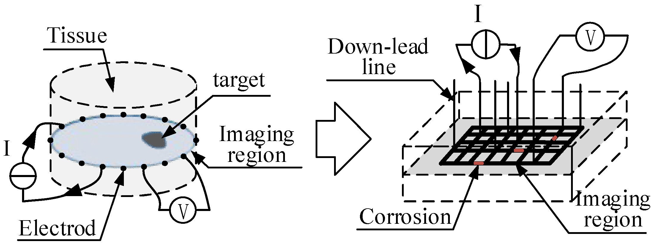
The medical EIT technology can attain the resistivity distribution of the imaging region through the boundary potentials and then the imaging result will provide some medical information for the clinic. For the grounding grid, when the grounding grid branch is corroded, the resistivity of the corrosion will be higher than the normal steel. So, we can use EIT to locate the corrosion and judge the corrosion degree in the grounding grid.
Compared with the medical EIT, the EIT of the grounding grid is similar but different in a sense that for the medical EIT. In the medical EIT, the electrodes are on the boundary of the imaging region. However, in the grounding grid EIT, the grounding grid is buried underground, we make the down-lead lines as the electrodes to inject current and measure potentials. The down-lead lines are not on the boundary but in the region, so we call it inner-source EIT or improved EIT. On the other hand, the imaging region size of the grounding grid is much bigger than that of medical EIT and the differences in resistivity of soil and steel, we call it resistivity contrast, is great. In summary, a comparison of the field characteristics between the medical EIT and the grounding grid corrosion diagnosis is shown in Table 1.

Table 1.
Comparison between medical EIT and grounding grid EIT.
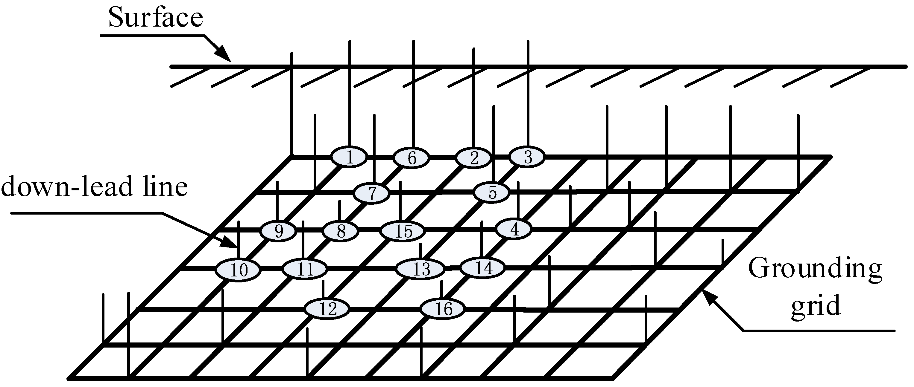
From the differences compared above, the physical model of medical EIT and simplified grounding grid EIT can be described in Figure 1 as follows.

Figure 1.
The physical model of medical EIT and grounding grid EIT.
2.2. The Forward Problem
The reconstruction algorithm of grounding grid EIT consists of forward problem and inverse problem. The forward problem of grounding grid EIT is to calculate the potentials of down-lead lines when the resistivity distribution of the grounding grid region is given and this process can be realized through the Finite Element Method (FEM) [19].
When injected a DC in the grounding grid, according to the electromagnetic field theory, the potential distribution can be expressed as:
where and are the conductivity and potential of grounding grid field respectively.
And the boundary conditions are
where f is potential of the boundary, is the boundary of , j is the current density injected into the , is the outer normal vector of the .
The forward problem (1)–(3) can be solved with finite element method (FEM), after meshing and functional analysis, it derives
where is the potentials of nodes and K is the coefficient matrix only related to coordinates and the resistivity of each element.
The boundary conditions for the (4) are applied as follows, assume that the inflow and outflow nodes of the current are respectively corresponding to the node m and node n of the finite element model and select the node l as the potential reference point, the injected current is I. Hence, we obtain
This is the FEM equation of the forward problem. By solving the (5), the potential of each node can be obtained, that is the solution to the forward problem.
2.3. The Inverse Problem
In the practical corrosion diagnosis of grounding grid, the resistivity distribution is unknown and we can only measure the injected current and the potentials on the down-lead lines. The goal of EIT is to reconstruct the resistivity distribution image by using these potentials and excitation current information, this process is opposite to the forward problem, so call it the inverse problem in the EIT.
In practice, it is almost impossible to obtain the exact solution of the inverse problem, namely, the exact solution does not exist or is difficult to find. In order to find an approximate solution with engineering significance, the least square solution is used to approximate the true solution of the inverse problem. Therefore, the inverse problem is built to find the resistivity distribution to minimize the error between the calculated potentials and the measured data [20]. The mathematical equation can be expressed as follows:
where is the calculated potential by the forward problem, is the measured potential, i and j is the measurement times and measurements in each time. The is a function of , we call it error function.
Formula (6) is a typical nonlinear optimal value problem and this paper uses the Newton iteration method to solve the problem, the iterative formula is derived as:
where is the Jacobi matrix of the node potential to the element resistivity. If the imaging region has u elements and n measurement potentials, the Jacobi matrix would be
As the amount of measured data is much less than the number of elements, the in (7) is a non-full rank matrix and its inverse matrix cannot be calculated directly, therefore the inverse problem is severely ill-posed.
In order to weaken the ill-posedness of the inverse problem, the Tikhonov regularization was applied to solve the inverse problem. It can solve the inverse problem stably through adding a penalty function to the objective function, the mathematical model is
where is the regularization parameter selected by L-curve method [21] and L is the regularization matrix (identity matrix in this method).
In the FEM model of EIT, the iterative formula of Newton iteration method with Tikhonov regularization can be derived from (9) as follows:
Through solving (10) with coding in the MATLAB (R2014a, Mathworks, Natick, MA, USA ), we can obtain the resistivity distribution and the image of the resistivity distribution can be achieved.
3. Corrosion Diagnosis Method
3.1. Potential Measurement
The excitation of grounding EIT is a DC source. In the potential measurement, to reduce the interference of power frequency leakage current in the grounding grid, we only extracting the DC component of the signal to filter the AC potential signal to reduce the noise. On the other hand, the amount of potentials on the down-lead lines is a significant factor affecting the imaging resolution (discussed in Section 4.2). In order to make full use of the down-lead lines to get information of the grounding grid, we use the cycle measurement [22] to get more node potentials. For example, for a grounding grid in Figure 2, the process of cycle measurement by using a 16-channel potential acquisition device is as follows: choose two down-lead lines arbitrarily from the 16 down-lead lines as the current inflow point and outflow point, according to the tetrapolar measurement method, choose another down-lead line as the potential reference point and then we can measure the potentials of the remaining 13 down-lead lines. Change the inflow and outflow point of the current circularly, we can obtain another 13 potentials. Through the cycle measurement, except the potential reference point and the current drive points, the amount of the potentials would be . The cycle measurement increased the amount of data as well as the measuring efficiency.
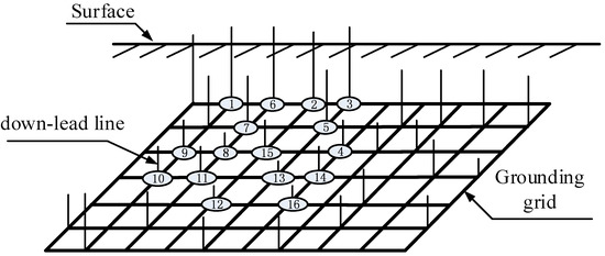
Figure 2.
The cycle measurement of potentials.
3.2. The Soil-Separation Method
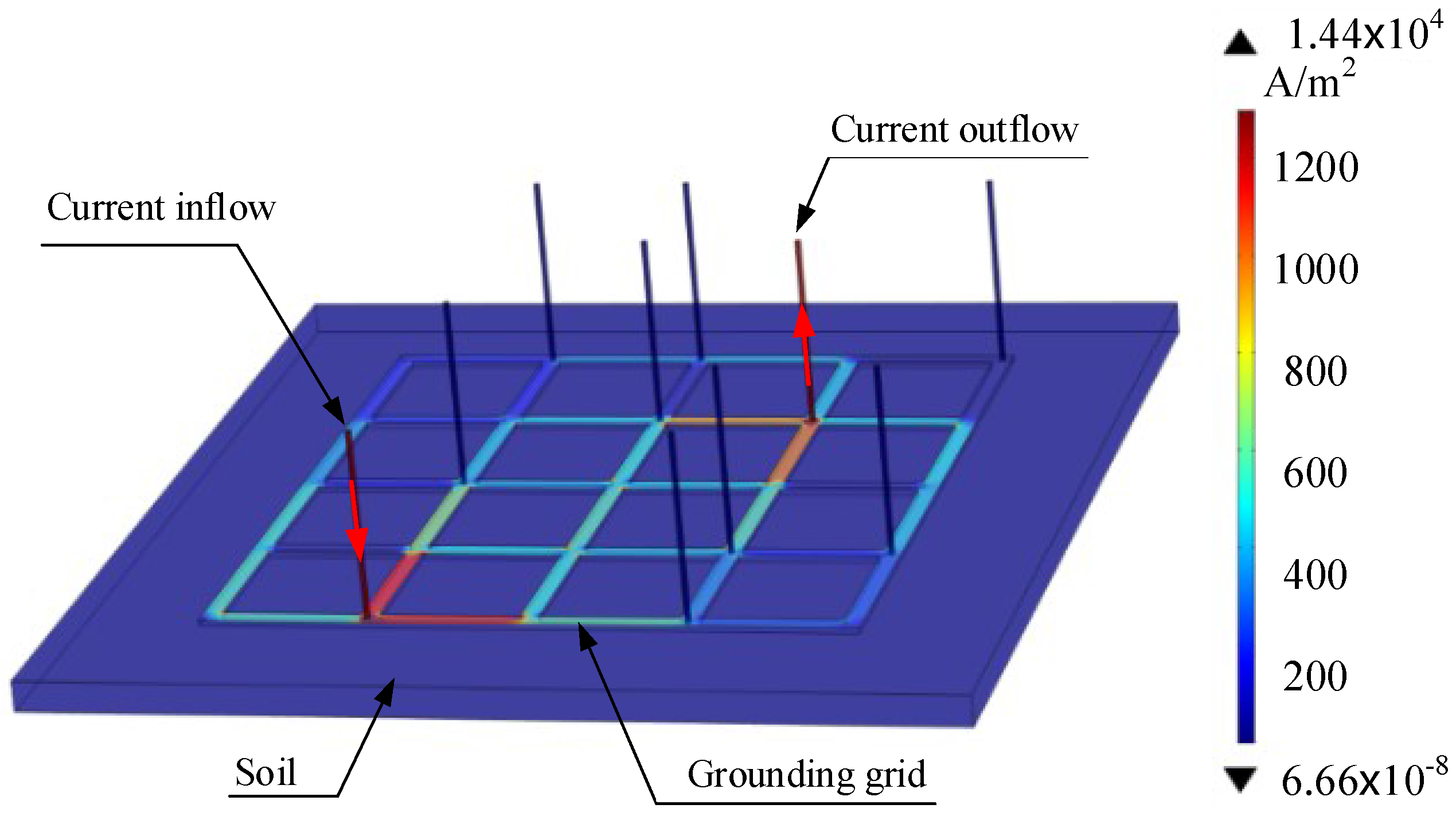
For the grounding grid field, the soil resistivity (about 102 ) and the resistivity of grounding grid (about 10−7 ) is high-contrast, hence the injected current is bounded into the branches. A simulation result in Figure 3 indicates this point. In the simulation model, we set the resistivity of the soil and the grounding grid is 102 and 10−7 respectively and the injected current is 1 A.

Figure 3.
The current density distribution of grid field.
From Figure 3, the current that flows through in the soil is extremely low. So, we can conclude that the soil is an ideal insulator when the injected current is not big and it is reasonable to ignore the soil when performing the EIT on the grounding grid field. Therefore, we only need to consider the grounding grid as the target region of imaging to improve the resolution.
As analyzed above, there is almost no current flows into the soil when the injected current is small. In addition, the objective of corrosion diagnosis on the grounding grid is to locate where the corroded steel is, so we do not pay attention to the soil. Due to the high contrast of the resistivity between the soil and the steel branches, in the grounding grid EIT, the potentials of the down-lead lines are extremely low-sensitive to the soil, which would increase the condition number of the Jacobi matrix and aggravate the ill-posedness of the inverse problem. Therefore, this paper proposes the method to separate the grounding grid from the soil and only perform the EIT on the grounding grid branch to improve the resolution of the resistivity distribution imaging.
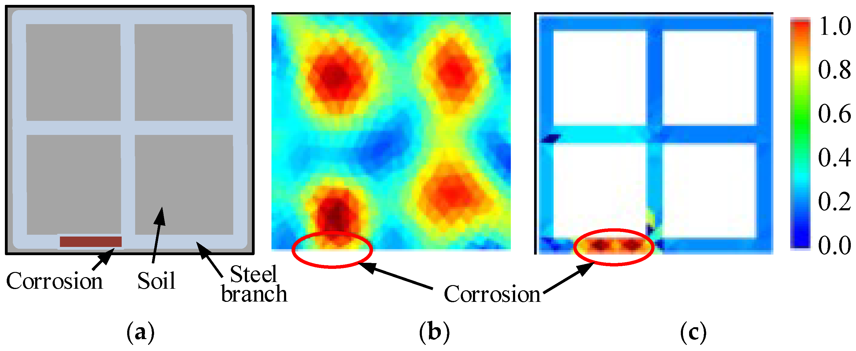
A simulation experiment on the grounding grid block was conducted to compare the EIT results of the soil-separation method with the method taking the soil into account. One corrosion fault was set in the branch, the mesh of FEM model and imaging results about the normalized resistivity distribution are shown in Figure 4 and Figure 5. From the results, the corrosion fault can be judged in both two images but the location and size of the corrosion in the image with the soil is not clear and its resolution is also lower than the image without soil.
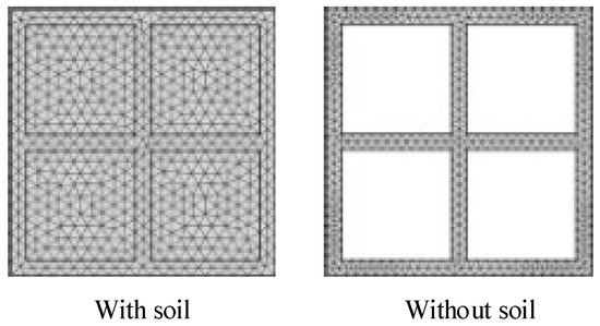
Figure 4.
The meshing results of the FEM model.

Figure 5.
Imaging results with and without soil. (a) Imaging model; (b) With soil; (c) Without soil.
3.3. The Block-Diagnosis Method
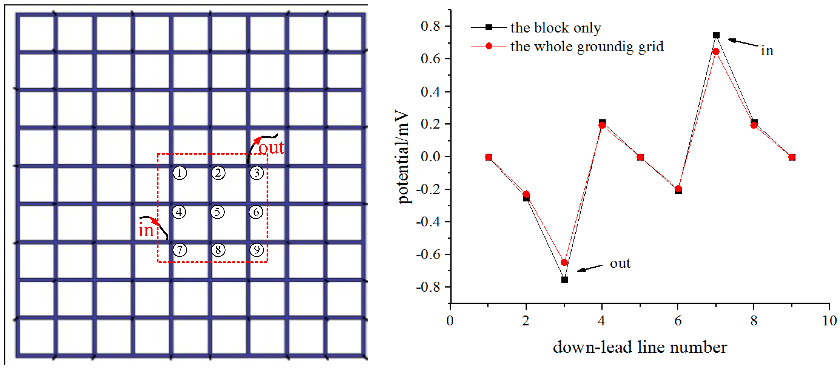
Due to the size of grounding grid region is very big, if we reconstruct the resistivity distribution in one image, which would worsen the resolution of the image as well as increase the computational cost. So, we divided the whole grounding grid into many basic blocks and performed the imaging of each block. Actually, we can only diagnose the grounding grid blocks under and near some important equipment to improve the diagnosis efficiency. While in a large grounding grid, when we injected a current into the block, shown in Figure 6, a part of the current will flow through the grounding grid outside the block. According to the principle of minimum energy in the electrical network, only a little current will flow outside the block, which will have a slight effect on the boundary potentials. To verify this point, in the forward problem solved by FEM, we compared the potentials on the down-lead lines of the block only and with considering the outside grounding grid. From the calculation results, there are relatively large errors on the current inflow and outflow points. In order to reduce the slight effect on the boundary potentials to improve the imaging accuracy, we remove the potentials on the current inflow and outflow down-lead lines in the inverse problem calculation process.

Figure 6.
The potentials calculation on the block only and the whole grounding grid. (a) The grounding grid model; (b) The calculation results.
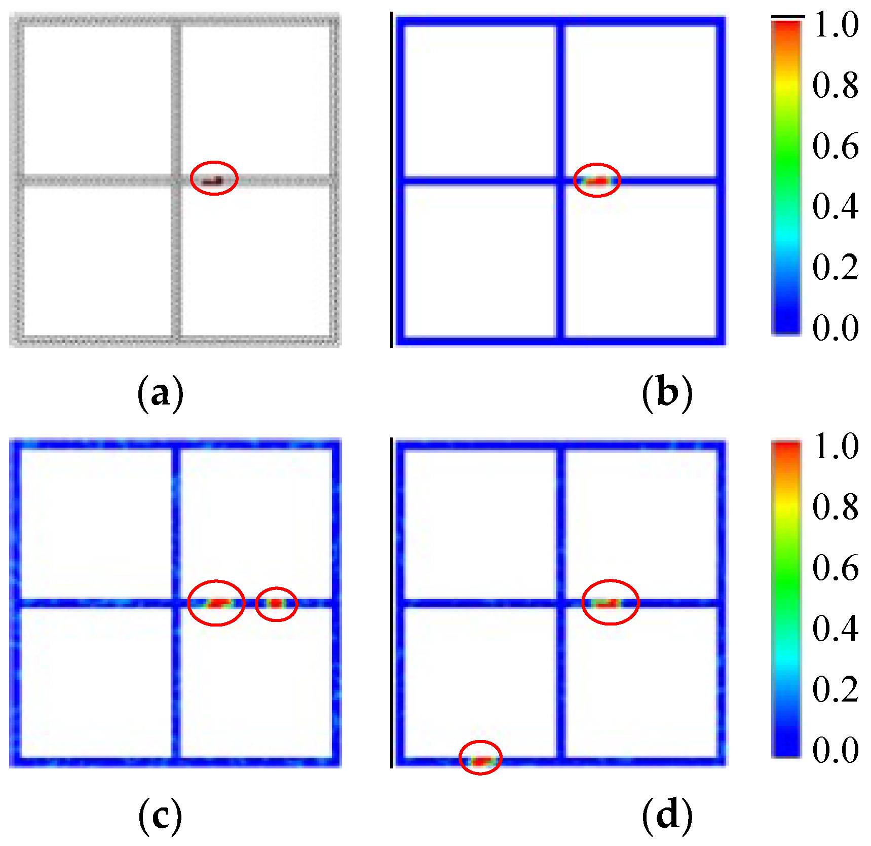
We used the simple block to do the block-diagnosis simulation, in the simulation experiments, the width of the steel is 5 cm and the resistivity contrast between the corrosion and the steel is set as 5:1 and the injected current is 1 A. Different corrosion faults in different branches are preset in the experiments. The corrosion diagnosis results about normalized resistivity distribution are shown in Figure 7.
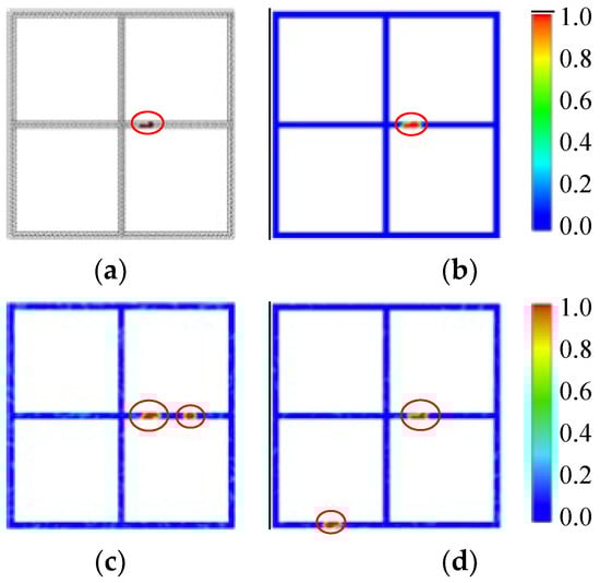
Figure 7.
The imaging result of corrosion diagnosis on block. (a) One corrosion fault setting; (b) One corrosion fault; (c) Two corrosion faults in one branch; (d) Two corrosion faults in two branches.
From the imaging results, no matter where the corrosion fault is, the location and size of the corrosion fault in the grounding gird are in a good agreement with the corrosion-setting.
4. Simulation Discussion
In order to cover different situations of the corroded grounding grid, we discuss different conditions or factors which may have influence on the EIT results. In the following discussion, the size of each grid of the grounding grid block is and the width of the steel is still 5 cm and the injected current is 1 A. In addition, all the imaging results are about the normalized resistivity distribution.
4.1. Different Shape of the Grounding Grid Block
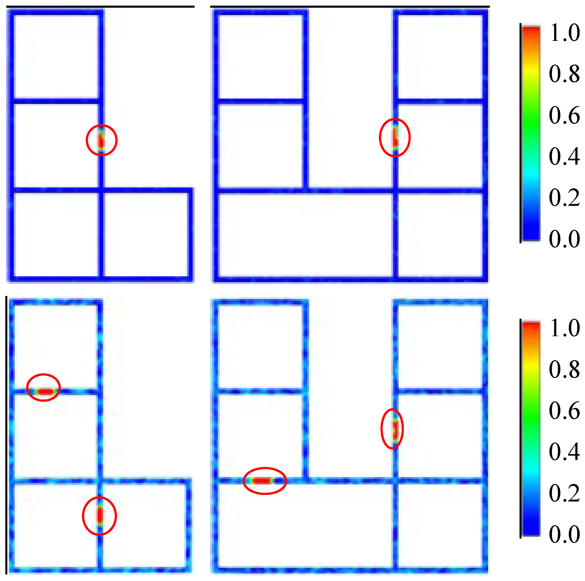
The grounding grid can not only be divided into many blocks but also some other different shapes. In order to consider more complex occasions, the same simulations were performed on the L-shape and U-shape grounding grid block, each block is set with one or two corrosion faults. Moreover, the resistivity contrast between the corrosion and the steel is set as 5:1. The Figure 8 describes imaging results as follows.

Figure 8.
The result of corrosion diagnosis on L-shape and U-shape block.
From the simulation results, it is found that the corrosion fault of the grounding grid can be accurately diagnosed by EIT and the image is straightforward to judge the location of the corrosion, which is not depended on the shape of the grounding grid block. Although there are some artefacts in the images for the two faults diagnosis, the result is still can locate the corrosion, it is significant for the engineering.
4.2. The Amount of the Measurements
According to the algorithm of the EIT, the elements in the FEM model are always more than the number of the potentials measurements, so the inverse problem is undetermined. When the amount of data is scarce, the imaging results maybe low-resolution, even cannot obtain a right imaging. We take a block for example to study the relationship between the amount of the measurements and the resolution of the image.
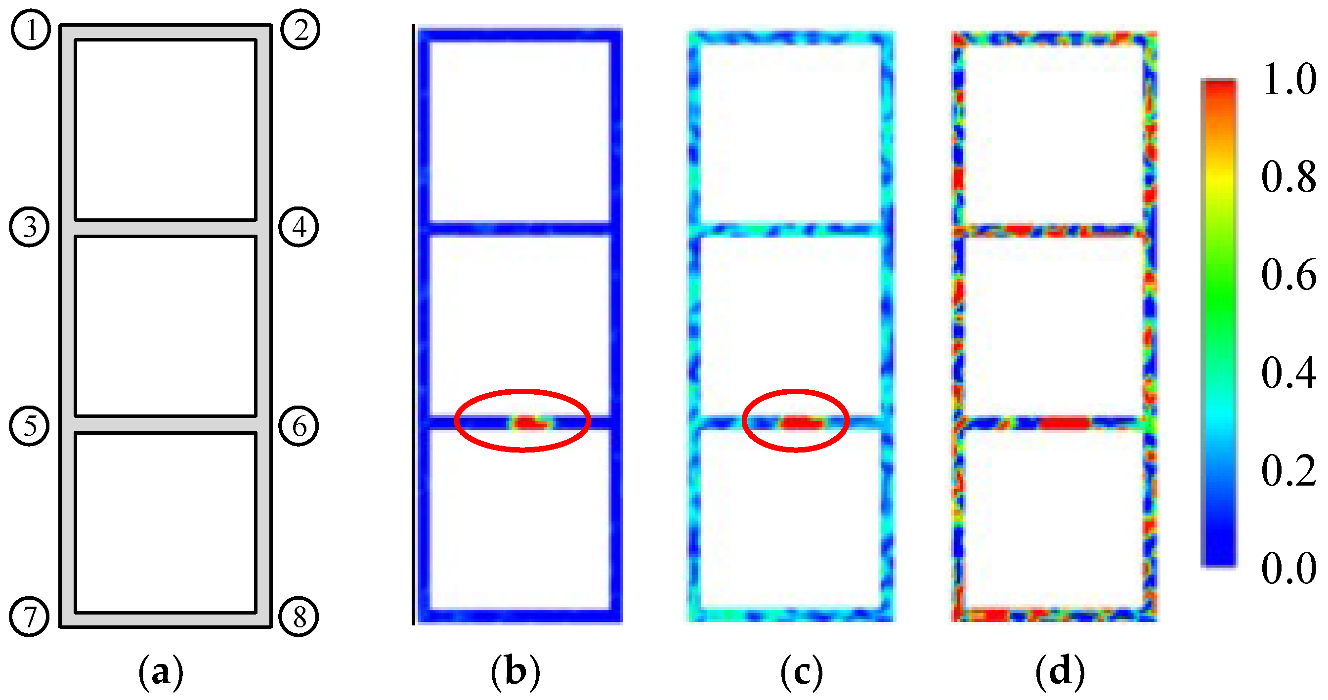
Assume there is one corrosion in the branch, whose resistivity is 5 times of the normal steel. The block has 8 nodes, we conducted three different imaging cases by using 8, 6, 4 nodes to acquire the potential data, the nodes chosen in each case is as follows
Case 1: 8 nodes are 1, 2, 3, 4, 5, 6, 7, 8;
Case 2: 6 nodes are 1, 2, 5, 6, 7, 8;
Case 3: 4 nodes are 1, 2, 7, 8.
According to the cycle measurement introduced in Section 3.1, the number of measurements in each case is 140, 45, 6. The corresponding imaging results are presented in Figure 9. Along with the decrease of measurements, the resolution of the image gets worse and it becomes difficult to judge the corrosion. When there are only 4 nodes for measuring the data, the resistivity distribution cannot be reconstructed successfully. Therefore, in the actual diagnosis, we should use cycle measurement and interpolation to get as more data as possible.

Figure 9.
The model and imaging results of block with different number of measurements. (a) Block model; (b) 8 nodes; (c) 6 nodes; (d) 4 nodes.
4.3. Different Corrosion Degrees
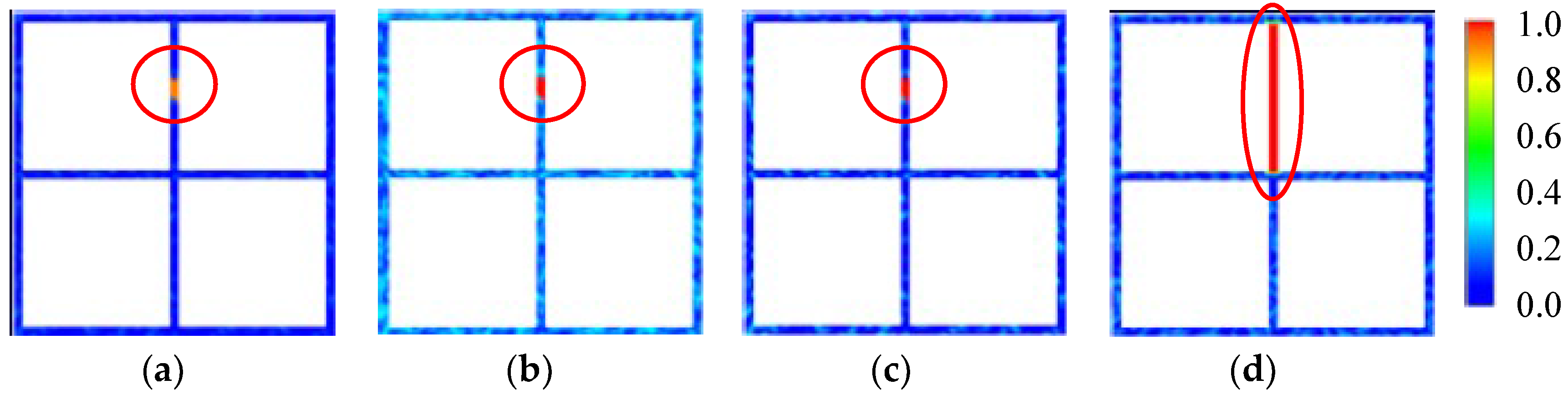
When the grounding grid is corroded severely, it will cause a break-point. To verify whether the imaging results can correctly reflect the different degrees of the corrosion, some simulation experiments were conducted. Through setting different resistivity contrast to simulate different corrosion degrees. Four cases are considered in the block as follows,
Case 1: one corrosion fault, the resistivity contrast is 3:1;
Case 2: one corrosion fault, the resistivity contrast is 10:1;
Case 3: one corrosion fault, the resistivity contrast is 50:1;
Case 4: one corrosion fault, the resistivity contrast is 106:1
The case 4 is to simulate the break-point.
The simulation results about the above cases are shown in Figure 10.
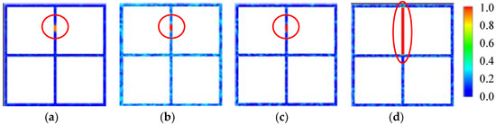
Figure 10.
The imaging results of block with different corrosion degrees. (a) Case 1; (b) Case 2; (c) Case 3; (d) Case 4.
In the resistivity distribution image obtained by the EIT, different shades of color reflected different degrees of corrosion, when the corrosion is becoming more serious, the red part in the image is becoming darker, which are agree with the different resistivity contrasts. When there is a break-point in the branch, the current will not flow in this branch, so the whole branch will be regarded as severe corrosion in the imaging result, just like the (d) in Figure 10.
5. Experimental Analysis
In order to verify the feasibility and correctness of the EIT on actual the grounding grid, a downscaled model grounding grid experiment and the field experiment were carried out in this paper.
5.1. Laboratory Experiment
The size of each grid in the actual grounding grid is about , the width and thickness of each branch is about 5 cm and 6 mm. In the laboratory experiment, the scale between the actual and the downscaled simulated grounding grid is about 5:1 and the material used to build the model grounding grid is the same as the actual grounding grid. In the experiment, the current source is DC 6 A and the potentials are measured with the high-precision multimeter FLUKE 8845A. (8845A, Fluke Corporation, Washington, USA) The experiment picture and the diagram of the model are shown in Figure 11.
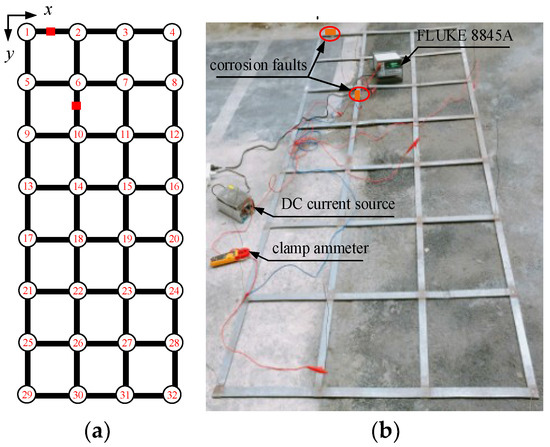
Figure 11.
The experimental picture. (a) The simulated grounding grid model; (b) The experiment picture.
In the experiment, the cycle measurement method introduced in Section 3.1 is used to acquire potential data, the dataset contains 1141 measurements. The measurement data in one time are shown in the Table 2, where the current inflow node is 30, the outflow node is 19 and the potential reference node is 29, in order to reduce the error in the data, the potentials of the current inflow point and the outflow point are removed.
Table 2.
A part of the measurements.
There are two artificial corrosion faults set in the grounding grid, the resistivity contrast measured is 8:1, the imaging result obtained in Figure 12. Due to the noise of the measurements, the resolution of the grounding grid gets a little poor but it can still locate corrosion faults correctly.
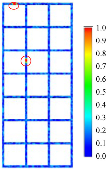
Figure 12.
The result of corrosion diagnosis on the simulated grounding grid.
5.2. Field Experiment
A 220 kV substation in the southeast China was selected to do the corrosion diagnosis experiment with EIT. The structure of this substation is shown in Figure 13.
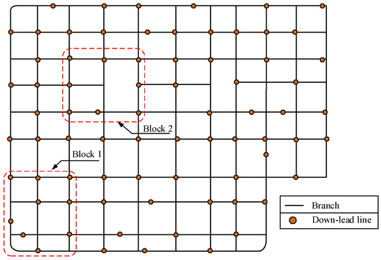
Figure 13.
The structure of a 220 kV grounding grid.
In the field experiment, the 16-channel potential acquisition instrument is used to measure the potentials. We focus on two blocks (shown in Figure 13) in the ground grid and use EIT to reconstruct the resistivity distribution. The experimental picture and imaging results are shown in Figure 14. In the imaging results about the resistivity distribution, a few parts of the branches have been corroded. The corrosion in the block 2 is more serious and the intersection point of the branch is more prone to corrosion in both two blocks. The reason maybe that there is a greater leakage current from the equipment in the center of the grounding grid and cause more serious electrochemical corrosion. We dug half of the right branch of the block 2 and found one corrosion in the branch, which reaches a good agreement with the imaging result.

Figure 14.
The experiment picture and imaging results on the field experiment, (a) the experimental setup; (b) the imaging results of block 1 and block 2; (c) one eroded branch dug from the block 2.
Therefore, form the experiments above, the correctness and feasibility of grounding grid EIT are verified, it can be used to do the corrosion detection in the substation.
6. Conclusions
In this paper, a method of grounding grid corrosion diagnosis is put forward based on the electrical impedance tomography technique, which focus on the distribution parameter, resistivity of grounding grid branch but not the resistor value of the branch, so it can locate the accurate corrosion point in the branch. The theoretical analysis and experiments verified that the method can locate the corrosion faults of the grounding grid clearly and accurately. Through the resistivity distribution imaging, the location and the corrosion degree can be judged clearly. The soil-separation and block-diagnosis methods can improve the resolution and imaging efficiency. In the present work, the sufficient measurements and the construction structure are the important factors affecting the imaging resolution, so in our further work, we will mainly focus on the data interpolation method and image processing method to improve the imaging resolution.
Author Contributions
Conceptualization, X.L. and F.Y.; Data curation, S.H.; Funding acquisition, F.Y. and J.M.; Investigation, X.L.; Methodology, X.L.; Software, S.H.; Validation, J.M.; Writing—original draft, X.L.; Writing—review & editing, A.J.
Funding
This work was founded by the National Natural Science Foundation of China (No. 51477013) and Chongqing University Postgraduates’ Innovation Project (No. CYS15011).
Acknowledgments
This work was supported by the National Natural Science Foundation of China (No. 51477013) and the technology project of Hangzhou Yineng Electric Technology Co., Ltd. (EPRD2017-07).
Conflicts of Interest
The authors declare no conflict of interest.
References
- Yu, C.G.; Fu, Z.H.; Wu, G.L.; Zhou, L.Y.; Zhu, X.G.; Bao, M.H. Configuration detection of substation grounding grid using transient electromagnetic method. IEEE Trans. Ind. Electron. 2017, 64, 6745–6783. [Google Scholar] [CrossRef]
- Ackerman, A.; Sen, P.K.; Oertli, C. Designing safe and reliable grounding in AC substations with poor soil resistivity: An interpretation of IEEE Std. 80. IEEE Trans. Ind. Appl. 2013, 49, 1883–1889. [Google Scholar] [CrossRef]
- Ko, J.W.; Cha, H.L.; Kim, D.K.-S.; Lim, J.R.; Kim, G.G.; Bhang, B.G.; Won, C.S.; Jung, H.S.; Kang, D.H.; Ahn, H.K. Safety analysis of grounding resistance with depth of water for floating PVs. Energies 2017, 10, 1304. [Google Scholar] [CrossRef]
- Zhang, B.; Jiang, Y.K.; Wu, J.P.; He, J.L. Influence of potential difference within large grounding grid on fault current division factor. IEEE Trans. Power Deliv. 2014, 29, 1752–1759. [Google Scholar] [CrossRef]
- Harid, N.; Griffiths, H.; Mousa, S.; Clark, D.; Robson, S.; Haddad, A. On the analysis of impulse test results on grounding systems. IEEE Trans. Ind. Appl. 2015, 51, 5324–5334. [Google Scholar] [CrossRef]
- Zhu, Y.; Li, Y.P.; Sang, J.B.; Bao, M.L.; Zang, H.X. Analysis and improvement of adaptive coefficient third harmonic voltage differential stator grounding protection. Energies 2018, 11, 1430. [Google Scholar] [CrossRef]
- Zhu, X.S.; Cao, L.L.; Yao, J.F.; Yang, L.; Zhao, D. Research on ground grid diagnosis with topological decomposition and node voltage method. In Proceedings of the 2012 Spring Congress on Engineering and Technology, Xian, China, 27–30 May 2012; pp. 1–4. [Google Scholar]
- Xu, L.; Li, L. Fault diagnosis for grounding grids based on electric network theory. Trans. China Electrotech. Soc. 2012, 27, 270–276. [Google Scholar]
- Hu, J.Y.; Hu, J.G.; Lan, D.L.; Ming, J.L.; Zhou, Y.T.; Li, Y.W. Corrosion evaluation of the grounding grid in transformer substation using electrical impedance tomography technology. In Proceedings of the IEEE Industrial Electronics Society, Beijing, China, 18 November 2017; pp. 5033–5038. [Google Scholar]
- Zhang, B.; Zhao, Z.B.; Cui, X.; Li, L. Diagnosis of breaks in substation's grounding grid by using the electromagnetic method. IEEE Trans. Magn. 2002, 38, 473–476. [Google Scholar] [CrossRef]
- Yu, C.G.; Fu, Z.H.; Wang, Q.; Tai, H.M.; Qin, S.Q. A novel method for fault diagnosis of grounding grids. IEEE Trans. Ind. Appl. 2015, 51, 5182–5188. [Google Scholar] [CrossRef]
- Yu, C.G.; Fu, Z.H.; Hou, X.Z.; Tai, H.M.; Su, X.F. Break-point diagnosis of grounding grids using transient electromagnetic apparent resistivity imaging. IEEE Trans. Power Deliv. 2015, 30, 2485–2491. [Google Scholar] [CrossRef]
- Liu, K.; Yang, F.; Zhang, S.Y.; Zhu, L.W.; Hu, J.Y.; Wang, X.Y.; Irfan, U. Research on grounding grids imaging reconstruction based on magnetic detection electrical impedance tomography. IEEE Trans. Magn. 2018, 54, 1–4. [Google Scholar] [CrossRef]
- Braun, F.; Proenca, M.; Sola, J.; Thiran, J.; Adler, A.A. Versatile noise performance metric for electrical impedance tomography algorithms. IEEE Trans. Biomed. Eng. 2017, 64, 2321–2330. [Google Scholar] [CrossRef] [PubMed]
- Murphy, E.; Mahara, A.; Halter, R. Absolute reconstructions using rotational electrical impedance tomography for breast cancer imaging. IEEE Trans. Med. Imag. 2016. 36, 892–903. [CrossRef]
- Yang, Y.J.; Jia, J.B.; Smith, S.; Jamil, N.; Gamal, W.; Bagnaninchi, P. A miniature electrical impedance tomography sensor and 3D image reconstruction for cell imaging. IEEE Sens. J. 2017, 17, 514–523. [Google Scholar] [CrossRef]
- Li, C.L.; He, W.; Yao, D.G.; Yang, F.; Kou, X.K.; Wang, X.Y. Topological measurement and characterization of substation grounding grids based on derivative method. Int. J. Eelectron. Power 2014, 63, 158–164. [Google Scholar]
- Fu, Z.H.; Song, S.Y.; Wang, X.J.; Li, J.Q.; Tai, H.M. Imaging the topology of grounding grids based on wavelet edge detection. IEEE Trans. Magn. 2018, 54, 1–8. [Google Scholar] [CrossRef]
- Susanne, B.; Ridgway, S. The Mathematical Theory of Finite Element Method, 3rd ed.; Texts in Applied Mathematics: California, CA, USA, 2008; pp. 155–172. [Google Scholar]
- Hofmann, B. Penalty methods for the inverse problem in EIT. Physiol. Meas. 1996, 17, A73. [Google Scholar] [CrossRef] [PubMed]
- Johnston, R.; Gulrajani, M. Selecting the corner in the L-curve approach to Tikhonov regularization. IEEE Trans. Biomed. Eng. 2000, 47, 1293–1396. [Google Scholar] [CrossRef] [PubMed]
- Yang, F.; Wang, Y.A.; Dong, M.L.; Kou, X.K.; Yao, D.G.; Li, X.; Gao, B.; Irfan, U. A cycle voltage measurement method and application in grounding grids fault location. Energies 2017, 10, 1929. [Google Scholar] [CrossRef]


© 2018 by the authors. Licensee MDPI, Basel, Switzerland. This article is an open access article distributed under the terms and conditions of the Creative Commons Attribution (CC BY) license (http://creativecommons.org/licenses/by/4.0/).