Traveling Wave Fault Location Using Layer Peeling

Abstract

Many fault-location algorithms rely on a simulation model incorporating network parameters which closely represent the real network. Estimations of the line parameters are usually based on limited geometrical information which do not reflect the complexity of a real network. In practice, obtaining an accurate model of the network is difficult without comprehensive field measurements of each constituent part of the network in question. Layer-peeling algorithms offer a solution to this problem by providing a fast “mapping” of the network based only on the response of a probing impulse. Starting with the classical “Schur” layer-peeling algorithm, this paper develops a new approach to map the reflection coefficients of an electrical network, then use this information post-fault to determine accurately and robustly the location of either permanent or incipient faults on overhead networks. The robustness of the method is derived from the similarity between the post-fault energy reaching the observation point and the predicted energy, which is based on real network observations rather than a simulation model. The method is shown to perform well for different noise levels and fault inception angles on the IEEE 13-bus network, indicating that the method is well suited to radial distribution networks.

1. Introduction

1.1. Motivation

Most customer interruptions originate on the Medium Voltage (MV) network [1]. In terms of fault location, such networks can have several challenging characteristics, including tapped loads, radial topologies, and mixed overhead/cable lines. Moreover, in rural and semi-urban networks, the relativity low concentration of customers means that any new investment in fault-location improvement usually needs to be low cost to be economically justifiable. This work proposes a new traveling wave fault-location method which requires only a single observation point yet can locate faults on highly branched networks with tapped transformer loads at arbitrary positions.

1.2. Literature Review

In this section, a brief review of the state-of-the-art in fault location is presented. Fault location algorithms broadly fall into two main categories; impedance-based methods and traveling wave methods. Impedance-based methods attempt to calculate the distance to the fault based on measurements of impedance. Single-ended methods require observations from only one end of the line. The simplest type of single-ended method is known as the reactance method. It attempts to estimate the distance to fault based on the assumption that the farther away the fault point, the greater the overall post-fault impedance, and vice-versa. The fault impedance, i.e., the portion of the impedance made up of the fault itself, is considered to be purely resistive. The simple reactance method encounters problems when the fault current is not in phase with the observed current at the relay, a mismatch attributed to the effect of the load [2]. Takagi’s method, which represented a significant improvement, attempted to eliminate this mismatch using pre-fault [3], or zero-sequence current as measured by the relay [4]. Eriksson’s approach uses network impedance data to more accurately account for remote source infeed [5]. Double-ended (and multi-end) impedance-based methods operate on a similar principle to single-ended methods, though instead use observations from relays on both ends of the line [4,6]. Synchronized double-ended methods require that both ends of the line have access to a synchronized time reference, e.g., GPS or GLONASS. Where access to a time reference is not available, double-ended methods can still be used [7]. Recent efforts have been made to extend the applicability of impedance-based methods, which are normally valid only on single circuit transmission and point to point distribution lines. In [8], a new method is presented which explicitly handles double-circuit lines. In [9,10], new methods are proposed to overcome the multiple-estimation problem and extend the use of impedance-based methods to radial distribution systems. A priority in the field is the development of methods which are robust in the presence of distributed generation. A promising development in this area is the emergence of synchrophasor-based methods with real-time estimation [11,12].

Traveling wave methods rely on the fact that when a fault occurs in an electrical network, it initiates a high-frequency disturbance which propagates in both directions away from the fault point. A fault recorder placed within the network will record the convolution of the signal at the fault point and the impulse response separating its location and the fault point. Many fault-location algorithms restrict themselves to the early part of this convolution, using the relative timestamps of the first few impulses arriving at the fault recorder, and an assumption about the speed of the signals, to arrive at an estimate of the fault-location [13]. In [14], a comparison between the measured differences in arrival times and a set of network derived differences is used. The equivalency between the differences in post-fault arrival times and the expected arrival times based on network data allows a metric to be formed which minimizes at the faulted point. However, for full coverage of a network, time-synchronized fault recorders are required in both directions from any theoretical fault position; a condition which is expensive to satisfy on highly branched networks, especially those in rural areas. Other methods, for example the recently proposed time-reversal method [15], back-inject the reversed fault recorder signal into a simulation model of the network with the understanding that the energy will maximize at the origin of the fault. This represents, in effect, a convolution of the observed signal with the full impulse responses separating the position of the fault recorder and all possible locations in the network. In theory, a fault can be identified from a single observation point. Crucial to this method is an accurate representation of the network in the simulation environment, yet the complexity of a typical electrical network makes the modelling problem extremely difficult. Another general problem with traveling wave methods is the difficulty in detecting, and time-stamping, the fault-induced transients. In the last few decades, the use of the wavelet transform has emerged to improve detection of high-frequency traveling waves [16,17,18]. Previous works have identified the Daubechies 4 (db4) mother wavelet as appropriate for the detection of high-frequency traveling waves in electrical networks [19,20]. A comprehensive review of feature extraction methods in high voltage fault-location applications is given by [21].

Recently, new fault-location methods which do not fit nicely into either of the previously discussed classifications have emerged. In [22], voltage sag information from dispersed smart meters is used to calculate the faulted bus. The trend of using emerging monitoring infrastructure is further demonstrated by [23], which uses Phasor Measurement Units (PMUs) on transmission networks, and [24], which proposes a method based on $\mu$PMU measurements on distribution networks. Another notable emerging trend is the use of syntactic pattern recognition to detect faults [25].

1.3. New Approach

One of the main problems associated with models-based traveling wave methods is the mismatch between the real network and the simulation model. One possible way to resolve this is to measure directly the impulse responses separating each part of the network and the fault recorder. In theory, this could be done by injecting an impulse at the position of the fault recorder and measuring the response at discrete intervals in the network. If this operation is carried out correctly, the time-reversal method could be executed using actual network data rather than a model. However, such a procedure is too time consuming and onerous to be practical.

A more practical approach is to attempt to “map out” the network using Time Domain Reflectometry (TDR). In simple terms, this involves injecting an impulse into a line and recording the reflections at the same point. The trail of reflected pulses can be analyzed to reveal the reflection coefficients, their electrical distance down the line and the characteristic impedance of each section. A similar approach is used extensively in seismology to map out the characteristics of the layered earth [26,27]. In fact, such an approach can be used to solve the inverse problem in any kind of problem characterized by the propagation of a signal through inhomogeneous media. The algorithms have grown more sophisticated over time, though most relate closely to the classical Schur Algorithm [28] and involve “layer peeling” to recursively determine the reflection coefficient of each layer, starting with the nearest to the probing impulse. In this work, a practical implementation of the pulse injection is proposed based on the use of the capacitive divider built into the Voltage Detection Systems (VDS), which must be installed in all MV switchboards according to IEC 61243-5. The concept was recently introduced for applications in Power Line Communication (PLC) coupling [29].

This work adapts the layer-peeling method and demonstrates its use on overhead networks modelled on 11 kV wood pole lines. Tapped transformers, which behave as reflectors, are placed at intervals along the line/network and identified using the layer-peeling algorithm. The mapped reflection coefficients are then used as the basis for a practical and robust fault-location algorithm.

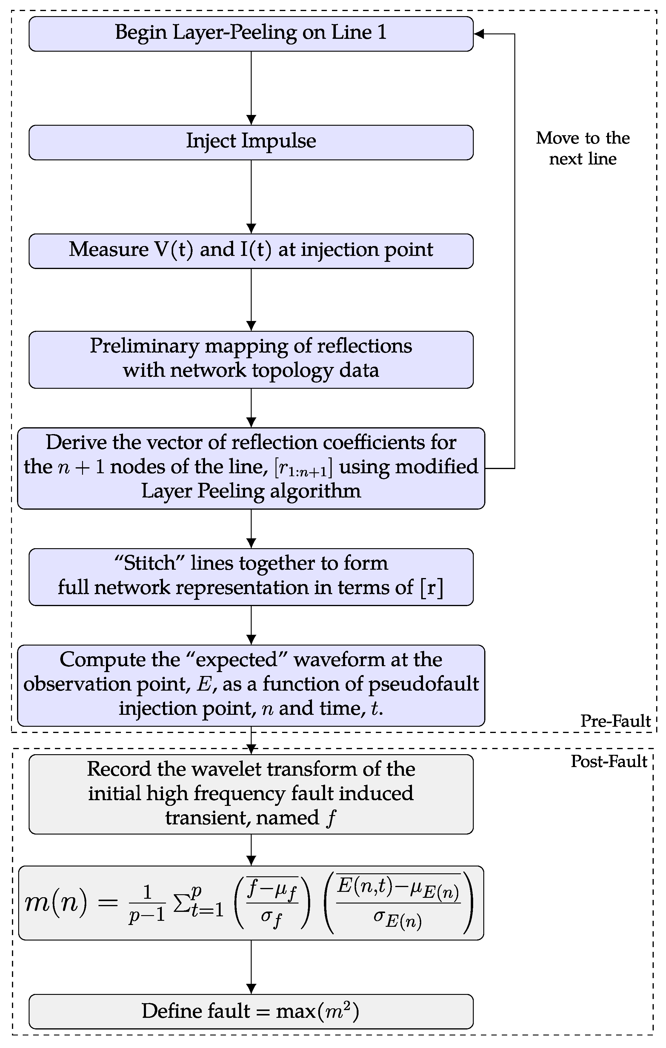
2. Overview of the Proposed Method

In theory, a fault can be located based on the arrival time(s) of the initial, induced traveling wave at one, or several observation points [14,30,31]. However, the procedure is complicated by the presence of internal reflection points which are sometimes not accounted for in traditional traveling wave algorithms, or impossible to predict in models-based approaches. There are notable examples of field-based studies which have attempted to resolve this problem [32,33]. An example of a reflector whose precise location is difficult to know with accuracy a tapped transformer, many of which are likely to be present on a typical distribution feeder. If it is known a priori where these reflectors are, the network can be mapped such that the “expected” sequence of arriving traveling waves for a fault at any location on the network may also be known to a high degree of accuracy.

To further explain the method, consider the transmission line of Figure 1. It has an “internal” reflector in the form of a tapped transformer, plus a terminating transformer at the far end of the line. Assume that the distance of the mid-line transformer from the source is known to be, say, 57 m, and the total length of the line is 100 m. With this knowledge, it is possible to sketch out the expected arrival times of the first several fault-induced traveling waves as a function of fault position, with or without the fault impedance. A convenient way to show the range of expected arrival sequences is to plot the received energy as a function of both injected network position (i.e., the node at which the theoretical impulse is injected) and time. In this case, a binary decision is made on whether a pulse has arrived using a simple comparison with a predesignated threshold value, set as a percentage of the magnitude of the first arriving pulse (a value of around 20% was used in this work). Drawing a vertical cursor at a node injection point shows the expected arrival time of pulses for a fault at that location. The expected sequence, using the first arrived pulse as a reference line, can be compared with the observed, fault-induced energy arriving at the observation point, with the most similar sequence chosen as the location of the fault. Previous work has shown the utility in using the Wavelet Transform for isolating high-frequency disturbances from the immediate post-fault waveform, thus revealing a sequence of pulses matching what would be the impulse response from the fault point to the observation point [16,19,20,34]. In this work, the received fault signal, after wavelet transformation, is represented by the function $f\left(t\right)$. Let the “expected” signal be a function of node injection point, n and time: $E(n,t)$, where E is a matrix of n columns, each representing the sequence of arrived pulses for a theoretical fault at node n. Please note that the reference line has a negative slope. Therefore, to compare the similarity of f and the n rows of E, the matrix form of E is rotated counter-clockwise until the reference line is horizontal (Figure 1b is converted to Figure 1c). Inspection of each column of E shows the time intervals within which energy from the fault-induced transient is expected to arrive at the observation point. This can be exploited by forming a metric, $m\left(n\right)$, shown in Equation (1), which correlates f with each column of E. A strong correlation is expected in the particular column of E which matches f.

$$m\left(n\right)=\frac{1}{p-1}\sum _{t=1}^p\left(\frac{\overline{f-{\mu }_f}}{{\sigma }_f}\right)\left(\frac{\overline{E(n,t)-{\mu }_{E\left(n\right)}}}{{\sigma }_{E\left(n\right)}}\right)$$

(1)

where p = $t_{max}$, ${\mu }_f$ and ${\mu }_{E\left(n\right)}$ are the mean and ${\sigma }_f$ and ${\sigma }_{E\left(n\right)}$ are the standard deviations of the fault and nth column of the expected matrix, E, respectively. The correlation can be made stronger by exploiting knowledge of the polarity of the reflection coefficients within the network without necessarily knowing the precise magnitude.

The proposed method depends on there being n unique sequences at a chosen $t_{max}$ to avoid the possibility of conflicts in the fault estimation. This can be tested by finding the correlation coefficient matrix describing the relationship between each mutual pair of columns in E. It is shown later that except in cases of extreme symmetry, which is highly unlikely on a real distribution network, the condition of n unique sequences is indeed satisfied and later proven for the example networks.

This paper begins by showing how the precise location (and possibly the magnitude) of the reflection coefficients along a line can be calculated. Once these are known for each line, it is shown how they can be “stitched” together to form a complete representation of the network. To facilitate the method, a novel, simplified line model is developed to help use the network mapped reflection coefficients to calculate the vectors of expected impulse responses at each node in the network (a prerequisite for the similarity check and fault-location estimation). The line model can “broaden” the impulse as it travels through the network, replicating the spreading out of energy. Finally, the method is tested using single line and teed examples.

3. Layer Peeling for Lossy Electrical Networks

The aim of layer peeling is to calculate recursively the reflection coefficients of a multilayered media [35]. The usual starting point is to probe the media with an impulse-like signal then record the sequence of reflected pulses. This section will provide a brief overview of the generic layer-peeling algorithm and propose modifications to improve its suitability for measuring the reflectivity vector for a distribution or transmission line.

The transmission line shown in Figure 1 is split evenly into $n+1$ nodes. $r_1$ to $r_{n-1}$ denote the reflection coefficient at each of the non-terminating nodes. If a transmission line is split up into reasonably small discrete intervals, for example 3 m, most reflection coefficients will be zero, meaning all the signal passes through with no reflection. However, due to the presence of tapped transformers, characteristic impedance transitions (i.e., cable to OHL) and any other discontinuities, some nodes will exhibit a non-zero reflection coefficient. This reflection coefficient, $\mathsf{\Gamma }$, can be found in terms of the change in characteristic impedance between the portion of line to the left and right of the discontinuity at position $r_k$:

$$\mathsf{\Gamma }=\frac{Z_k-Z_{k-1}}{Z_k+Z_{k-1}}$$

(2)

where k represents an arbitrary position along the line. For a discontinuity appearing as a load in parallel with the line, or to ground, where the characteristic impedance remains unchanged either side, $\mathsf{\Gamma }$ takes a different form:

$$\mathsf{\Gamma }=\frac{-Z_k}{Z_k+2Z_L}$$

(3)

where $Z_L$ is the impedance presented at the discontinuity. The distinction between Equations (2) and (3) shows that the layer-peeling algorithm must have knowledge of whether the reflection at a given node is due to an impedance mismatch or a parallel impedance to properly calculate $\mathsf{\Gamma }$. This can be estimated to a good degree of accuracy by consulting network topology data, with the assumption that any reflection that is not sufficiently nearby a cable/OHL transition is caused by a parallel impedance such as a tapped transformer. Please note that the prior analysis assumes a frequency-independent characteristic impedance. In this work, this assumption is put forward since it has been shown that $Z_k$ is indeed frequency-independent in the high-frequency region [36].

An alternative method to define $\mathsf{\Gamma }$ is in terms of a left and right propagating wave:

$$\mathsf{\Gamma }=\frac{w_L(k,t)}{w_R(k,t)}$$

(4)

where $w_L$ and $w_R$ are the left and right propagating waves, respectively. Please note that the directional waves are functions of position on the line, k and time, t. The conversion of voltage and current to $w_L$ and $w_R$ is a change of variables that was first introduced by Snelson [37].

$$w_R(n,t)=\frac{V(n,t)+Z_{k}I(n,t)}{2}$$

(5)

$$w_L(n,t)=\frac{V(n,t)-Z_{k}I(n,t)}{2}$$

(6)

The use of left and right propagating wave variables (as opposed to voltage current directly) holds the advantage of providing a more intuitive analysis of the layer-peeling algorithm, and, as will be explained later, is advantageous in the development of a frequency-dependent line modelling solution.

The layer-peeling algorithm, assuming for now that the line is lossless, commences as follows:

• An impulse is injected into the line from position $r_o$.
• The voltage and current at the point of impulse injection is recorded.
• Calculate $w_L(0,t)$ and $w_R(0,t)$ from Equations (5) and (6), that is, the reflected impulse response at the point of injection.
• Calculate the reflection coefficient of the first reflector, ${\mathsf{\Gamma }}_{rf1}$ using

  $${\mathsf{\Gamma }}_{rf1}=\frac{w_L(0,t+\alpha )}{w_R(0,t)}$$

  where $\alpha$ is the time delay between the injected impulse and the first returning pulse.
• Infer $w_R(1,t)$ by “propagating” $w_R(0,t)$ through ${\mathsf{\Gamma }}_{rf1}$. Infer $w_L(1,t)$ by “reverse propagating” $w_L(0,t)$ through ${\mathsf{\Gamma }}_{rf1}$.
• Calculate the reflection coefficient of the second reflector, ${\mathsf{\Gamma }}_{rf2}$ using

  $${\mathsf{\Gamma }}_{rf2}=\frac{w_L(1,t+\beta )}{w_R(1,t)}$$

  where $\beta$ is the time delay between the second returning pulse and the third returning pulse.
• Continue the process until a sufficient depth into the line has been reached.

The meaning of “propagate” and “reverse propagate” in item 5 of the procedure above is fundamental to the way in which the layer-peeling algorithm works. Given that the previous layer’s left and right propagating waves, and the reflection coefficient to the next layer, are known, the algorithm can estimate the subsequent layer’s wave variables at the next reflector, and so the process continues. The right propagating wave is “propagated” through the most recently calculated reflection coefficient in the same manner as the real-life equivalent propagates through. However, the calculation of the next layer’s left propagating variable must reverse the effect of all of the transmission coefficients which separate the point of the reflection with the relevant observed pulse at the source. In other words, the algorithm works out the right propagating variable by performing a recursive forward simulation and the left propagating variable by performing a backward (reversed-time) simulation.

3.1. Correcting for Lossy Lines

The description above is valid for lossless transmission lines. In a lossy line, the situation is complicated because one can no longer assume that the ratios of pulses observed at the source are only due to the various reflection coefficients along the line. Instead, the ratios will also be affected by attenuation and dispersion. The longer the line, the greater the scope for deviation between the recorded and actual reflection coefficients.

To account for attenuation, a correction factor is proposed. This is designed to artificially increase and decrease the amplitude of the left and right propagating variables, respectively. For the first section of the hypothetical example described earlier, $\mathsf{\Gamma }$ becomes:

$$\mathsf{\Gamma }=\frac{w_L(0,t)\left({\zeta }^{\alpha /2}\right)}{w_R(0,t)\left({\left(\frac{1}{\zeta }\right)}^{\alpha /2}\right)}$$

(7)

where $\zeta$ is the attenuation per meter. The same correction factor is applied to subsequent calculations of $\mathsf{\Gamma }$, except with the time delay variable (in this case $\alpha$, which represents the distance between the reflectors, replaced by the appropriate value. The value of $\zeta$ will also vary depending on the nature of the transmission line, though it will be shown later that only a rough estimation is required for the proposed algorithm to work accurately.

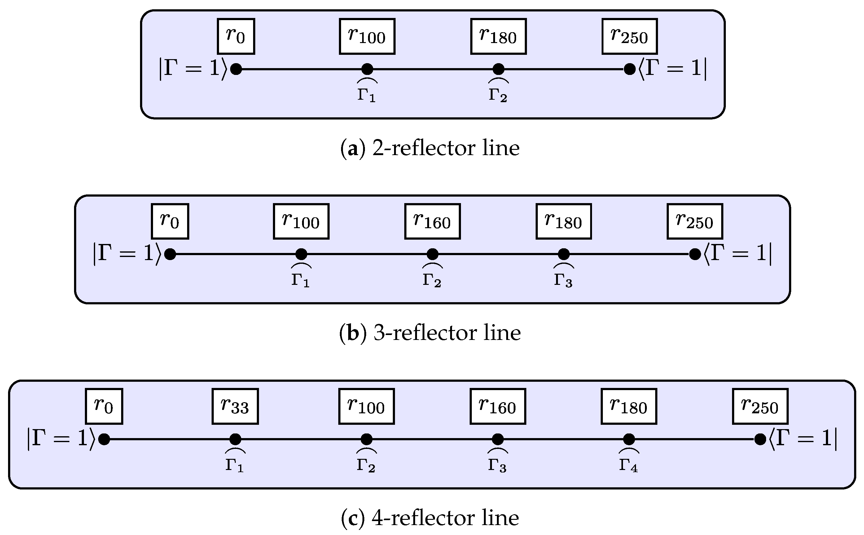
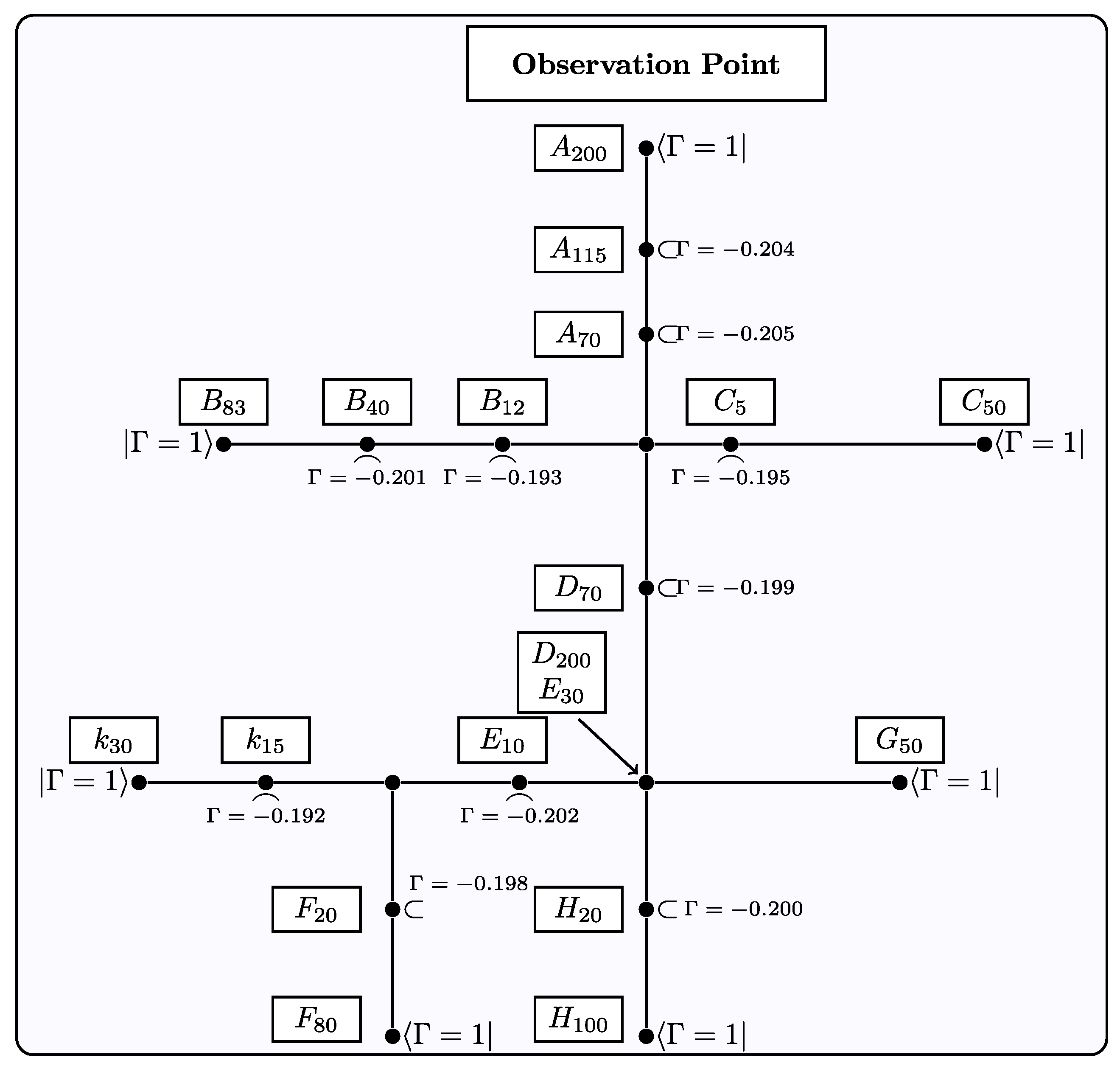
3.2. Accounting for Internal Reflections

Another potential problem with the classical layer-peeling algorithm is its inability to distinguish between genuine returning pulses (i.e., those which result from a direct and initial trip between the source, the reflector and back again) and those which internally change direction more than once before returning to the injection point. The algorithm may therefore mistake a returning pulse as a genuine reflection from some depth into the line when in fact it is the result of an internal pattern of reflections closer to the source. One possibility to resolve this problem is to prevent the algorithm from looking for reflectors at time intervals when returning pulses from internal reflections are expected to arrive back at the injection point. For example, if the first returning pulse arrives $t_1$ seconds after the original impulse is injected, it is expected that subsequent pulses will arrive at $2t_1$, $4t_1$, $6t_1$ and so on. The algorithm can automatically exclude these pulses from the calculations. Of course, as the reflection coefficients of the line are recursively revealed, the regions of time excluded will grow rapidly due both to dispersion of the pulse and a growing number of possible paths for the signal to take. There is also a possibility that a genuine reflection will fall within an exclusion period. The likelihood of this depends on the distance between the reflectors, the dispersion of the line and the width of the pulse.

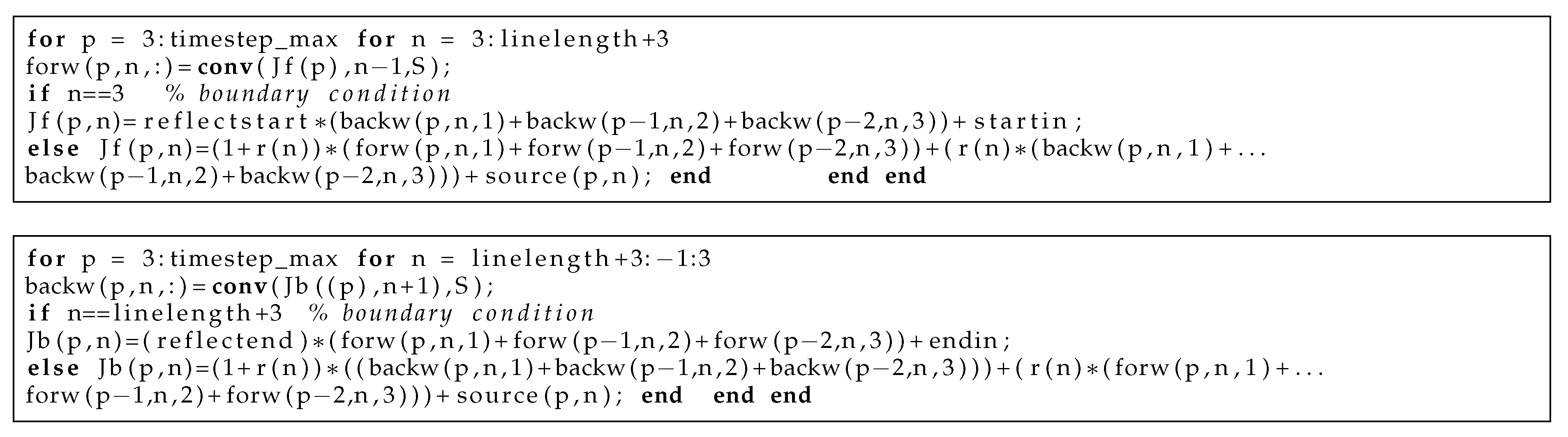
4. Calculating Impulse Responses Based on the Derived Reflection Coefficients

The next phase of the algorithm requires that the impulse responses from all nodes within the line (or network), to the injection/observation point, are constructed based on the previously calculated reflection coefficients. To do this, the concept of the left and right propagating variables, as described in Section 3 is retained, but here it will be used to derive a simplified line model. This line model will provide the basis of the impulse response estimation.

The fault-location algorithm depends on the time at which the energy of the impulse response derived from the fault arrives at the observation point. For this reason, it is important to model the way in which the impulse disperses as it propagates. This is usually accomplished through the use of “weighting functions”, which are convolved with the directional wave variables to model the frequency-dependent propagation from the start to the end point of a line, a method proposed by Snelson [37] and later incorporated into the popular frequency-dependent line model by J. Marti [36]. The “fatter” the weighting function, the greater the dispersion will be. The convolution integral is bounded at its lower limit by the time delay of the fastest frequency component and at its upper limit by the slowest.

To facilitate the proposed method, the impulse response separating each node and the observation point must be calculated. This is most conveniently achieved in a computational loop, with a pulse injected at a slightly different position at each iteration. This means that each iteration would also need to invoke a line model with slightly different weighting functions due to the lengths of line sections growing slightly shorter and longer either side of the injection point. Instead, this work proposes a miniaturization of the line model to the smallest possible length i.e., the distance between nodes. Now, the length of the convolution integral is reduced to just 3 samples. The first sample is zero (representing a delay by one timestep). The second and third samples of the weighting function are non-zero, with the second significantly larger than the third. Figure 2 shows MATLAB code for the implementation of the line model which calculates the forward and backward waves, respectively. The convenience of such a representation is derived from the ability to model the propagation of an impulse on a node by node, timestep by timestep basis. An overview of the proposed algorithm in its entirety is shown in Figure 3.

5. Case Studies

5.1. Single Line

Figure 4a–c shows single lines with 2, 3 and 4 internal reflectors, respectively. The reflectors are positioned at arbitrary positions along the line and are considered tapped discontinuities, matching the effect of a tapped transformer. In these cases, each node represents 3 m, so each line is 750 m long. Each line is modelled in the EMTP-ATP as a three-phase 11 kV distribution line using frequency-dependent (JMarti) line models. The geometry and resistivity of the line and the chosen earth resistivity are shown in

Table 1. Characteristics of the OHTL and Simulation Parameters.

11 kV Wood Pole Overhead Line
Height, h	9 m
Height at mid-span, $h_{mid}$	7.5 m
Conductor separation, d	1.5 m
Conductor name	Dingo
Conductor core area	158.7 mm2
Conductor resistivity	0.1814 $\mathsf{\Omega }$/km DC
Earth resistivity	100 $\mathsf{\Omega }$·m
EMTP Simulation Parameters
Sampling Frequency	100 MHz
Pulse Width for TDR	$5\times {10}^{-8}$ s

.

Throughout this work, aerial mode 2 (the natural mode of propagation involving the two-outer conductors) is used. This is extracted from the simulation environment during runtime using a Fortran model which performs the phase to mode conversion based on the transformation matrix calculated in the Line and Cables Constants (LCC) routine of the EMTP. For the pre-fault portion of the algorithm (i.e., layer peeling and derivation of E), the mode 2 quantity at the point(s) of injection are first exported from the EMTP-ATP to MATLAB. Similarly, the post-fault mode 2 quantity from a single observation point is exported to MATLAB and prepared for the next stage: the layer-peeling routine.

5.1.1. Step 1: Layer Peeling

The procedure outlined in Section 3 is carried out on each of the single line networks. In these cases, a correction factor, $\zeta$, of 0.999 is used. This is derived as an approximation based on the attenuation reported by the LCC routine.

Table 2. Actual versus Calculated (using Layer-Peeling) Reflection Coefficients ($Z_c$ = 292 $\mathsf{\Omega }$).

Line		${\mathsf{\Gamma }}_{\mathbf{1}}$			${\mathsf{\Gamma }}_{\mathbf{2}}$			${\mathsf{\Gamma }}_{\mathbf{3}}$			${\mathsf{\Gamma }}_{\mathbf{4}}$
		Actual	Calculated	$\mathsf{\Delta }$ (%)	Actual	Calculated	$\mathsf{\Delta }$ (%)	Actual	Calculated	$\mathsf{\Delta }$ (%)	Actual	Calculated	$\mathsf{\Delta }$ (%)
1.1	$\mathsf{\Gamma }$	−0.1721	−0.1719	−0.12	−0.1721	−0.1650	−4.3
	$\mathsf{\Omega }$	700 $\mathsf{\Omega }$	699.2 $\mathsf{\Omega }$		700 $\mathsf{\Omega }$	671.1 $\mathsf{\Omega }$
1.2	$\mathsf{\Gamma }$	−0.2260	−0.2241	−0.58	−0.1274	−0.1347	+5.7
	$\mathsf{\Omega }$	500 $\mathsf{\Omega }$	495.8 $\mathsf{\Omega }$		1000 $\mathsf{\Omega }$	1057.3 $\mathsf{\Omega }$
2.1	$\mathsf{\Gamma }$	−0.1721	−0.1719	−0.12	−0.1721	−0.1650	−4.3	−0.1721	−0.1627	−5.8
	$\mathsf{\Omega }$	700 $\mathsf{\Omega }$	699.2 $\mathsf{\Omega }$		700 $\mathsf{\Omega }$	671.1 $\mathsf{\Omega }$		700 $\mathsf{\Omega }$	661.8 $\mathsf{\Omega }$
2.2	$\mathsf{\Gamma }$	−0.2674	−0.2664	−0.38	−0.1172	−0.1119	−4.74	−0.2260	−0.2095	−7.9
	$\mathsf{\Omega }$	400 $\mathsf{\Omega }$	398.5 $\mathsf{\Omega }$		1100 $\mathsf{\Omega }$	1050.3 $\mathsf{\Omega }$		500 $\mathsf{\Omega }$	463.5 $\mathsf{\Omega }$
3.1	$\mathsf{\Gamma }$	−0.1721	−0.1719	−0.12	−0.1721	−0.1650	−4.3	−0.1721	−0.1627	−5.8	−0.1721	−0.1695	−1.51
	$\mathsf{\Omega }$	700 $\mathsf{\Omega }$	699.2 $\mathsf{\Omega }$		700 $\mathsf{\Omega }$	671.1 $\mathsf{\Omega }$		700 $\mathsf{\Omega }$	661.8 $\mathsf{\Omega }$		700 $\mathsf{\Omega }$	693.5 $\mathsf{\Omega }$
3.2	$\mathsf{\Gamma }$	−0.1543	−0.1537	−0.39	−0.2260	−0.2161	−4.6	−0.3274	−0.3055	−7.2	−0.1172	−0.1099	−6.64
	$\mathsf{\Omega }$	800 $\mathsf{\Omega }$	796.9 $\mathsf{\Omega }$		500 $\mathsf{\Omega }$	478.1 $\mathsf{\Omega }$		300 $\mathsf{\Omega }$	279.9 $\mathsf{\Omega }$		1100 $\mathsf{\Omega }$	1031.5 $\mathsf{\Omega }$

. The values of actual $\gamma$, and the estimates derived from the layer-peeling process, are shown for the 6 single line types are shown in Table 2.

5.1.2. Step 2: Derivation of E

The newly acquired vector of reflectors, r, can now be incorporated into the simulation outlined in Section 4 to derive the expected waveform at the observation point at the start of the line ($r_0$). This is done by injecting a pseudofault (an impulse) into the network at each node and recording the arrived pulses at the observation point. For the single line networks considered here, 250 separate simulations are performed to derive the 250 column vectors making up E. The matrix E is subsequently rotated counter-clockwise such that the reference line (i.e., the line representing the first arrived pulse at the observation point) is horizontal.

At this stage, E has elements with numerical entries representing the polarity and magnitude of the observed waveform due to the pseudofault impulse. It has been found useful to discretize the entries of E into three possible values: 1, −1 and 0. This is achieved using a comparison with a threshold value, $E_{threshold}$, according to the following equation:

$$E_b(n,p)=\left\{\begin{array}{cc}1,\hfill & \mathrm{if}E(n,p)\ge E_{threshold}\hfill \\ -1,\hfill & \mathrm{if}E(n,p)\le -E_{threshold}\hfill \\ 0,\hfill & \mathrm{otherwise}\hfill \end{array}\right.$$

(8)

The same discretization is performed on f post-fault. This has been found to strengthen the correlation at the correct fault point and weaken the correlation elsewhere. Figure 5a shows a plot of $E_b$ corresponding to the 2-reflector line, with a fault impedance of 10 $\mathsf{\Omega }$. Note how the lines become thicker towards the bottom-right, representing the greater dispersion of the pulse with distance traveled. Figure 5b shows the coefficient correlation matrix for the 2-reflector line i.e., the correlation between each mutual pair of columns in $E_b$. For the method to work, the correlation should be less than 1 at all non-diagonal elements. It is observed that the condition is overall satisfied, with most regions below a correlation magnitude of 0.2. Similar statements can be made for Figure 5c–f, which show the relevant $E_b$ and correlation coefficient matrices for the 3-reflector and 4-reflector lines. In general, the more reflectors in the line, the more complicated and crowded the pattern will be. $E_b$ is particularly crowded close to nodes with reflectors because of the ringing effect of the fault signal as it bounces between the reflector and the fault impedance itself, manifesting as a train of impulses in quick succession at the observation point.

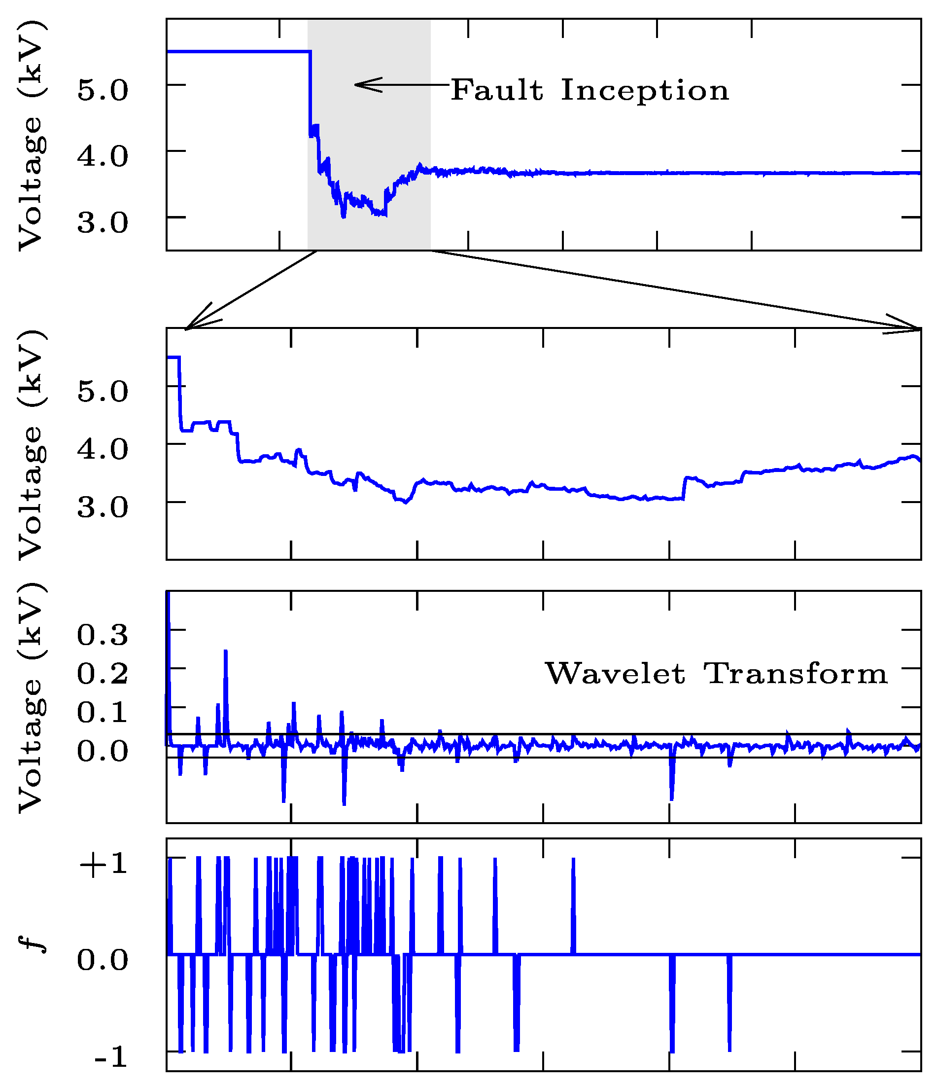
5.1.3. Step 3: Wavelet Transform of Fault Waveform

The post-fault part of the algorithm begins with a recording of the fault waveform at the observation point (the start of the line). To replicate the fault, the EMTP-ATP model of the network is subjected to a single phase to ground fault via a time-controlled switch through an impedance of 10 $\mathsf{\Omega }$ to ground. The observed fault waveform at the observation point is wavelet transformed to convert the discontinuities into a series of sharp pulses, termed f hereafter. Care must be taken in choosing the appropriate wavelet to perform this task; in this case, a 4-level Debauchery (type 1) wavelet has provided the most reliable results, corroborating the findings of other works [19,20].

Prior to the correlation of f with the columns of E, it is important to “align” the start of f such that the arrival of the first fault-induced pulse coincides with the reference line of the matrix E. This can be achieved by checking the index at which f exceeds a set threshold, indicating the location of the first pulse following the fault. In practice, the value of this threshold must be high enough as to avoid “false alarms” due to noise, etc., but low enough such that it reliably detects the first transient, including those originating from high-impedance faults.

5.1.4. Step 4: Perform Correlation of E and f

The correlation function, as described in Equation (1), can now be calculated. This process is performed for faults at nodes 10, 30, 50, 90 and 110, 140, 200 and 240, representing distances (from the observation point) of 10 m, 90 m, 150 m, 270 m, 330 m, 420 m, 600 m, and 720 m, respectively. $t_{max}$, which is the number of timesteps following the first arrived transient to include in the correlation, is set to 400. The square of m is taken and plotted in Figure 6 as a function of node, n. Please note that for clarity of presentation, the metric is normalized such that the maximum $m^2$ equals unity. For all cases, the largest value of $m^2$ is at the faulted point. A relationship is observed between the “sharpness” of the metric at the faulted point and the associated correlation coefficient matrices shown in Figure 5b,d,f. For example, it is predictable that the metric is less sharp and pronounced at an $F_P$ = 200 as compared to, say, an $F_P$ = 50. Importantly, it has been found that the metric is highest at the faulted point for all cases, though there are naturally occurring regions away from the fault point at which the metric is relatively high.

6. Impact of Errors

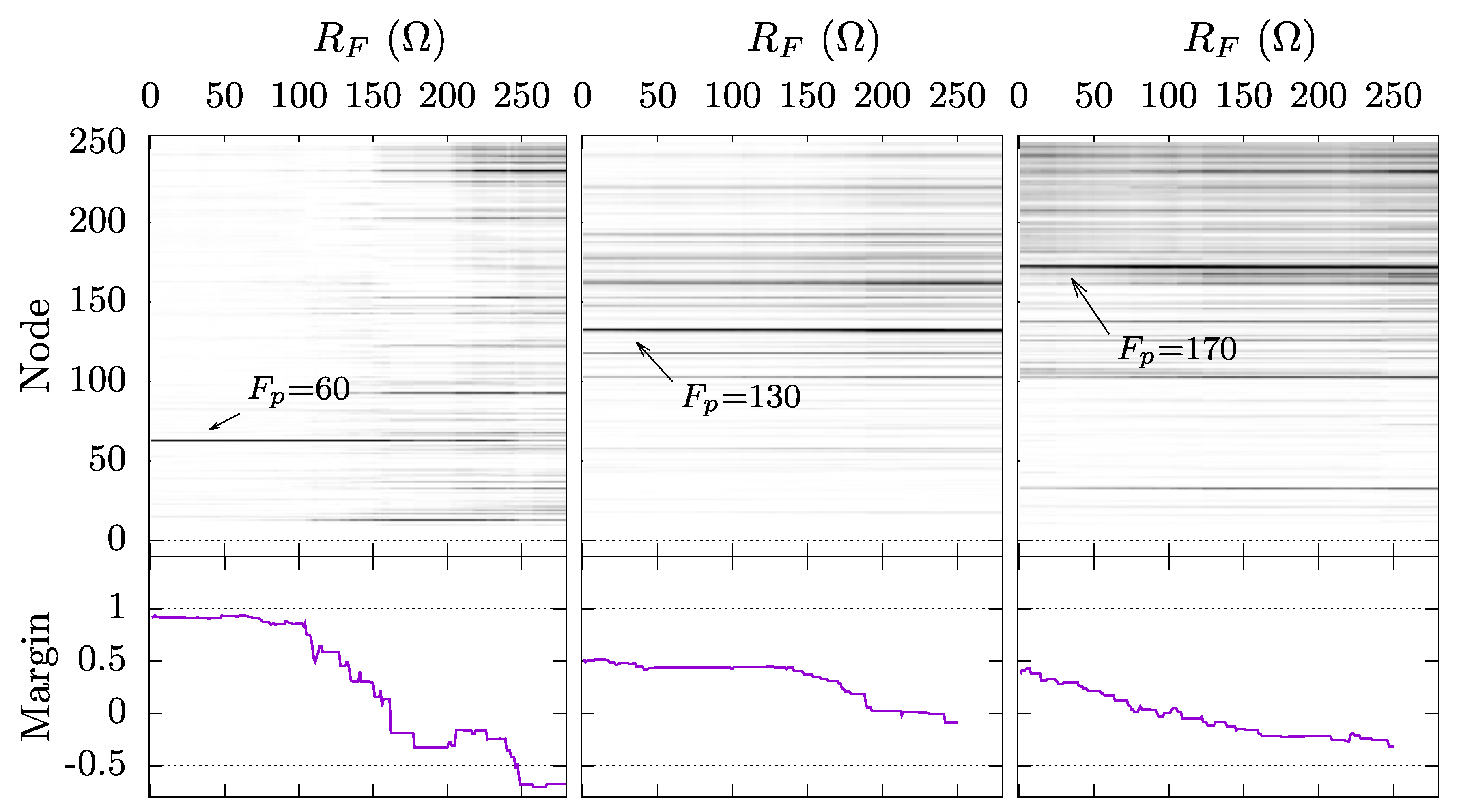
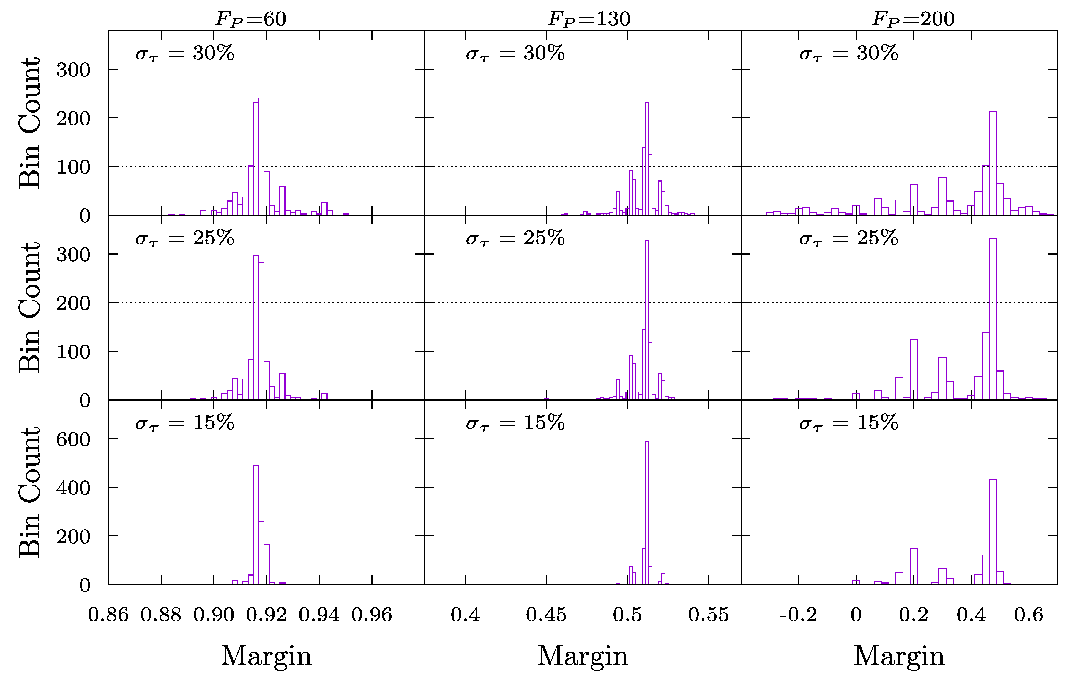
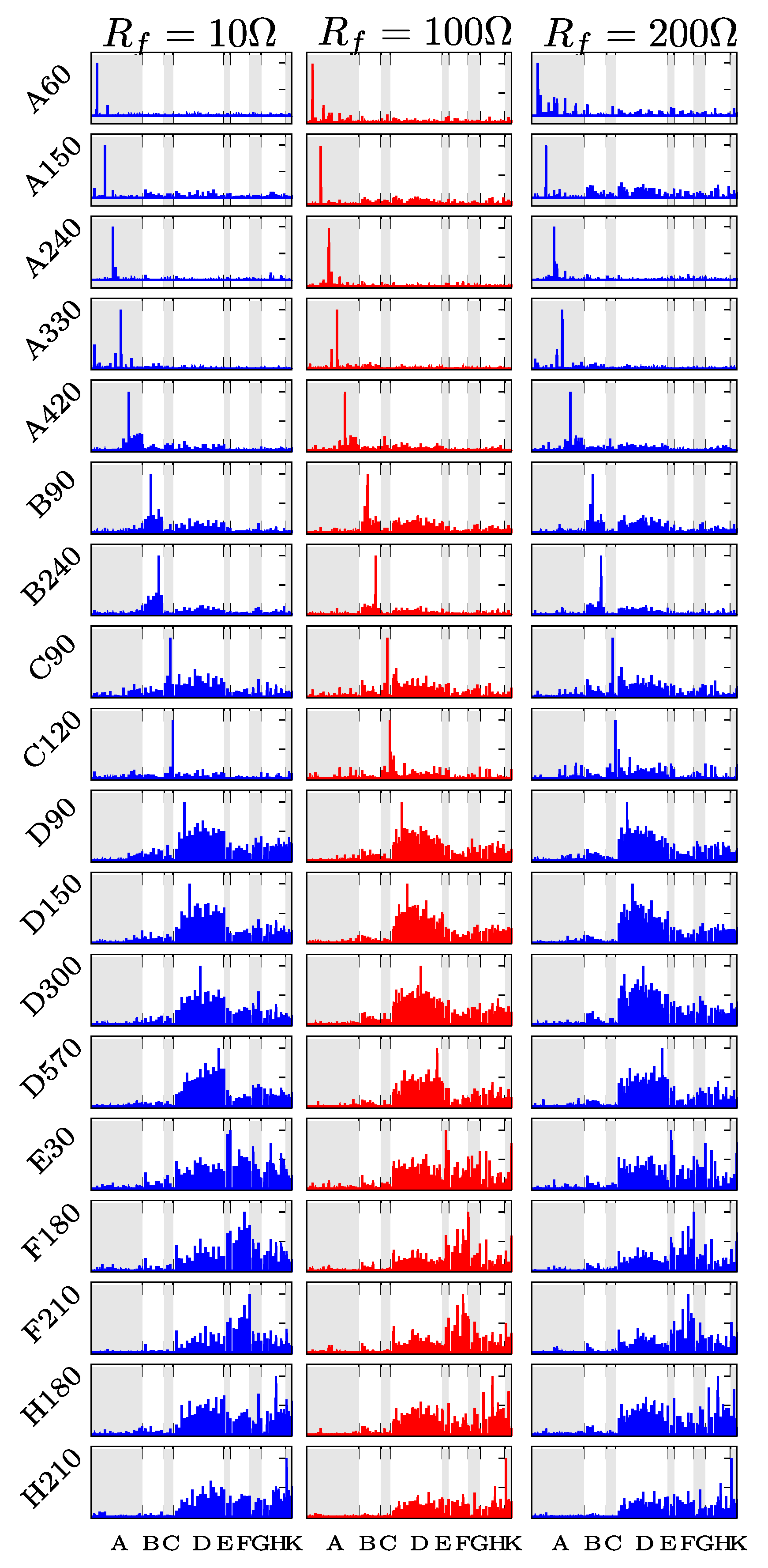
6.1. Effect of Fault Resistance, $R_F$

The fault resistance, $R_F$, is varied between 0 $\mathsf{\Omega }$ and 250 $\mathsf{\Omega }$ in 1 $\mathsf{\Omega }$ increments and at each point the algorithm is carried out based on an E calculated with a 10 $\mathsf{\Omega }$ impedance. This procedure is automated via a MATLAB script which repeatedly calls the EMTP via a DOS command while interactively modifying the ATP file to change $R_F$ between runs. In this example, line 3.2 is used, with the results shown in Figure 7 for three arbitrarily chosen fault locations in the form of heat maps, where the darker shades represent higher values of normalized $m^2$. The “margin”, which is a dimensionless quantity defined as $m^2$ at the fault location divided by the highest $m^2$ across all other nodes, is also plotted as a function of $R_F$. Under these conditions, the margin stays positive (meaning a correct fault-location estimation) until $R_F$ exceeds approximately 150 $\mathsf{\Omega }$. Given that the fault impedance, at that stage dependent on the arc, is likely to vary in the immediate post-fault period, the ability of the algorithm to still operate successfully across a wide range of $R_F$ is a useful attribute. It is observed that successful operation at higher values of actual $R_F$ is possible if E is also calculated with a higher value of $R_F$.

6.2. Effect of Errors in the Magnitude of the Reflection Coefficients

A Monte Carlo approach is used to vary the reflection coefficients in line 3.2 by a standard deviation, $\sigma$, of 30%, 25% and 15%, with 1000 simulation runs per case. Please note that E is calculated using the “correct” value of $\tau$ at each reflection point. Figure 8 shows histograms of the results for three arbitrarily chosen fault locations. In general, the method is resilient against errors in the magnitude of the estimated $\tau$ though fault positions towards the end of the line are more affected than nodes at the start and middle.

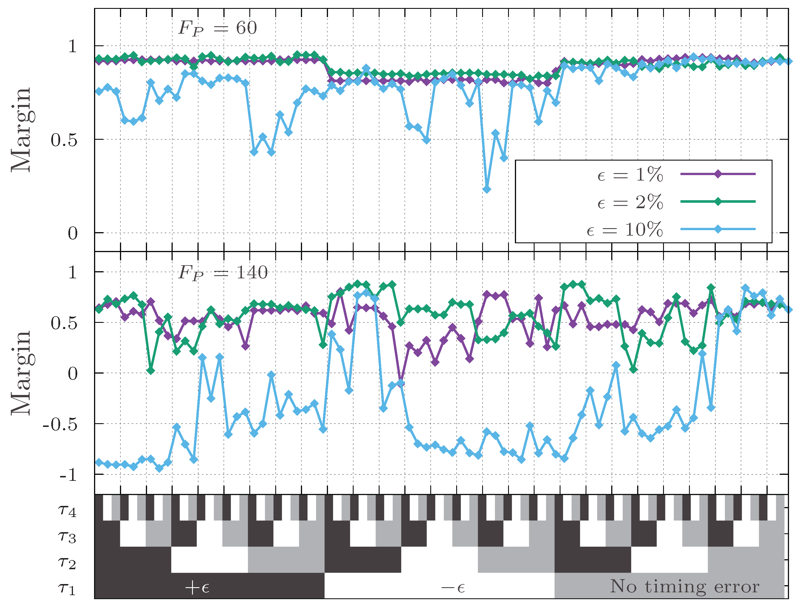
6.3. Robustness Against Timing Errors

The effect of timing error is considered by offsetting the positions of the reflection coefficients both positively (further down the line) and negatively (closer to the source). This process is carried out for line 3.2, with each reflection point offset by a percentage, $ϵ$ of line distance between the neighboring 2 reflection points (or the source and end point). Figure 9 shows the result of this analysis for $ϵ$ = ±1%, ±2% and ±10%, for $F_P$ = 60 and $F_P$ = 140 (chosen as representative of the full range of fault positions). The matrix at the bottom of Figure 9 is color coded to indicate the timing error on each reflection point (black = −$ϵ$, white = +$ϵ$, gray = no timing error). For $F_P$ = 60, the margin is particularly affected by a negative offset at ${\tau }_1$. For $F_P$ = 140, the performance is less robust against timing error, especially for $\left|ϵ\right|=10\%$. In general, fault positions farther away from the source and separated by more reflection points, are more sensitive to timing offsets, though positive margins are still observed for $\left|ϵ\right|$$<$$2\%$.

7. Application of the Proposed Method on the IEEE 13-Bus Network

7.1. Network Modelling

To test the proposed method on a realistic radial network, an adapted form of the IEEE 13-bus network is used. For the purpose of this work, several modifications on the network proposed in [38] have been made:

• All lines are three-phase overhead as detailed in Table 1.
• The voltage regulator and shunt capacitors are omitted.
• Tapped transformers are represented by a lumped resistance of 600 $\mathsf{\Omega }$, and placed arbitrarily around the network at a density approximating 1 transformer per 80 m.

To determine the reflection coefficients, the procedure outlined in Section 3 is performed on each of the branches with an open termination. It must be noted that a similar procedure to determine the reflection coefficients on lines with no open-end termination (i.e., branches E and D, as labelled in Figure 10) is not presented in this work, so these are entered into the line model manually. In practice, these could be estimated based on network information.

Figure 11 shows the raw fault waveform, its wavelet transform, then the “barcode”-like signal f. f is subsequently compared with all columns in the matrix E, where each column represents a prediction of the received f for a particular node in the network. The column of E corresponding to the fault point will give rise to a strong peak when correlated with f, since f and E are derived from the same network.

7.2. General Performance

Figure 12 shows the normalized metric $m^2$ for faults at various positions on the IEEE 13-bus network at a Signal to Noise ratio of 40 dB. The simulations are repeated for fault resistances of $R_f$ = 10 $\mathsf{\Omega }$, 100 $\mathsf{\Omega }$ and 200 $\mathsf{\Omega }$ (where E is calculated based on $R_f$ = 10 $\mathsf{\Omega }$), and with a $t_{max}$ of 400 timesteps (following the arrival of the first fault-induced transient). For all cases, the correct fault location is obtained (“1” represents the maximum correlation). The margin (as defined in Section 6) noticeably decreases the further away the fault position is from the observation point, but robust performance is nevertheless still achieved. The robustness of the proposed method is derived from the fact that high-frequency energy immediately following a fault will arrive at the observation point in particular windows which are defined by the reflection coefficients in the network. Knowing the precise location of the reflection coefficients allows for an accurate prediction of the sequence of high-frequency transients at the observation point.

It is important to note that the proposed method is reliant on there being a distinction (in time) between the arrived high-frequency transients. This will be greatly compromised on larger overhead networks with a high concentration of reflectors or underground cables. However, excellent performance was observed on the IEEE 13-bus network. Further work is required to develop the technique for good performance on larger networks with a greater degree of dispersion and more concentrated reflectors.

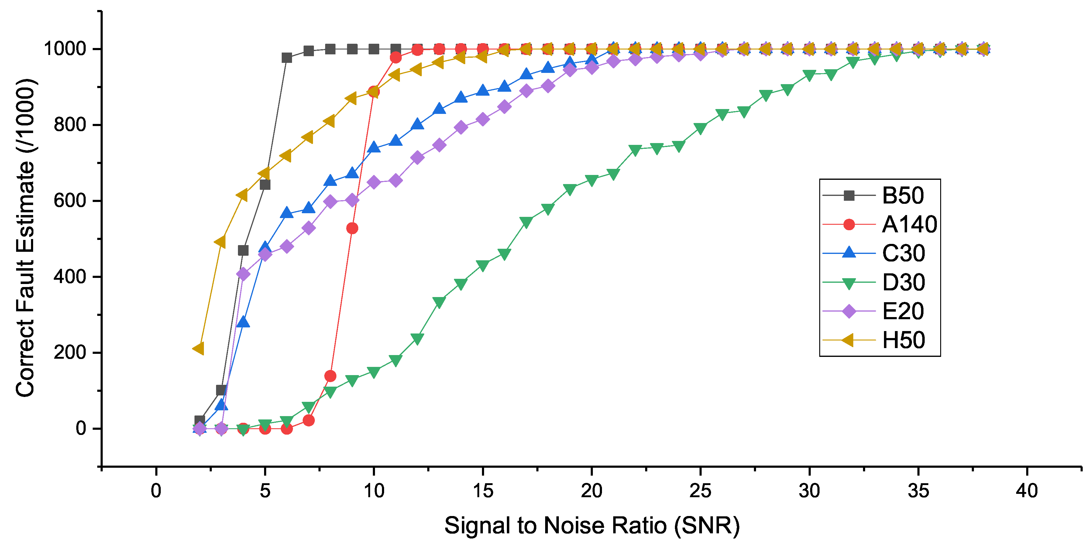
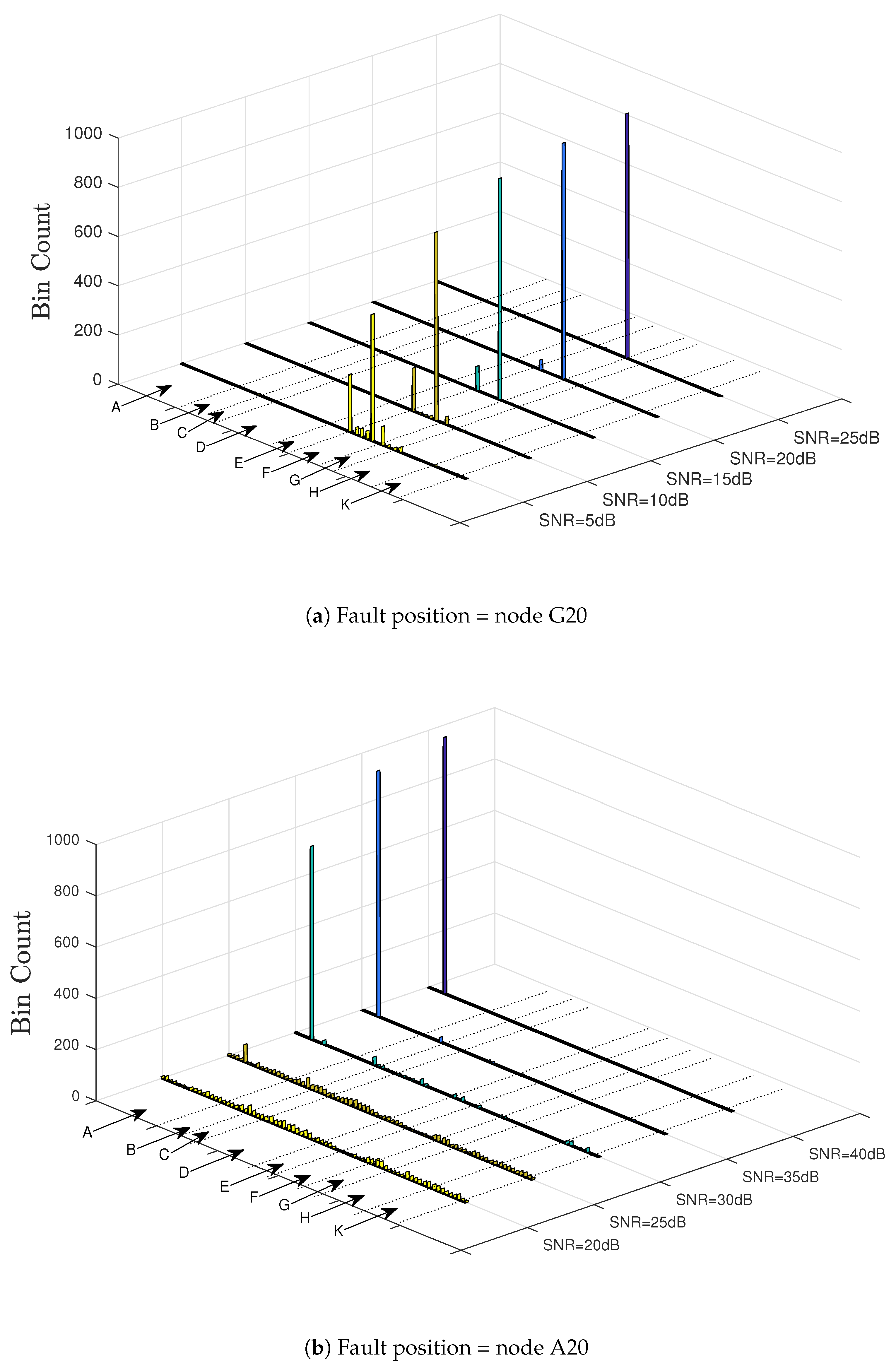
7.3. Performance in the Presence of Noise

To test the performance of the proposed method under the presence the Additive White Gaussian Noise (AWGN), Monte Carlo analyses have been performed for a wide range of SNRs and fault positions. Figure 13 shows SNR versus the proportion of correct fault estimates out of 1000 runs per point. In all cases, 100% accuracy is achieved at an SNR of 35 dB and above. It is particularly noticeable that for some fault positions, the same is achieved for SNRs as low as 5 dB. The inherent robustness to noise is attributable to the fact that energy produced by the fault and observed at the observation point is concentrated at specific intervals of time. It is only necessary for the arrived pulses to rise above the noise floor to be detectable, provided that the threshold value is indeed above the noise floor. This is also demonstrated by considering Figure 14a,b, which shows histograms of estimated fault position for nodes G20 and A20, respectively. For the latter, 100% accuracy is achieved until an SNR of 25 dB, upon which the accuracy drops to close to 0%. For the former, the drop is less abrupt and happens at lower SNRs.

It has been noticed that fault positions exhibiting better SNR performance tend to be those with high magnitude pulses in the opening 200 timesteps following the fault inception. Setting the threshold as a proportion of the magnitude of the first arriving transient, which is likely to be the largest, provides an automatic means to adjust the threshold such that it is low enough to capture smaller later pulses, but high enough to be above the noise floor.

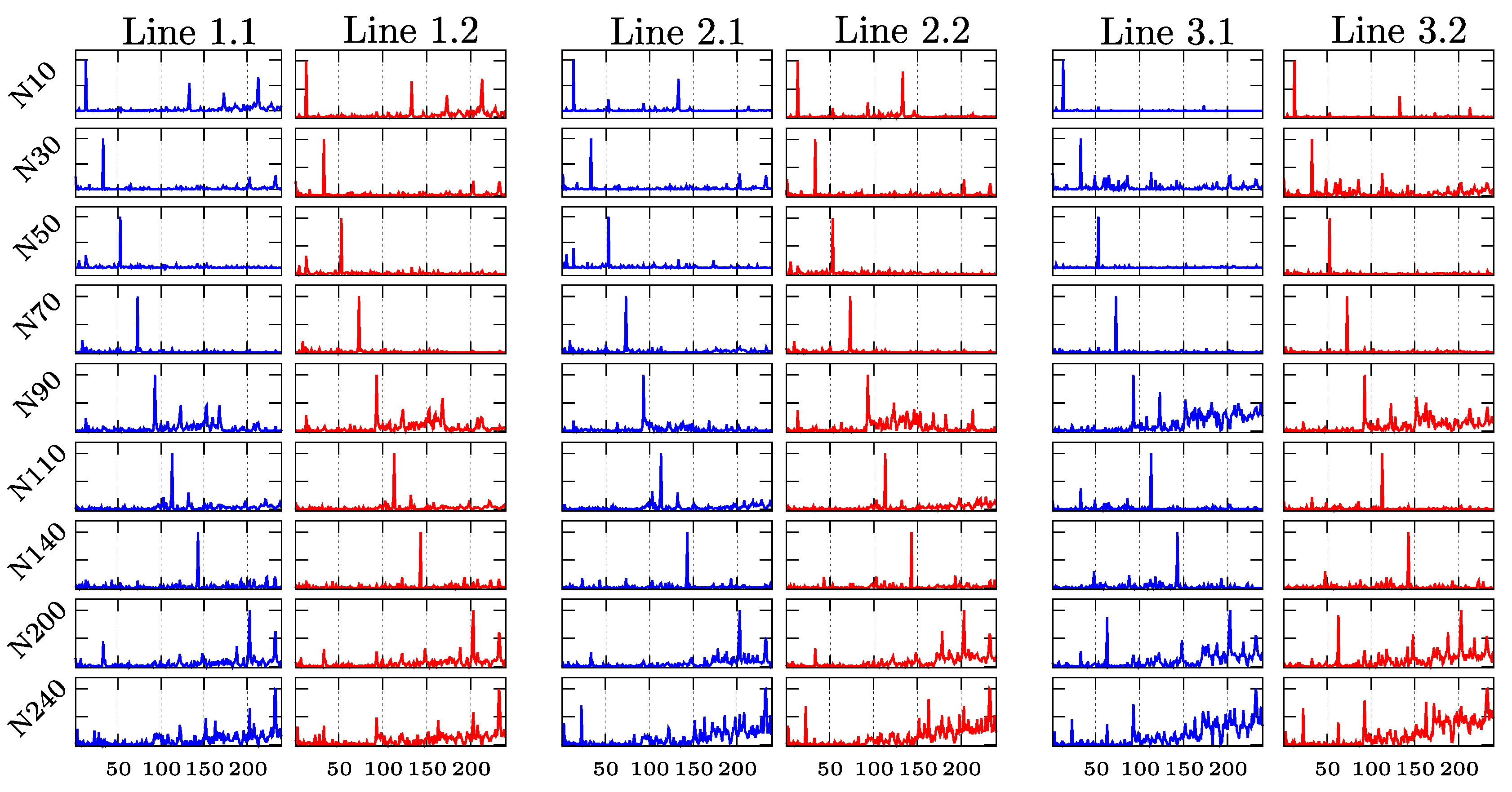
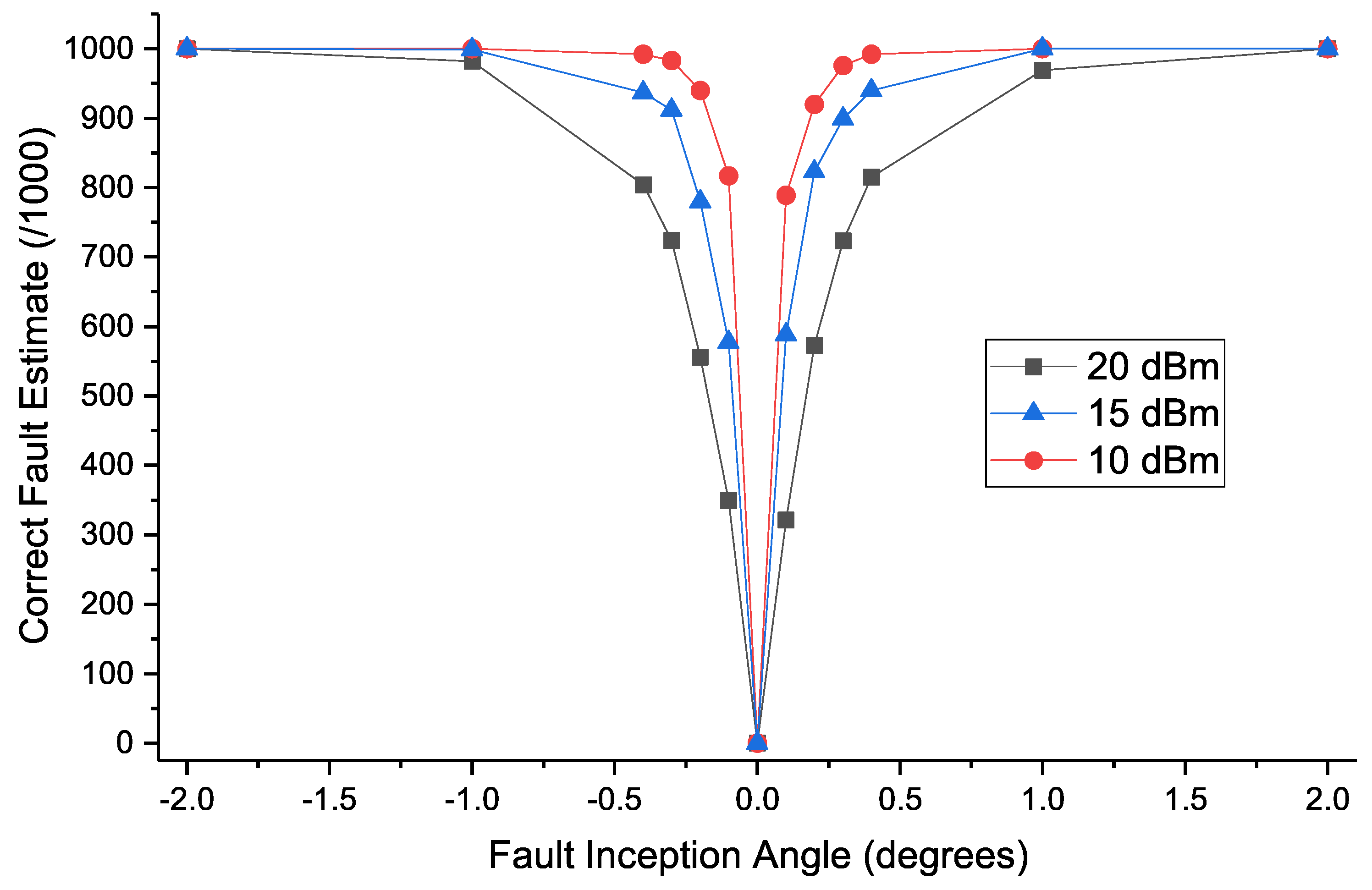
7.4. Effect of Fault Inception Angle

The fault inception angle affects the magnitude of the induced traveling waves. This phenomenon is well covered in [39], which found that for single phase to ground faults (the most common), the peak magnitude occurs at a fault inception angle of $90°$ and the minimum occurs at $0°$. Therefore, at fault inception angles approaching 0°, a breakdown in performance would be expected due to the fault-induced energy at the observation point dropping below the background noise, leading to poor SNRs. Figure 15 reports Monte Carlo simulations using 1000 test runs at different fault inception angles and AWGN noise levels. Please note that the assumption of noise levels are based on both the work of [40], where empirical measurements on the MV network demonstrated noise Power Spectral Densities (PSDs) ranging from −110 dBm/Hz to −75 dBm/Hz up to 2 MHz, and on the work of [41], which uses a conservative estimate of −105 dBm/Hz for the range of frequencies up to 100 MHz. The noise in dBm is given by:

$$P_{dBm}=PS{D}_{dBm/Hz}+10log\left(B{W}_{Hz}\right)$$

(9)

where $P_{dBm}$ is the noise power in dBm, $PS{D}_{dBm/Hz}$ is the PSD in dBm/Hz and ${BW}_{Hz}$ is the bandwidth of the measured signal, in Hz. In the absence of empirical results which show the noise in the power line immediately following a fault, a conservative base PSD of −75 dBm/Hz is chosen. An additional 5, 10, 15 dB of noise is subsequently added to account for the noise figure of the sampling equipment. This gives an effective noise level of 10, 15 and 20 dBm for a sampling frequency of 100 MHz. With these assumptions, Figure 15 shows a clear breakdown in performance as the fault inception angle reaches 0°. The threshold at which the performance begins to deteriorate is, in all three noise scenarios, at a fault inception angle of approximately ±1%. If it is assumed that the probability of fault occurrence is equally distributed across all the cycle and (conservatively) it is assumed that any inception angle within 1% of zero leads to non-detection, this would equate to 1 in 180 faults not being detected due to the magnitude of the induced traveling waves dropping below the threshold required for detection.

8. Practical Considerations

One of the key practical issues with the proposed method relates to application of the layer-peeling procedure, which requires an injection of a steep fronted impulse onto, potentially, a live network. One means of achieving this is via the use of a broadband inductive coupler, which are commonly used to provide high bandwidth (up to 30 MHz) coupling for PLC systems. Another potential means of coupling is use the capacitive divider in the VDS, which was recently proposed [29]. The injection power is likely to be the same magnitude as commonly used in existing PLC networks and suggested by emerging narrowband PLC standards [42]. Using the VDS provides a low-cost and readily available method to both perform the layer-peeling routine and monitor the line for fault activity.

It must be noted that the present method requires the layer-peeling process to be carried out on each line separately, which is time consuming. However, the process is only required to be carried out once to provide instantaneous fault location on branched radial overhead feeders, which are responsible for a disproportionate number of faults on a typical network [1].

On large networks, the proposed method may struggle to differentiate between specific locations due to dispersion, meaning the pulses will tend to smear in time and become indistinguishable. Further investigation of the method is required to determine its performance on, for example, larger distribution or transmission networks. However, on small to medium sized networks, for example the IEEE 13-bus network, good performance was observed, even in the presence of noise. This is due to the strong similarity between the post-fault signal energy at the observation point, and the predicted energy based on actual network measurements.

Future work related to the proposed method will focus on optimization of the feature extraction process and the exploration of domain learning and dimensionality reduction.

9. Conclusions

Many fault-location algorithms rely on a precise simulation model of the real network, but this is difficult to achieve in practice. The method proposed here overcomes this weakness by incorporating a layer-peeling algorithm to recursively determine the reflection coefficients on a line or network. This information is used to construct vectors of “expected” pulses for faults at each position on the network. The correlation of the actual, wavelet transformed fault signal, at a single observation point, with the vectors of expected pulses allows a metric to be formed which maximizes at the position of the fault. EMTP simulations show that the method is capable of detecting faults accurately even if the magnitudes of the reflection coefficients are inaccurate and for timing offset errors <$2\%$ of the distance between reflectors (typically a few meters). This makes the method well suited to practical implementation on complex transmission lines or teed networks.

References

1. Lehtonen, M. Fault rates of different types of medium voltage power lines in different environments. In Proceedings of the 2010 Electric Power Quality and Supply Reliability Conference, Kuressaare, Estonia, 16–18 June 2010; pp. 197–202. [Google Scholar] [CrossRef]
2. Das, S.; Santoso, S.; Gaikwad, A.; Patel, M. Impedance-based fault location in transmission networks: Theory and application. IEEE Access 2014, 2, 537–557. [Google Scholar] [CrossRef]
3. Takagi, T.; Yamakoshi, Y.; Yamaura, M.; Kondow, R.; Matsushima, T. Development of a New Type Fault Locator Using the One-Terminal Voltage and Current Data. IEEE Trans. Power Appar. Syst. 1982, PAS-101, 2892–2898. [Google Scholar] [CrossRef]
4. Zimmerman, K.; Costello, D. Impedance-based fault location experience. In Proceedings of the 58th Annual Conference for Protective Relay Engineers, College Station, TX, USA, 5–7 April 2005; pp. 211–226. [Google Scholar] [CrossRef]
5. Eriksson, L.; Saha, M.M.; Rockefeller, G.D. An Accurate Fault Locator with Compensation For Apparent Reactance In The Fault Resistance Resulting From Remore-End Infeed. IEEE Trans. Power Appar. Syst. 1985, PAS-104, 423–436. [Google Scholar] [CrossRef]
6. Girgis, A.A.; Hart, D.G.; Peterson, W.L. A new fault location technique for two- and three-terminal lines. IEEE Trans. Power Deliv. 1992, 7, 98–107. [Google Scholar] [CrossRef]
7. Personal, E.; García, A.; Parejo, A.; Larios, D.F.; Biscarri, F.; León, C. A Comparison of Impedance-Based Fault Location Methods for Power Underground Distribution Systems. Energies 2016, 9, 1022. [Google Scholar] [CrossRef]
8. Dashti, R.; Salehizadeh, S.M.; Shaker, H.R.; Tahavori, M. Fault Location in Double Circuit Medium Power Distribution Networks Using an Impedance-Based Method. Appl. Sci. 2018, 8, 1034. [Google Scholar] [CrossRef]
9. Krishnathevar, R.; Ngu, E.E. Generalized Impedance-Based Fault Location for Distribution Systems. IEEE Trans. Power Deliv. 2012, 27, 449–451. [Google Scholar] [CrossRef]
10. Salim, R.H.; Resener, M.; Filomena, A.D.; de Oliveira, K.R.C.; Bretas, A.S. Extended Fault-Location Formulation for Power Distribution Systems. IEEE Trans. Power Deliv. 2009, 24, 508–516. [Google Scholar] [CrossRef]
11. Pignati, M.; Zanni, L.; Romano, P.; Cherkaoui, R.; Paolone, M. Fault Detection and Faulted Line Identification in Active Distribution Networks Using Synchrophasors-Based Real-Time State Estimation. IEEE Trans. Power Deliv. 2017, 32, 381–392. [Google Scholar] [CrossRef] [Green Version]
12. Ren, J.; Venkata, S.S.; Sortomme, E. An Accurate Synchrophasor Based Fault Location Method for Emerging Distribution Systems. IEEE Trans. Power Deliv. 2014, 29, 297–298. [Google Scholar] [CrossRef]
13. Crossley, P.A.; McLaren, P.G. Distance Protection Based on Travelling Waves. IEEE Trans. Power Appar. Syst. 1983, PAS-102, 2971–2983. [Google Scholar] [CrossRef]
14. Robson, S.; Haddad, A.; Griffiths, H. Fault Location on Branched Networks Using a Multiended Approach. IEEE Trans. Power Deliv. 2014, 29, 1955–1963. [Google Scholar] [CrossRef]
15. Razzaghi, R.; Lugrin, G.; Manesh, H.; Romero, C.; Paolone, M.; Rachidi, F. An Efficient Method Based on the Electromagnetic Time Reversal to Locate Faults in Power Networks. IEEE Trans. Power Deliv. 2013, 28, 1663–1673. [Google Scholar] [CrossRef] [Green Version]
16. Evrenosoglu, C.Y.; Abur, A. Travelling wave based fault location for teed circuits. IEEE Trans. Power Deliv. 2005, 20, 1115–1121. [Google Scholar] [CrossRef]
17. Magnago, F.H.; Abur, A. Fault location using wavelets. IEEE Trans. Power Deliv. 1998, 13, 1475–1480. [Google Scholar] [CrossRef]
18. Jafarian, P.; Sanaye-Pasand, M. A Traveling-Wave-Based Protection Technique Using Wavelet/PCA Analysis. IEEE Trans. Power Deliv. 2010, 25, 588–599. [Google Scholar] [CrossRef]
19. Kim, C.H.; Kim, H.; Ko, Y.H.; Byun, S.H.; Aggarwal, R.K.; Johns, A.T. A novel fault-detection technique of high-impedance arcing faults in transmission lines using the wavelet transform. IEEE Trans. Power Deliv. 2002, 17, 921–929. [Google Scholar] [CrossRef]
20. Santoso, S.; Powers, E.J.; Grady, W.M.; Hofmann, P. Power quality assessment via wavelet transform analysis. IEEE Trans. Power Deliv. 1996, 11, 924–930. [Google Scholar] [CrossRef]
21. Chen, K.; Huang, C.; He, J. Fault detection, classification and location for transmission lines and distribution systems: A review on the methods. High Volt. 2016, 1, 25–33. [Google Scholar] [CrossRef]
22. Trindade, F.C.L.; Freitas, W.; Vieira, J.C.M. Fault Location in Distribution Systems Based on Smart Feeder Meters. IEEE Trans. Power Deliv. 2014, 29, 251–260. [Google Scholar] [CrossRef]
23. Majidi, M.; Etezadi-Amoli, M.; Fadali, M.S. A Sparse-Data-Driven Approach for Fault Location in Transmission Networks. IEEE Trans. Smart Grid 2017, 8, 548–556. [Google Scholar] [CrossRef]
24. Majidi, M.; Etezadi-Amoli, M. A New Fault Location Technique in Smart Distribution Networks Using Synchronized/Nonsynchronized Measurements. IEEE Trans. Power Deliv. 2018, 33, 1358–1368. [Google Scholar] [CrossRef]
25. Pavlatos, C.; Vita, V.; Dimopoulos, A.C.; Ekonomou, L. Transmission lines’ fault detection using syntactic pattern recognition. Energy Syst. 2018. [Google Scholar] [CrossRef]
26. Mao, X.j.; Qian, J.d. The “peeling” method to process apparent resistivity data for earthquake precursory monitoring. Acta Seismol. Sin. 2001, 14, 685–691. [Google Scholar] [CrossRef]
27. Koltracht, I.; Lancaster, P. Threshold algorithms for the prediction of reflection coefficients in a layered medium. Geophysics 1988, 53, 908–919. [Google Scholar] [CrossRef]
28. Schur, J. Über Potenzreihen, die im Innern des Einheitskreises beschränkt sind. Journal Für Die Reine Und Angewandte Mathematik 1917, 147, 205–232. [Google Scholar]
29. Artale, G.; Cataliotti, A.; Cosentino, V.; Cara, D.D.; Fiorelli, R.; Guaiana, S.; Tinè, G. A New Low Cost Coupling System for Power Line Communication on Medium Voltage Smart Grids. IEEE Trans. Smart Grid 2018, 9, 3321–3329. [Google Scholar] [CrossRef]
30. Yan, F.; Ge, T.-L.; Zhao, H.-S. A New Method of Single-Phase-to-Earth Fault Location for Rural MV Power Networks. In Proceedings of the 2008 Joint International Conference on Power System Technology and IEEE Power India Conference, New Delhi, India, 12–15 October 2008; pp. 1–5. [Google Scholar] [CrossRef]
31. Borghetti, A.; Bosetti, M.; Silvestro, M.D.; Nucci, C.A.; Paolone, M. Continuous-Wavelet Transform for Fault Location in Distribution Power Networks: Definition of Mother Wavelets Inferred From Fault Originated Transients. IEEE Trans. Power Syst. 2008, 23, 380–388. [Google Scholar] [CrossRef] [Green Version]
32. Guzmán, A.; Kasztenny, B.; Tong, Y.; Mynam, M.V. Accurate and economical traveling-wave fault locating without communications. In Proceedings of the 2018 71st Annual Conference for Protective Relay Engineers (CPRE), College Station, TX, USA, 26–29 March 2018; pp. 1–18. [Google Scholar] [CrossRef]
33. Schweitzer, E.O.; Guzmán, A.; Mynam, M.V.; Skendzic, V.; Kasztenny, B.; Marx, S. Locating faults by the traveling waves they launch. In Proceedings of the 2014 67th Annual Conference for Protective Relay Engineers, College Station, TX, USA, 31 March–3 April 2014; pp. 95–110. [Google Scholar] [CrossRef]
34. Wilkinson, W.A.; Cox, M.D. Discrete wavelet analysis of power system transients. IEEE Trans. Power Syst. 1996, 11, 2038–2044. [Google Scholar] [CrossRef]
35. Bruckstein, A.M.; Kailath, T. Inverse Scattering for Discrete Transmission-Line Models. SIAM Rev. 1987, 29, 359–389. [Google Scholar] [CrossRef]
36. Marti, J. Accurate Modelling of Frequency-Dependent Transmission Lines in Electromagnetic Transient Simulations. IEEE Trans. Power Appar. Syst. 1982, PAS-101, 147–157. [Google Scholar] [CrossRef]
37. Snelson, J.K. Propagation of Travelling Waves on Transmission Lines—Frequency Dependent Parameters. IEEE Trans. Power Appar. Syst. 1972, PAS-91, 85–91. [Google Scholar] [CrossRef]
38. Kersting, W.H. Radial distribution test feeders. IEEE Trans. Power Syst. 1991, 6, 975–985. [Google Scholar] [CrossRef]
39. Costa, F.B.; Souza, B.A.; Brito, N.S.D. Effects of the fault inception angle in fault-induced transients. IET Gener. Transm. Distrib. 2012, 6, 463–471. [Google Scholar] [CrossRef]
40. Tao, Z.; Xiaoxian, Y.; Baohui, Z.; Jian, C.; Zhi, Y.; Zhihong, T. Research of Noise Characteristics for 10-kV Medium-Voltage Power Lines. IEEE Trans. Power Deliv. 2007, 22, 142–150. [Google Scholar] [CrossRef]
41. Amirshahi, P.; Kavehrad, M. High-frequency characteristics of overhead multiconductor power lines for broadband communications. IEEE J. Sel. Areas Commun. 2006, 24, 1292–1303. [Google Scholar] [CrossRef]
42. Robson, S.; Haddad, A.; Griffiths, H. A New Methodology for Network Scale Simulation of Emerging Power Line Communication Standards. IEEE Trans. Power Deliv. 2018, 33, 1025–1034. [Google Scholar] [CrossRef]
Figure 1. A pseudofault impulse is injected into the line at 1 m intervals at position r f and a simulation performed to determine the associated response at the source for each injection point. The terminations r s and r t are assumed to be open circuit ( Γ = 1). When the observed signal at the source exceeds a positive threshold, it appears as white, while a signal which is less than a negative threshold appears as black.
Energies 12 00126 g001
Figure 2. MATLAB style code showing the calculation of the backward (left) propagating variable in the impulse response calculation. p is the timestep, n is the node and S is the weighting function.
Energies 12 00126 g002
Figure 3. Overview of the Proposed Algorithm.
Energies 12 00126 g003
Figure 4. Single Line Networks. For the 2-reflector line (a), reflectors are at positions 100 and 180, corresponding to 300 m and 540 m from the start node, respectively.
Energies 12 00126 g004
Figure 5. Expected energy E graphs (left) and their associated autocorrelation functions (right). For the autocorrelations, representing a correlation of +1. Notably, the correlation <1 outside this diagonal.
Energies 12 00126 g005
Figure 6. The metric m 2 computed for faults at different fault positions on the 6 lines detailed in Table 2 and Figure 4. Please note that m 2 is normalized.
Energies 12 00126 g006
Figure 7. Heat Maps of m 2 and Margin ( m 2 (at fault point)/(max m 2 (all other nodes)) as a function of fault impedance R F .
Energies 12 00126 g007
Figure 8. Histograms from Monte Carlo simulations (1000 runs each) showing the distribution of the Margin for σ τ = 30%, 25%, 15%.
Energies 12 00126 g008
Figure 9. Margin as a function of timing error for F P = 60 and F P = 140 of line 3.2. τ 1 , τ 2 , τ 3 and τ 4 are cyclically varied across 3 conditions ( ± ϵ and 0) such that all 81 combinations of timing error are considered. The process is repeated for ϵ = 1%, 2% and 10%.
Energies 12 00126 g009
Figure 10. The IEEE 13-bus network. The network is split into Branches A, B, C, D, E, F, G, H and K. Please note that the distances in the diagram are shown in nodes, where one node is equal to 3 m, e.g., branch A is 600 m long, branch B is 249 m, etc.
Energies 12 00126 g010
Figure 11. Demonstration of the proposed method for node C20 and R f = 10 Ω . The wavelet transformed fault signal is compared to a threshold value and converted into a “barcode”, which is subsequently compared with E to find the highest correlation.
Energies 12 00126 g011
Figure 12. Normalized m 2 for various fault positions on the IEEE 13-bus network at an SNR of 40 dB. The margin is observed to deteriorate as the fault position moves further away from the fault point, but robust performance is still observed. In all cases, the correct fault location coincides with the highest point of the metric.
Energies 12 00126 g012
Figure 13. Signal to Noise Ratio versus the number of correct fault estimates out of 1000 for 6 representative fault positions on the IEEE 13-bus network.
Energies 12 00126 g013
Figure 14. Histograms of estimated fault location versus SNR for two representative fault locations. Each case was run 1000 times at each SNR level. Please note that the two subfigures have different SNR scales.
Energies 12 00126 g014
Figure 15. Correct fault estimates (out of 1000 simulation runs) at difference fault inception angles and noise levels. These tests were performed for a fault location of f p = 140 on the IEEE 13-bus network with R f = 10 Ω and under the conditions described in Section 7.1 and Section 7.2.
Energies 12 00126 g015