Online Calibration Method for Current Sensors Based on GPS

Abstract

At present, most sensor calibration methods are off-line calibration, which not only makes them time-consuming and laborious, but also causes considerable economic losses. Therefore, in this study, an online calibration method of current sensors is proposed to address the abovementioned issues. The principle and framework of online calibration are introduced. One of the calibration indexes is angular difference. In order to accurately verify it, data acquisition must be precisely synchronized. Therefore, a precise synchronous acquisition system based on GPS timing is proposed. The influence of ionosphere on the accuracy of GPS signal is analyzed and a new method for measuring the inherent delay of GPS receiver is proposed. The synchronous acquisition performance of the system is verified by inter-channel synchronization experiment, and the results show that the synchronization of the system is accurate. Lastly, we apply our online calibration method to the current sensor; the experimental results show that the angular difference and ratio difference meet the requirements of the national standard and the accuracy of the online calibration system can be achieved to 0.2 class, demonstrating the effectiveness of the proposed online calibration method.

1. Introduction

In general, any equipment or device that is used to perform measurements should be regularly calibrated. In the same vein, as an important equipment in power systems, a current sensor should be periodically verified to ensure the stability of its current sensor operation as well as the accuracy of its output. This is because a current sensor not only contains components whose performance can degrade over time, including optical and electronic components, but also is often placed outdoors for long time periods [1]. Accuracy and stability of current sensors are important guarantees for measurement, protection, and monitoring of power systems. Periodic verification is a must. Existing current sensor verification technology can be classified into offline verification technology and online verification technology [2]. In particular, offline verification is performed under line power failure conditions, which not only makes the operation complicated, but also affects users in the area served by the sensor, which could lead to considerable economic losses and inconvenience. Therefore, research on online verification technologies for current sensors is particularly significant.

There is much research on the calibration of current sensors. Reference [3] connects two devices by cable, which can realize online calibration. However, it is not suitable for long-distance calibration. If the cable is too long, the current transmission time will be prolonged, which will cause a large time difference. Guo and Crossley [4] presented a procedure to assess the performance of a timing system based on distributed GPS receivers. But this method is expensive and not practical. Liu et al. [5] designed a calibration system based on GPS time synchronization using embedded technology. But its operation is complicated. Furthermore, Vigner and Breuer [6] evaluated the attainable synchronization accuracy within industrial distributed systems. However, the accuracy is not very good.

In order to calibrate the current sensor conveniently and accurately, especially for angular difference calibration. In this study, an online calibration system for current sensors based on GPS timing synchronization is designed. With the increased proliferation of applications using global space positioning, GPS, which can provide all-time-domain, all-weather, high-precision positioning services, has supported extensive changes and far-reaching improvements to various applications [7]. GPS timing can not only improve the accuracy of calibration, but also be applied to the calibration of devices far away from each other.

Before being applied for online calibration of a current sensor, the synchronization accuracy of the proposed system is verified via a synchronism experiment. Then, the proposed system is used to perform online calibration of a current sensor to demonstrate its efficacy. Compared with traditional offline calibration methods, the method proposed in this paper doesn’t need to have power off, which can improve work efficiency and save cost. The experiment results show that the accuracy of the online calibration system can be achieved to 0.2 class.

The remainder of this paper is organized as follows. In Section 2, the related knowledge of online calibration is introduced. In Section 3, the application of GPS timing is introduced; in addition, modeling and analysis of the effect of the ionosphere and GPS receiver on the delay of GPS signals is discussed. Section 4 presents our experiments and experimental results. Section 5 and Section 6 provide discussion and concluding remarks respectively.

2. Related Knowledge of Online Calibration for Current Sensor

Here is a detailed description of online calibration.

2.1. Online Calibration Principle

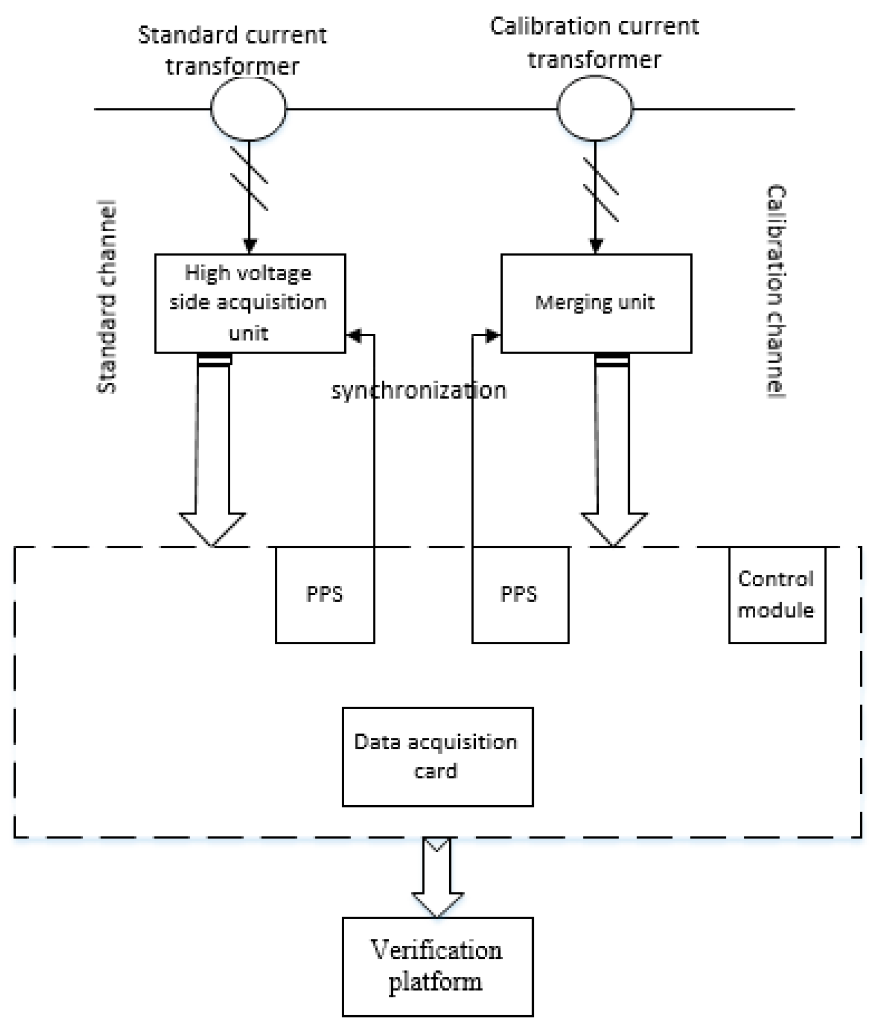
The principle of online calibration of current sensors involves comparing and verifying the digital output of the current sensor being calibrated with the output data of the standard channel on the calibration platform to obtain calibration indexes and their related state quantity under continuous power outage conditions. This principle has been depicted in Figure 1.

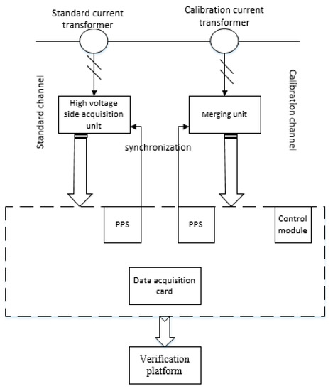
Figure 1. Schematic diagram of the online verification principle for current sensors.

The calibration system is comprised of a standard channel and calibration channel, synchronous control module, data acquisition module, and verification platform. Furthermore, the standard channel consists of a high accuracy standard sensing head, high voltage side current signal acquisition device, optical fiber transmission module, and local receiving module. The calibration channel consists of a calibrated electronic current sensor and merging unit. The merging unit collects data (i.e., current values) from the secondary side of the sensor and converts it into time-based current data output. Lastly, the verification platform includes the frontend computer verification and calibrator software [8].

2.2. Measurement Indicators and Difficulties of Online Calibration

The two primary indexes for current sensor calibration are ratio difference and angular difference [9,10]. Ratio difference is an error value that represents the difference between the actual current sensor ratio and nominal ratio, which are not equal in real-world scenarios. For digital outputs, the ratio difference is expressed as:

$$\mathsf{\epsilon }=\frac{K{I}_S-I_P}{I_P}\times 100\%$$

(1)

where K is nominal transformation ratio, I_P is the root mean square value of the primary current when primary side residual current equals zero and I_S is the root mean square value of the digital output when the sum of secondary side residual output current and secondary side DC output equals zero.

Furthermore, the definition of angle error definition is divided into two, one for analog outputs, and one for digital outputs. For an analog output, the angular difference between the primary and secondary signals at the time of measurement is defined as angle error, whereas for a digital output, the difference between the time at which a current is recorded and the time at which the data is transmitted at the secondary end is defined as so. The electronic current sensor phase difference φ is the difference between the phase of the primary current phasor and secondary output phasor; the phasor direction is selected such that the phase difference angle of the ideal sensor is equal to its rated value at the rated frequency. The phase difference is positive when the secondary output phasor leads the primary current phasor.

In particular, calibration based on angular difference requires the two acquisition equipments being used to be preciously synchronous, otherwise significant errors can occur during calibration. When two acquisition devices that need to be synchronized are not too far apart, they can be synchronized by connecting cables [11]. However, if these two acquisition devices are far apart, this method cannot guarantee accurate synchronization. Because most data acquisition devices are based on the traditional time model, acquisition time may not be accurate due to transmission delay. In particular, the traditional clock model involves a clock frequency generated by a crystal oscillator [12]; nevertheless, as the crystal ages, it can be easily affected by changes in the external environment, which can cause long-term accuracy drifts, resulting in the decline of its timing accuracy. Consequently, this time difference has a considerable impact on angular difference verification during sensor calibration.

The abovementioned problems with the traditional clock model can be avoided by using satellite positioning systems for time synchronization.

3. Research on GPS Timing

The previous section illustrates the necessity of synchronization acquisition using GPS. This section will introduce the principle of GPS timing in detail. The factors that may cause time delay are analyzed from two aspects: the propagation process of GPS signal and the GPS receiver itself. Models and measurement methods are established respectively.

3.1. Principle of GPS Timing

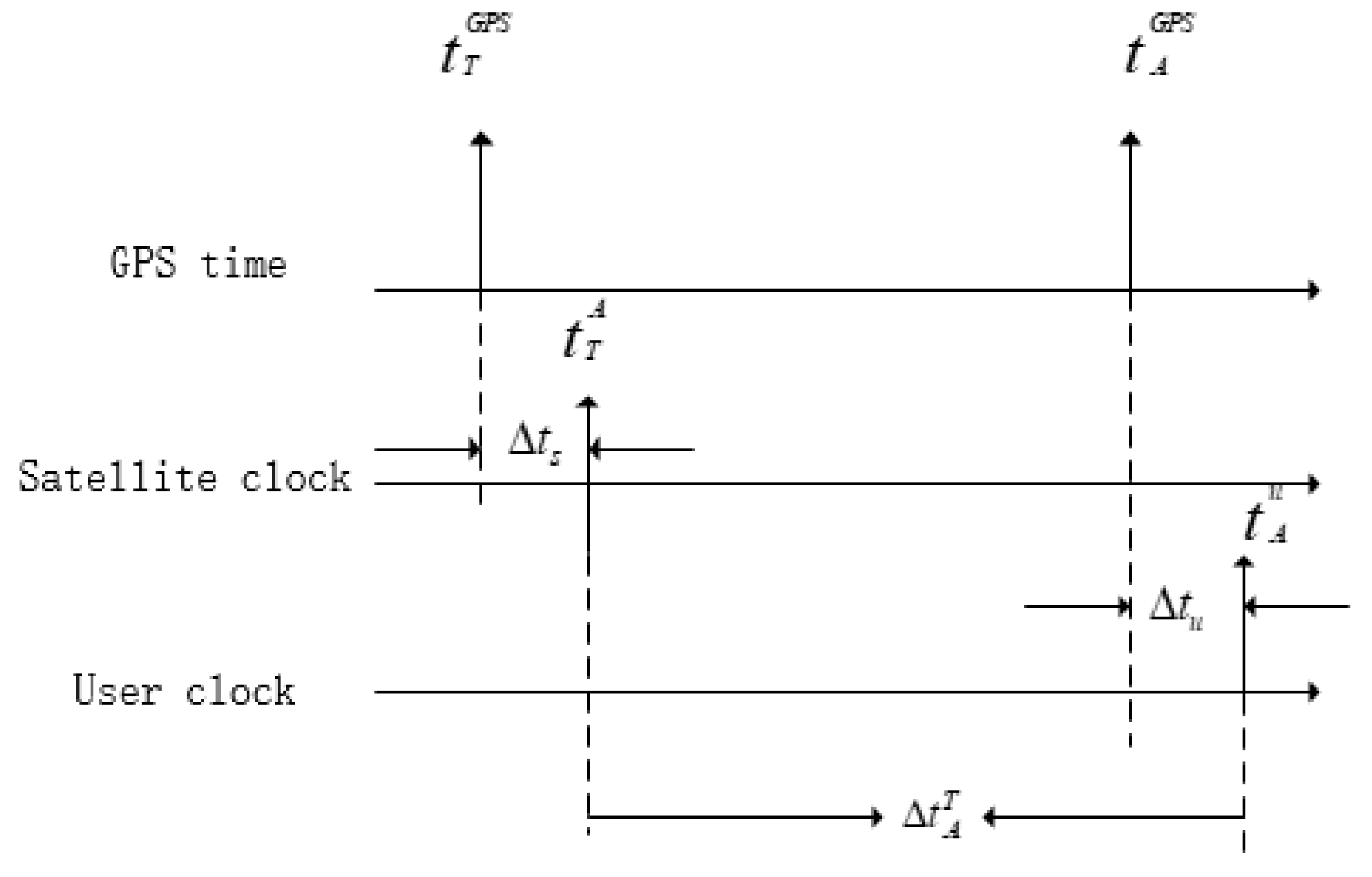
The GPS timing process [13] is shown in Figure 2.

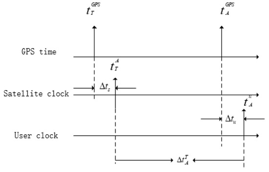
Figure 2. GPS time-transfer process.

The value that each variable specified in Figure 2 signifies is listed in Table 1.

Table 1. Variables used for GPS time-transfer process calculations.

Variable	Value Represented
$t_T^{GPS}$	GPS time when the signal is transmitted.
$t_A^{GPS}$	GPS time according to the user when the signal is received.
$t_A^T$	Satellite clock time when the signal is transmitted.
$t_A^u$	User clock time when the signal is received.
$\Delta t_s$	Deviation between the satellite clock and GPS time.
$\Delta t_u$	Deviation of the user’s clock relative to GPS.
$\Delta t_A^T$	Total propagation time of the signal from the satellite to the user; this can be calculated by the receiver based on the ranging code.

Based on the figure, the following can be deduced:

$$\Delta t_A^T=t_A^u-t_A^T=(t_A^{GPS}-t_T^{GPS})+(\Delta t_u-\Delta t_s)$$

(2)

$$\Delta t_u=\Delta t_A^T-(t_A^{GPS}-t_T^{GPS})+\Delta t_s$$

(3)

Thus, the signal transmission delay based on GPS can be obtained as follows:

$$t_A^{GPS}-t_T^{GPS}={\tau }_R+{\tau }_A+{\tau }_U$$

(4)

In Equation (3), ${\tau }_R$ represents the time delay corresponding to the geometric distance between the satellite and user; it is calculated based on the satellite position and speed of light after the receiver’s position is determined. ${\tau }_A$ represents additional delay introduced by the atmosphere including ionospheric delay and tropospheric delay, which can be calculated using the navigation message. ${\tau }_U$ represents the time delay because of the receiving system, including that caused by the antenna and antenna amps receiver themselves.

From Equations (1)–(3), we can get:

$$\Delta t_u=\Delta t_A^T-{\tau }_R-{\tau }_A-{\tau }_U+\Delta t_s$$

(5)

where $\Delta t_A^T$ can be calculated by the receiver based on the ranging code.

When four GPS satellites are simultaneously observable from the user location, this method can simultaneously measure the user’s clock deviation and station coordinates without prior knowledge of the coordinates of the station [14].

3.2. Time Delay Analysis

According to Equation (5), we will analyze the main factors affecting the accuracy of GPS timing, including ionospheric effect and GPS receiver’s inherent delay.

3.2.1. Ionospheric Effect

In ${\tau }_A$, ionospheric errors have the greatest impact on GPS timing. GPS signals propagate through the ionosphere with a time delay. This is because the ionosphere acts as a scattering medium whose refractive index is a function of the frequency of radio waves owing to the existence of free electrons in it [15,16]. Therefore, we propose a modified ionospheric dual-frequency model to estimate the ionospheric delay. Its schematic graphical representation is shown in Figure 3.

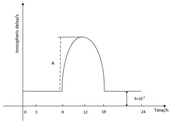
Figure 3. Schematic graphical representation of the ionospheric delay model.

At time t, the ionospheric delay can be expressed as follows:

$$T_r=5\times {10}^{-9}+Acos\frac{2\pi }{P}\left(t-T_P\right)$$

(6)

where A is the amplitude of the cosine function, and it can be calculated as follows:

$$A={\displaystyle \sum }_{n=0}^3{\alpha }_n{\varnothing }_m$$

(7)

Further, P is the period of the cosine function, and it can be calculated as follows:

$$P={\displaystyle \sum }_{n=0}^3{\beta }_n{\varnothing }_m$$

(8)

In Equations (7) and (8), α_n and β_n can be determined based on the navigation message, andΦ_m is geographical latitude of the ionospheric puncture points.

The ionosphere effect could be reduced by 75% when using this model.

3.2.2. GPS Receiver’s Time Delay

As shown in Formula (5) above, ${\tau }_U$ mainly refers to the delay caused by GPS receiver. The host device for a GPS receiver is composed of a frequency converter, signal channel, microprocessor, memory, and display [17], as shown in Figure 4.

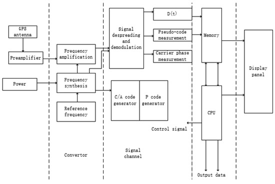
Figure 4. Schematic diagram of the GPS receiver.

The GPS receiver receives the GPS signal via the satellite antenna unit. The pulse per second (PPS) signal outputs through signal filtering, frequency conversion, amplification, and modulus conversion as well as a series of other processing steps. Thus, the inner time delay cannot be ignored. The schematic setup for the absolute calibration of a GPS receiver is shown in Figure 5.

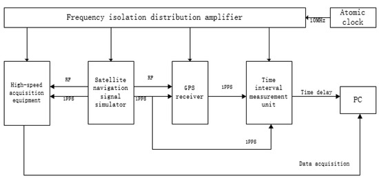
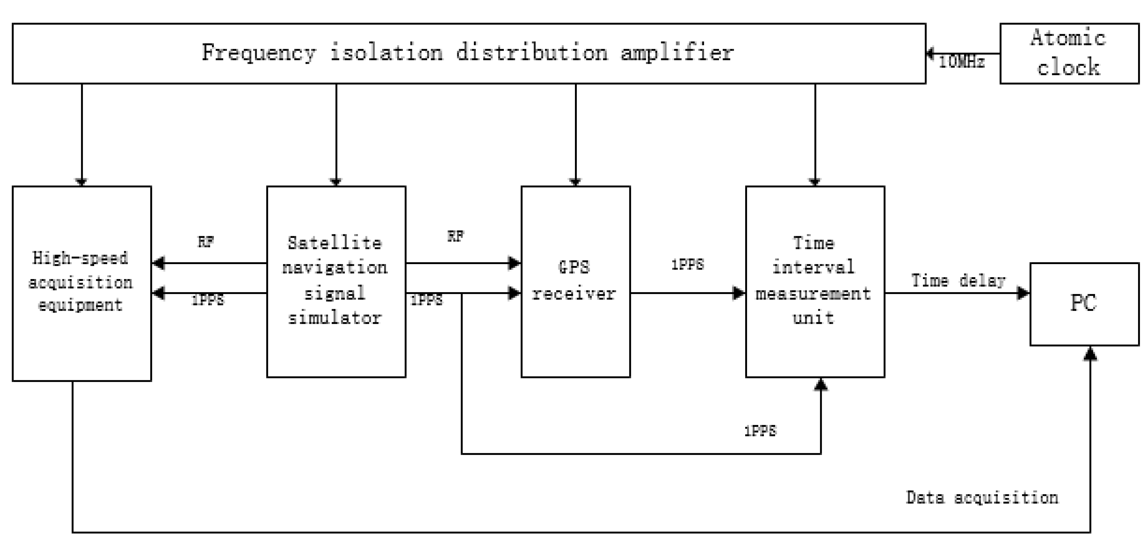
Figure 5. Schematic setup for the absolute calibration of a GPS receiver.

The frequency signal of the local atomic clock provides a unified 10-MHz signal for the calibration system, which is passed through the frequency isolation and distribution amplifier to ensure that the entire calibration system works with the same highly stable frequency standard. After setting the corresponding simulation scene in the satellite navigation signal simulator, it is executed, and the generated satellite navigation RF analog signal and second pulse signal are sent to the high-speed acquisition equipment for data acquisition and storage, following which the collected signal data are sent to the main control computer. Then, the RF analog signal of the simulator and 1PPS are sent to the receiver under test. After the receiver under test has been tracked and positioned normally for a period of time, the internal delay of the receiver can be obtained by comparing the pseudo-range of the receiver’s record with the true range of the simulator’s simulation record [18].

Receiver delay T_r is calculated using Equation (8).

$$T_r+n=\frac{PR-R}{c}-TtC+TtP$$

(9)

where PR is pseudo range and R is true range. n can be considered as Gaussian white noise with a mean of zero; multi-data smoothing can be used to mitigate its impact on calibration.

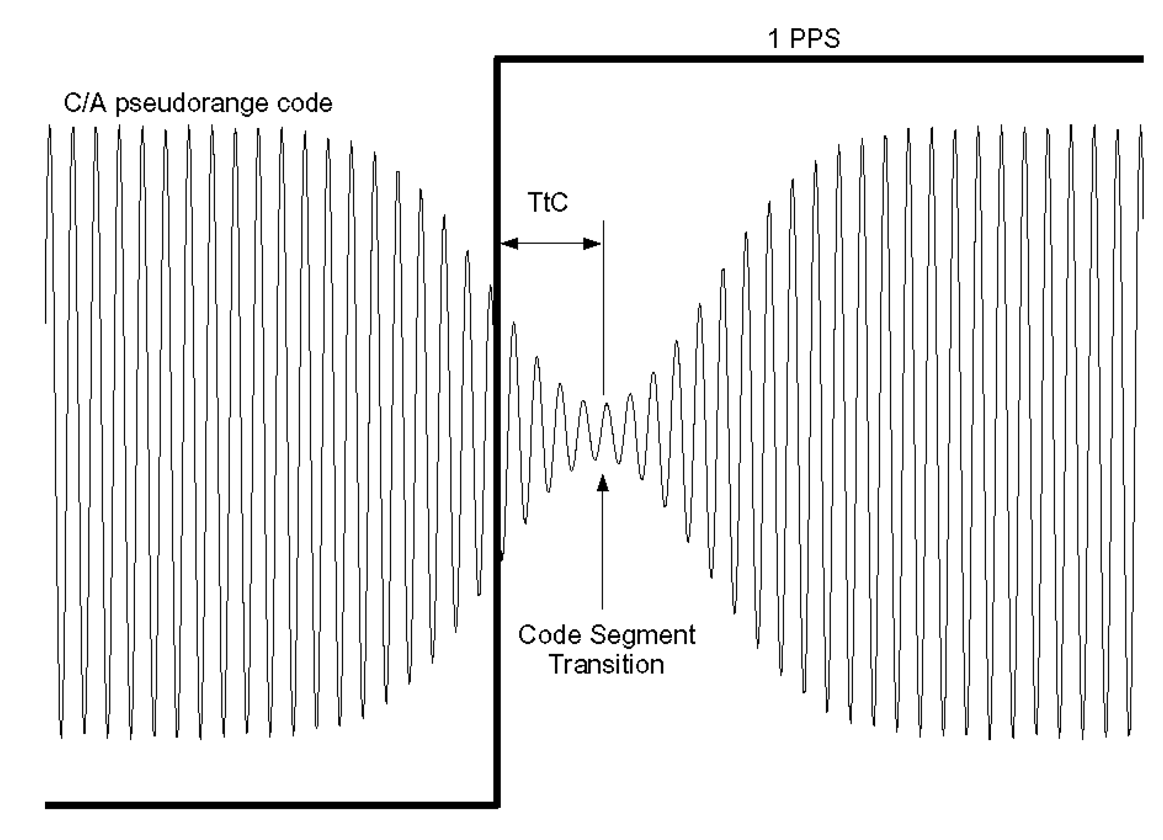
TtC is the difference in the time of arrival between the 1PPS rising edge and pseudo range code transition. The rising 1PPS signal is measured at the point when it achieves 1 V; this is depicted in Figure 6.

Figure 6. Measuring the TtC delay.

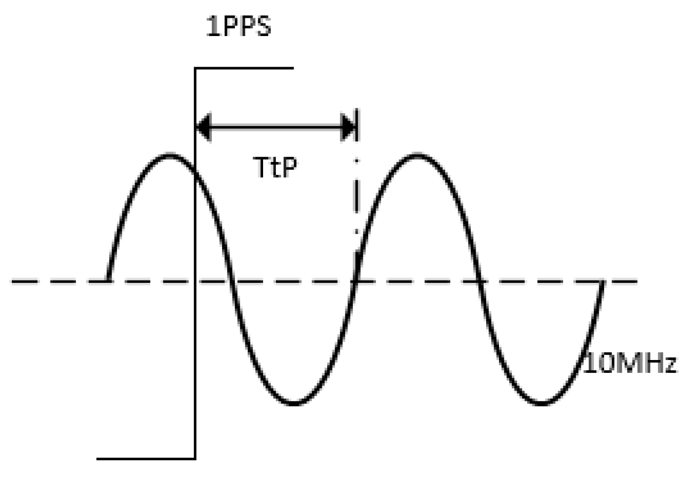
TtP is the time difference between the 1PPS rising edge, and the next rising zero of the 10-MHz clock; this is depicted in Figure 7.

Figure 7. Measuring the TtP delay.

We measured UM220-III L GPS receiver’s inherent time delay at different times, which is shown in Table 2. The average value is within 41 ns, which is about 0.04′ in angle.

Table 2. Inherent time delay of GPS receiver.

Time (h)	Time Delay (ns)
8	40.88
12	41.02
16	41.00
20	40.42
24	40.08

The uncertainty of receiver calibration is mainly caused by antenna, cable, software and measurement repeatability. And it is usually within 2 ns [19,20]. So the inherent delay of the receiver is $\left(41\pm 2\right)$ ns, which is less than 0.05′ in angle. And it is less than 1% of the national standard error and can meet the standard requirements.

4. Experiments

From the aforementioned, we can see the importance of synchronous acquisition in current sensor calibration. Next, we first test the synchronization of the calibration channel and standard channel, and then we conduct online calibration of current sensors.

4.1. Interchannel Synchronization Experiment

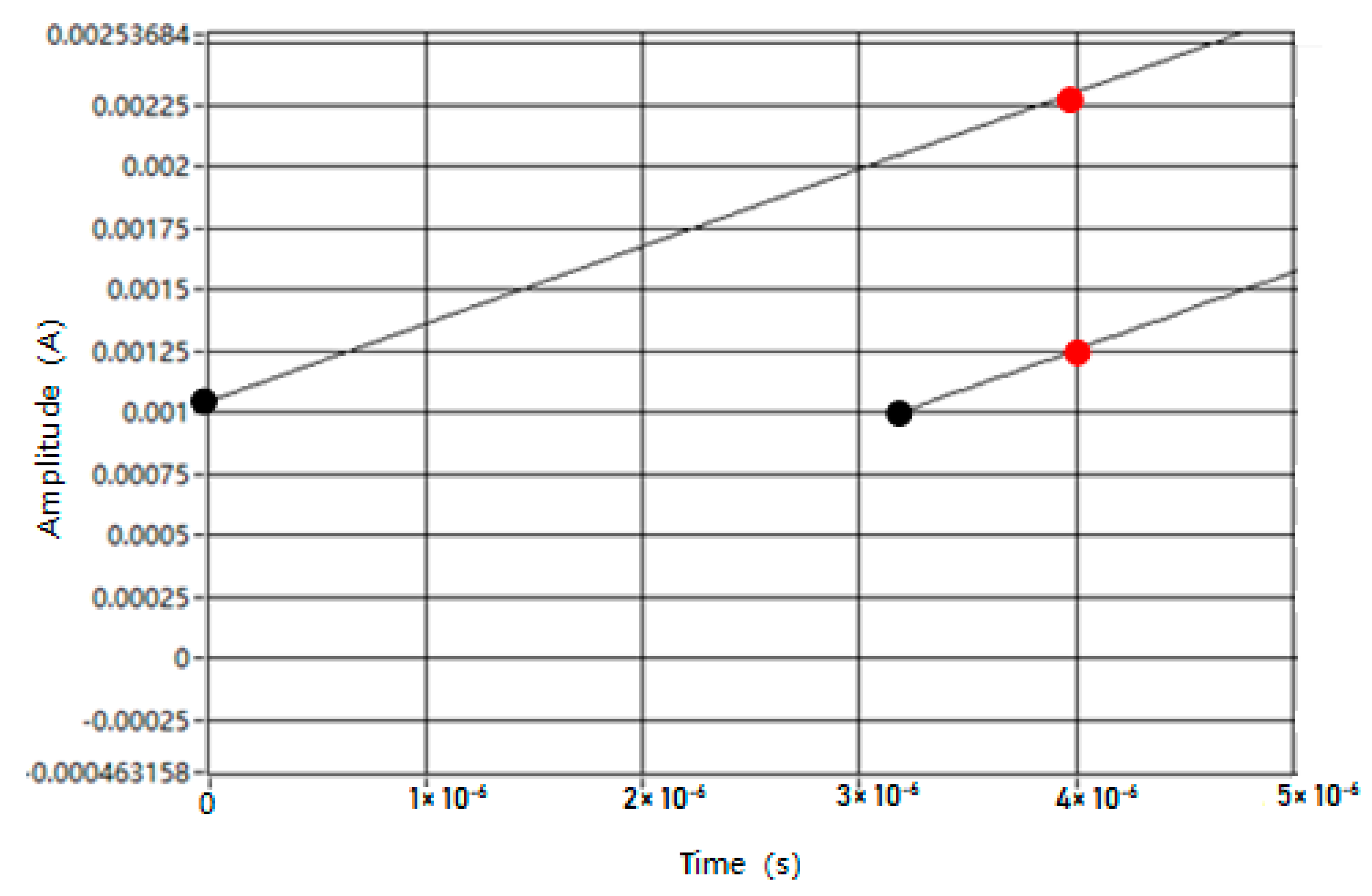
We used a signal generator to generate a sine wave and the frequency is set to 50 Hz (power frequency); the calibration channel and standard channel are used for data acquisition. The waveforms of the two channels are shown in Figure 8. The difference between the abscissa of two black points is angle difference, and the difference between the ordinate of two red points is amplitude difference. The sampling time difference between two channels is close to 3 ns, which is 0.003′ in angle difference, and the amplitude difference is 0.001 A. The synchronization of the two channels is good.

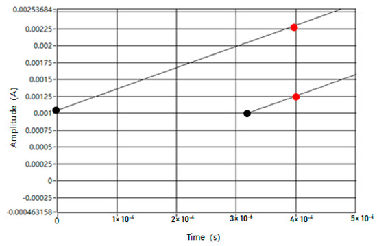
Figure 8. Two-channel waveform used for data acquisition.

In order to verify the influence of power grid frequency fluctuation on the synchronization of the system, we change the frequency of the signal generator and measure the angle difference and amplitude difference between the two channels at 49.5 Hz and 50.5 Hz respectively. The results are shown in Table 3.

Table 3. Difference between two channel signals at different frequencies.

Frequency (Hz)	Angle Difference (′)	Amplitude Difference (A)
49.5	0.005	0.002
50.0	0.003	0.001
50.5	0.004	0.003

Thus, it can be concluded that the two acquisition signals are perfectly synchronized. Even in the case of frequency fluctuation, angle difference is less than 5 ns, which is 0.005′ in angle. It is less than one thousandth of the national standard error. Hence, the acquisition system can achieve accurate synchronous data acquisition.

4.2. Online Calibration of Current Sensor

Through the experiment described above, the synchronism of the data acquisition system was verified. Then, we conducted current sensor online calibration experiment. As previously specified, the primary indicators for sensor calibration include angular difference and ratio difference.

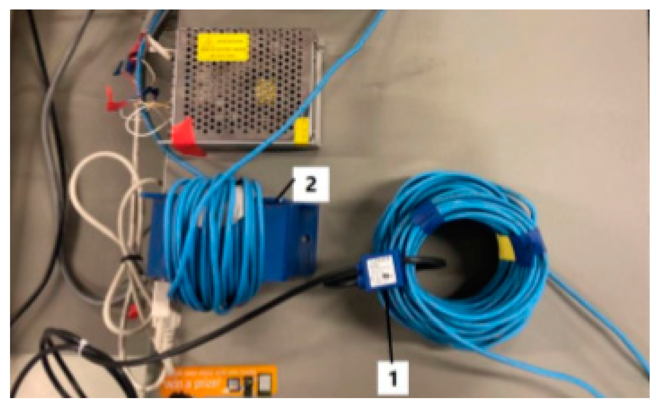
The current sensor to be verified is of 0.2 class, which is marked as 1 in Figure 9; this sensor is an RT500 type sensor that is manufactured by the LEM Company. The sensor marked as 2 is a standard current sensor and is used as a reference for verification; this standard sensor is the ITN1000-S, which is also manufactured by the LEM Company.

Figure 9. Sensor to be calibrated and standard sensor for the experiment.

We adjust the primary input current of current sensor for calibration at 10%, 20%, 40%, 60%, 80%, 100% and 120% of the rated current respectively. 0.2 class national standard error for current sensor calibration are shown in Table 4. The ratio difference and angular difference of each measuring point should not be greater than the data in the table before they meet the national standard.

Table 4. 0.2 class national standard error of ratio difference and angular difference.

Percentage of Rated Current (%)	10	20	40	60	80	100	120
Ratio difference (%)	0.75	0.6	0.2	0.2	0.2	0.2	0.2
Angular difference (′)	25	20	10	10	10	10	10

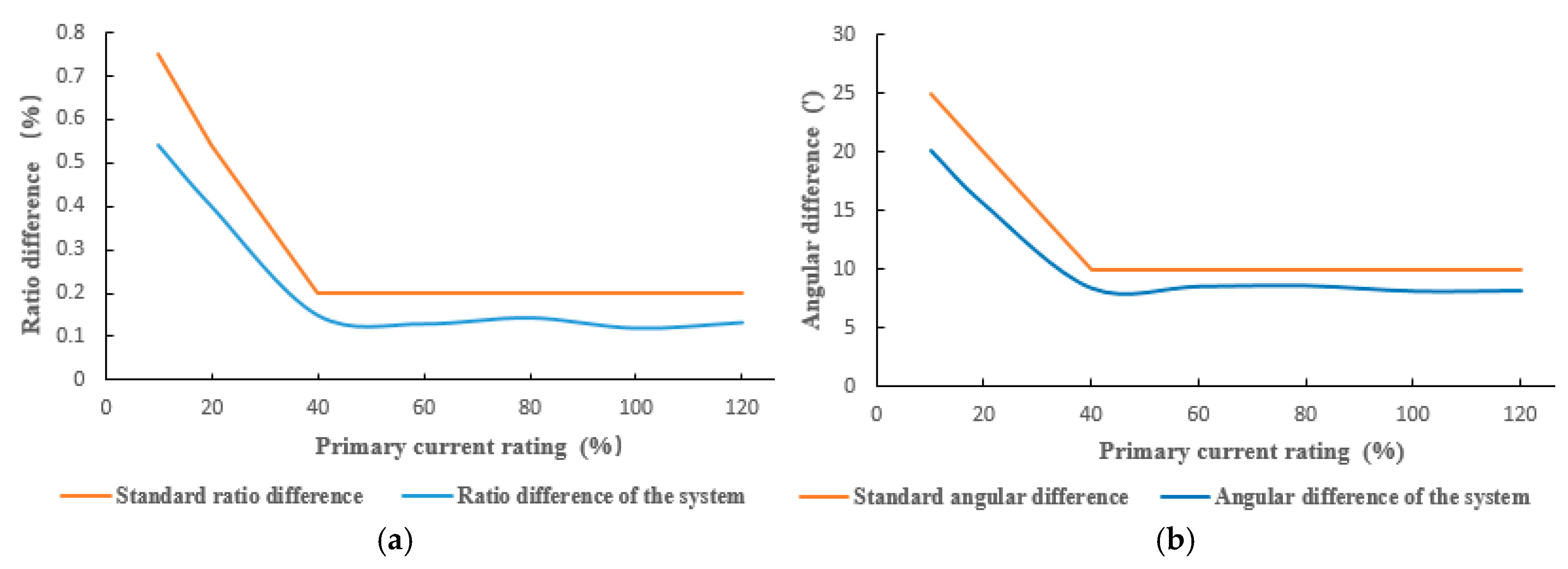
The obtained experimental results are shown in Figure 10. The yellow line is ratio difference and angular difference required by the national standard, and the blue line is the experimental result. It can be seen that the ratio difference is strictly less than the required national standard error value at all measuring points; this is also true in the case of the angular difference. Thus, both the indicators meet the standard requirements of the 0.2 class. Thus, the experimental results confirm the effectiveness of our proposed method, which is of great significance for online calibration of current sensors.

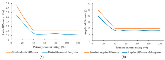
Figure 10. (a) Ratio difference of the system and standard ration difference; (b) Angular difference of the system and standard angular difference.

5. Discussion

Our experimental results indicate that the sensor that is calibrated meets the national standard for ratio and angular differences, and thus, can operate in a normal manner after calibration. However, if this result would not have met the national standard values, the sensor could be broken and should be replaced.

Through our analysis of GPS transmission error and receiver delay, the precision of the proposed synchronous data acquisition system based on GPS timing can attain a value of 0.2 level. The maximum time delay of the calibration system is close to 50 ns. It is about 0.05′ angle difference, less than 1% of the national standard value, which is suitable for most synchronous measurement scenarios. The frequency fluctuation of power grid has little effect on the calibration. The method presented in this paper has high accuracy, strong anti-interference and convenient operation for current sensor calibration.

6. Conclusions

In this study, an online calibration method for current sensors is proposed. In order to check the angle difference accurately, we use GPS timing service instead of traditional timing mode. Per our experimental results, it was demonstrated that the proposed online calibration system achieved good results and can be used to verify current sensors of 0.2 class. Furthermore, its underlying principle can be extended to more applications, especially where accurate synchronous measurements are needed. Moreover, this method and its principle are not only limited to online calibration between two current sensors, but also can be used for online calibration across multiple devices and multiple locations. Thus, our method can serve as a reference for the development and application of GPS technology in other areas of engineering.

References

- Suomalainen, E.P.; Hällström, J.K. Onsite calibration of a current transformer using a rogowski coil. IEEE Trans. Instrum. Meas. 2009, 58, 1054–1058. [Google Scholar] [CrossRef]
- Venikar, P.A.; Ballal, M.S.; Umre, B.S.; Suryawanshi, H.M. A novel offline to online approach to detect transformer interturn fault. IEEE Trans. Power Deliv. 2016, 31, 482–492. [Google Scholar] [CrossRef]
- Shao, M. Research on Online Calibration Method Based on New LVQB Current Transformer. High Volt. Appl. 2016, 8, 45–51. [Google Scholar]
- Guo, H.; Crossley, P. Design of a Time Synchronization System based on GPS and IEEE 1588 for Transmission Substations. IEEE Trans. Power Deliv. 2017, 32, 2091–2100. [Google Scholar] [CrossRef]
- Liu, A.; Li, Z.; Wang, F. Embedded Design of Calibration system based on GPS timing synchronization. EDE 2018, 26, 55–58. [Google Scholar]
- Vigner, V.; Breuer, J. Precise synchronization in large distributed systems. In Proceedings of the IEEE International Conference on Intelligent Data Acquisition and Advanced Computing Systems (IDAACS), Berlin, Germany, 12–14 September 2013. [Google Scholar]
- Ren, X.; Zhang, K.; Li, X. Precise Point Positioning with Multi-constellation Satellite Systems: BeiDou, Galileo, GLONASS, GPS. Acta Geod. Cartogr. Sin. 2015, 44, 1307–1313. [Google Scholar]
- Slomovitz, D.; Santos, A. On-line calibration of high voltage current sensors. In Proceedings of the Conference on Precision Electromagnetic Measurements Digest, Broomfield, CO, USA, 8–13 June 2008. [Google Scholar]
- Wang, Y.; Sun, J. Research on a method and mechanism of ocean current sensor calibration. Adv. Mater. Res. 2011, 291–294, 2799–2804. [Google Scholar] [CrossRef]
- Lu, D. Test methods and requirements of current sensor ratio difference and angle difference. Sci. Technol. Innov. 2015, 15, 7. [Google Scholar]
- Auler, L.F.; Amore, R. Remote Power Lines Oscillography with High Accurate Time Synchronization. In Proceedings of the International Conference on Advanced Engineering Computing and Applications in Sciences (ICAECA), Papeete, France, 12 December 2007. [Google Scholar]
- Chan, S.C.; Shepard, K.L.; Restle, P.J. Distributed Differential Oscillators for Global Clock Networks. IEEE J. Solid-State Circuits 2006, 41, 2083–2094. [Google Scholar] [CrossRef]
- Myrick, W.L.; Goldstein, J.S.; Zoltowski, M.D. Low complexity anti-jam space-time processing for GPS. In Proceedings of the IEEE International Conference on Acoustics, Salt Lake City, UT, USA, 7–11 May 2001. [Google Scholar]
- Vieira, D. Navigation and Attitude Estimation from GPS Pseudorange, Carrier Phase and dopples Observables. In Proceedings of the 34th COSPAR Scientific Assembly, Houston, TX, USA, 10–19 October 2002. [Google Scholar]
- Krypiakgregorczyk, A.; Wielgosz, P.; Borkowski, A. Ionosphere Model for European Region Based on Multi-GNSS Data and TPS Interpolation. Remote Sens. 2017, 9, 1221. [Google Scholar] [CrossRef]
- Rajesh, P.K.; Lin, C.; Chen, C.H. Global equatorial plasma bubble growth rates using ionosphere data assimilation. J. Geophys. Res. 2017, 122, 3777–3787. [Google Scholar] [CrossRef]
- Wei, Z.; Ke, Z.; Bin, W.B. Simulation and Analysis of GPS Software Receiver. In Proceedings of the IEEE International Conference on Computer Modeling and Simulation, Sanya, China, 22–24 January 2010. [Google Scholar]
- Aparicio, J.M.; Laroche, S. Estimation of the Added Value of the Absolute Calibration of GPS Radio Occultation Data for Numerical Weather Prediction. MWR 2015, 143, 1259–1274. [Google Scholar] [CrossRef]
- Grunert, U.; Tholert, S.; Denks, H. Using of Sprient GPS/Galileo HW Simulator for Timing Receiver Calibration. In Proceedings of the IEEE/ION Position, Location and Navigation Symposium, Monterey, CA, USA, 5–8 May 2008; pp. 77–81. [Google Scholar]
- Jiao, Y. Receiver Delay Absolute Calibration Technology Based on GPS Hardware Simulator. In Proceedings of the 6th Annual Conference of China Satellite Navigation, Xi’an, China, 21–23 May 2015. [Google Scholar]
© 2019 by the authors. Licensee MDPI, Basel, Switzerland. This article is an open access article distributed under the terms and conditions of the Creative Commons Attribution (CC BY) license (http://creativecommons.org/licenses/by/4.0/).