Abstract
Although the size of the wind turbine has become larger to improve the economic feasibility of wind power generation, whether increases in rotor diameter and hub height always lead to the optimization of energy cost remains to be seen. This paper proposes an algorithm that calculates the optimized hub height to minimize the cost of energy (COE) using the regional wind profile database. The optimized hub height was determined by identifying the minimum COE after calculating the annual energy production (AEP) and cost increase, according to hub height increase, by using the wind profiles of the wind resource map in South Korea and drawing the COE curve. The optimized hub altitude was calculated as 75~80 m in the inland plain but as 60~70 m in onshore or mountain sites, where the wind profile at the lower layer from the hub height showed relatively strong wind speed than that in inland plain. The AEP loss due to the decrease in hub height was compensated for by increasing the rotor diameter, in which case COE also decreased in the entire region of South Korea. The proposed algorithm of identifying the optimized hub height is expected to serve as a good guideline when determining the hub height according to different geographic regions.
1. Introduction
As two of the core factors in wind turbine design, hub height (HH) and rotor diameter (RD) have significant impact on power output and facility cost, thereby determining the cost of energy (COE) [1]. Theoretically, as HH increases, wind speed increases. Likewise, longer RD means that the area absorbing wind momentum increases, thereby increasing power output [2]. The effect of surface roughness diminishes with height, so wind speed increment occurs within a mixed layer and mitigates as the height approaches the boundary layer height. Since the overall cost increases with the increase in HH, however, the optimal hub height (OHH) that ensures minimum COE should be at a certain HH for investment efficiency.
Wind power projects aim to minimize capital expenditure (CAPEX) and operation expenditure (OPEX), and to maximize annual energy production (AEP) as with other profit-oriented projects. In other words, the goal of a wind farm design is to minimize COE as a function of CAPEX, OPEX, and AEP, and various studies have been conducted to reduce COE by minimizing wake loss through the optimization of wind turbine layout in a large wind farm [3,4,5,6]. Studies have also been conducted to determine the optimal HH and RD, as the control of HH and RD is more influential in reducing COE than optimizing the layout in a small wind farm.
Lee et al. [7] calculated OHH to maximize the power generation profit, but it was excessively high (150~220 m). They also calculated profit according to the electricity price, so OHH could change if the electricity price or government incentive policy changed. Rehman et al. [8] presumed OHH to be an intersection where the total cost function of HH and a gradient curve of the AEP function were crossed, but they did not present sufficient rationale that the calculated intersection was theoretically OHH, rather they applied their own method to regions with a few observation data. Maki et al. [9] and Mirghaed et al. [10] calculated the minimized COE iteratively with regard to all cases by controlling a variety of variables, including generator’s revolutions per minute (RPM) and turbine pitch, in addition to HH and RD. This was not only complicated, but also incurred high calculation cost. Moreover, these studies do not guarantee a reliable AEP because they used constant wind speed and shear exponent, which hardly makes COE credible for the specific site. Since, Stanley et al. [11] used a gradient-based method, which was also iterative to calculate the optimum value, and it remained site-specific (one site).
In sum, the technical problems of the previous studies were: (1) Variability of OHH due to external factors (government policy or electricity price, etc.); (2) cases that were limited to a few regions only, and; (3) complicated calculations that take a long time as a large number of variables were considered, so it was hard to calculate OHH for a large area.
To overcome the aforementioned problems and limitations of the previous studies, this paper proposes a method that generates the COE curve according to HH, and searches OHH that minimizes COE. This method has nothing to do with government policies and external factors, such as incentive programs or electricity price, and the calculated OHH is dependent only on AEP and COE according to the characteristics of wind resources in the target region. In other words, since all cost information are summed and dealt with as a single variable, OHH can be calculated with fewer computations than other methods that consider a number of variables. This study not only calculated the COE curve accurately using the wind resource map provided by the Korea Institute of Energy Research (KIER), which re-distributed AEP into a 1 km horizontal and 10 m vertical distance grid, but also observed a correlation between OHH and geographical characteristics spatially. In other words, the proposed method can identify the pattern of OHH according to geographical characteristics, such as coast, inland, or mountain regions in South Korea, through the mapping of OHH [12]. Note that this study was limited to onshore wind turbines since the cost information of offshore wind turbines was not as sufficient as that of onshore.
The proposed method produced OHH that was lower than 80 m as the general hub height (GHH) of MW-capacity wind turbines in high wind sites. This may degrade AEP. If sufficient power production is one of the critical goals of the wind power project, it is necessary to have a measure for compensating for the degraded AEP due to the calculated OHH. This study proposed a measure for compensating for the AEP loss by increasing RD. Specifically, the power generation loss due to OHH was compensated for by increasing RD, but COE did not increase even with such compensation.
2. Data and Methods
The following procedure determines the OHH proposed in this study:
- (1)
- Step to prepare wind profile data
- (a)
- The time-series wind profile data are fetched from the grid points in the wind resource map.
- (2)
- Steps to calculate OHH
- (a)
- AEPs are calculated by increasing HH from 40 m to 100 m with 10 m increments.
- (b)
- The COE curve is produced through regression analysis with the calculated AEPs and cost data.
- (c)
- OHH is searched when the COE curve is minimum using a numerical analysis method.
- (3)
- Steps to calculate RD
- (a)
- The AEP loss is calculated when GHH is changed to OHH.
- (b)
- The AEP increase is calculated by raising RD to 70 m, 80 m, 90 m, and 97 m.
- (c)
- The RD that can compensate for the AEP loss due to OHH is determined.
The procedure above is performed with regard to the entire onshore in South Korea.
2.1. Wind Resource Map
As a high-resolution wind resource map produced by KIER, KIER-WindMap was used to employ the time-series data of the wind profile, which were needed to calculate AEP per region. KIER-WindMap was produced by Weather Research and Forecasting (WRF) v3.7.1, a mesoscale numerical weather prediction model. Table 1 presents the configuration of the model in detail. For the initial and boundary conditions, the Regional Data Assimilation and Prediction System (RDAPS), a regional model of 12 km spatial resolution produced by the Korea Meteorological Administration (KMA), was used. The final domain was discretized as a 933 (east-west) × 1332 (south-north) grid, having 1 km × 1 km spatial resolution in a horizontal plane covering the Korean Peninsula (Figure 1), and the vertical layer consisted of 37 layers. The lower layer where the wind turbine is to be located was re-distributed with 10 m interval. The Mellor-Yamada-Janjic scheme was used as the planetary boundary layer parameterization scheme, and the WRF single moment 3-class ice scheme was used as cloud microphysics parameterization [13,14]. The land surface model calculated the physical process of the surface boundary layer (SBL) using the WRF-combined Noah-MP land surface model [15]. To improve the accuracy of KIER-WindMap, observation data (AWS/ASOS, Sonde/Wind profiler, Buoy) of KMA and related institutions were assimilated into the background field using the four-dimensional data assimilation technique. The accuracy of the final wind resource map was proven through various verification studies [16,17].

Table 1.
Model configuration of Weather Research and Forecasting (WRF).
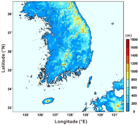
Figure 1.
Terrain elevation of the analysis domain (South Korea).
2.2. COE Curve as a Function of HH
OHH in this study refers to a height that produces the minimum value of COE, which is calculated by dividing the total investment cost (TIC) in a year (Equation (1)) by AEP (Equation (2)). Since coefficient of the highest order term in the COE function (Equation (3)) is larger than zero, it has a convex curve shape in the downward direction (Figure 2). In the condition of , the COE function has minimum value , and is calculated as OHH. In other words, OHH is understood to be a value wherein the derivative of the COE function is 0 (). Using the polynomial regression equations shown in Equations (1)–(3), the downward convex shape of the COE curve can be clearly expressed mathematically. Therefore, the point of OHH where the derivative of the COE curve becomes 0. The and in Equation (2) and in Equation (3) are coefficients that are changed depending on the region, with the coefficients in Equation (1) as constants: . The coefficients of polynomial regression equations are determined using a least square method.
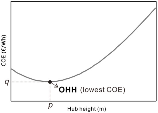
Figure 2.
Cost of energy (COE) curve as a function of hub height hub height (HH). OHH, optimal hub height.
To find OHH, the COE equation is calculated first. AEP and TIC are calculated by changing a 10-m-long HH with 1 m increments through polynomial regression to produce a smooth COE curve. AEP is calculated using the wind turbine performance curve and time-series wind profile data provided by the wind resource map database KIER-WindMap. The South Korea-made STX72-2.0 MW was used as the reference wind turbine, and the rotor equivalent wind speed (REWS) was applied to reflect the characteristics of the regional wind profile correctly (Equation (4)). For the TIC for one year, the cost increase data according to HH proposed in a previous study was used [8]. In other words, it was a divided cost for over one year with regard to the facility cost, construction cost, and maintenance cost across the 20-year service life of the wind turbine.
REWS, which was used instead of HH wind speed in order to avoid overestimating AEP and to consider the regional wind speed characteristics, was calculated by dividing the rotor area by 5 as shown in Figure 3 and area-weighting the wind speed at mid-height of each segment [18,19,20].
where refers to the wind speed at the i-th segment center, is a rotor area, and refers to the i-th segment area.
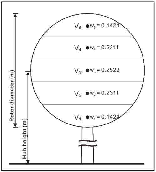
Figure 3.
Rotor area fraction and corresponding weights for rotor equivalent wind speed (REWS) calculation.
2.3. Calculation of RD to Compensate for AEP
The AEP loss, which occurs if OHH is lower than GHH, is compensated for by increasing RD. This is equivalent to Equation (6).
where and refer to the AEP loss and increase in RD length, respectively. This study considered three RD lengths: 80 m, 90 m, and 97 m among many rotor lengths in the Gamesa 2 MW model as the wind turbine model (Table 2). Thus, the maximum was limited to 27 m. Figure 4 shows the performance curves of the reference wind turbine (WT0) and three other wind turbines (WT1~WT3) with increased RDs.
Table 2.
Wind turbines considered in this study.
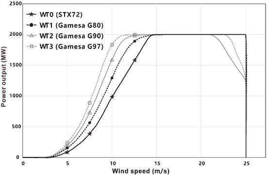
Figure 4.
Power curves of 2 MW wind turbines.
2.4. Cost of Tower and Rotor
The investment and operation costs according to HH are presented in Table 3. The costs were evaluated based on the 1 MW wind turbine and used in the TIC calculation of COE. The cost increase due to RD increase is presented in Table 4. The blade cost is determined considering the materials used, labor, profit and overhead, tooling, and transportation and is sensitive to the labor cost (LC) and material cost (MC) [21]. Other factors (overhead, tooling, and transportation) are fixed proportions accounting for 28% of the total rotor-related cost. Thus, only the costs of material (Equation (8)) and labor (Equation (9)), which were variable proportions, were considered, and 72% of the variable proportion except the fixed proportion out of the total cost was calculated using Equation (7).
Table 3.
Incremental cost of the 1 MW wind turbine. Source: Rehman et al. [8].
Table 4.
Costs of material and labor and total blade cost with rotor diameter. Source: Fingersh et al. [21].
3. Results
3.1. Regional Characteristics of OHH
OHH was calculated throughout all regions in South Korea, and its distribution is shown in Figure 5. Figure 5 shows a clear difference in OHH distribution according to the geographical conditions; the calculated OHH in the inland plain was 75 m~82 m, whereas that in the mountain or onshore sites was 60 m~70 m.
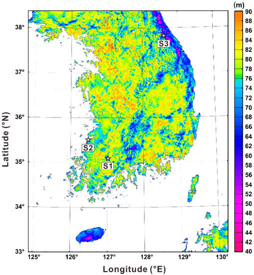
Figure 5.
Distribution of optimal hub height for WT0.
Figure 6 shows the COE curves at three typical sites (inland, onshore, and mountain) where the wind farms are currently operating, with the OHH, minimum COE, and wind profile exponent at each site presented in Table 5. For the inland site (S1), the highest OHH among the three sites was 74 m, followed by the onshore site (S2) with 63 m and the mountain site (S3) with 61 m. The calculated OHH in most sites was lower than the GHH of the MW-capacity wind turbine. In particular, OHHs in onshore and mountain sites were approximately 10 m lower than that of inland. If the onshore TIC is applied to that of offshore for approximation, for which calculating the construction cost is difficult due to the lack of cost information, OHH offshore is calculated to be 40 m or lower, which is fairly lower than that of onshore. Note, however, that this OHH is neither valid nor realistic considering the rotor length.
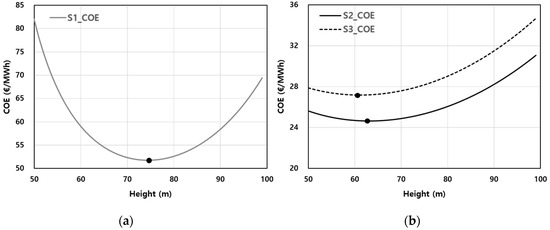
Figure 6.
COE curves by hub height and OHH (points) at the three sites. (a) S1; (b) S2 and S3.
Table 5.
Comparison of the calculated results at the three sites. OHH, optimal hub height; GHH, general hub height.
The reason for the difference in OHH by site can be found in the wind profile of each site (Figure 7). Specifically, the wind profile at (S1) (inland site) showed that the mean wind speed was lower than 4 m s−1, which is almost the cut-in speed of wind turbine WT0 at an approximate height of up to 50 m, followed by low AEP at 50 m or lower. Since the mean wind speed was higher than the cut-in speed at a height above 50 m, AEP increased, with the minimum COE found at a relatively high HH compared to that of other sites. In the inland site, the lower layer in the wind profile had a low wind speed due to the surface friction, which did not produce sufficient AEP. This was why OHH had to be high. In contrast, the mean wind speeds in the onshore (S2) and mountain (S3) sites exceeded the cut-in speed at a height below 50 m. Since S2 had the highest mean wind speed among the three sites, the minimum COE was also the lowest at 24.7 € MWh−1.
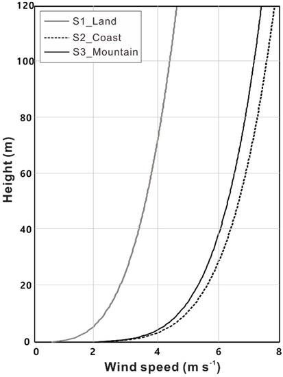
Figure 7.
Mean wind speed profile at the three sites (S1, S2, and S3).
3.2. Calculation of RD to Compensate for AEP
The calculated OHHs in most regions in South Korea were less than GHH. If wind turbines are installed according to the calculated OHH, it can reduce the cost required to construct a tower, which then leads to the minimization of COE; thus resulting in improvements in terms of economic feasibility. Note, however, that the reduction in HH will result in loss of AEP according to the reduction of wind speed in a rotor area. A power production loss of 5% is expected to occur if the OHH of the S1 site is changed to 74 m instead of using GHH. In the same manner, S2 and S3 will experience loss of AEP by 13% and 12%, respectively. In other words, lower HH means larger loss of AEP. This correlation is also applied to onshore and mountain sites where the mean wind speed is relatively stronger than that of inland.
This can be a drawback of the OHH calculation algorithm, which minimizes COE. If the goal is to maximize AEP, it is necessary to have a method of compensating for the loss of AEP due to OHH. This study derived a linear regression equation between RD and AEP after calculating the AEP of three types of wind turbines (WT1, WT2, WT3), which had longer RD than that of WT0 as the reference wind turbine to compensate for the lost AEP due to OHH (Figure 8). Figure 8 confirms that an increase in RD by 1 m at HH of 60 m~100 m improves AEP by 54 MWh to 64 MWh, and this trend is common in all regions in South Korea.
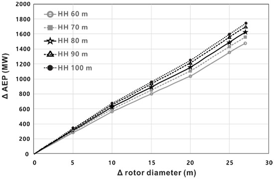
Figure 8.
Increment of annual energy production (AEP) with increment of rotor diameter at different hub heights.
Figure 9 shows the mapping of RD increment in South Korea to compensate for AEP loss due to OHH. Compared to Figure 5, Figure 9 indicates that a large RD increment is needed because of the large AEP loss in onshore and mountain sites where OHH was calculated to be lower than GHH. The RD increments at the three sites for AEP loss compensation, as analyzed above, were 2.1 m, 5.8 m, and 6.6 m, respectively (Table 6).
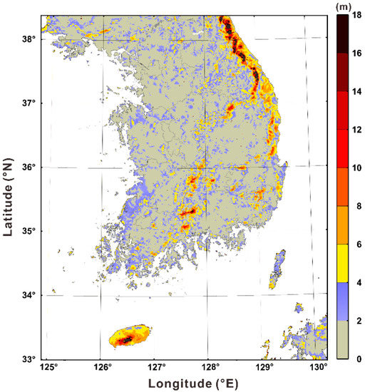
Figure 9.
Distribution of increment rotor diameter for compensating for AEP loss.
Table 6.
AEP loss due to decreased hub heights and gain owing to increased rotor diameter at the three sites. RD, rotor diameter.
3.3. Discussions
The OHHs in South Korea were distributed within 50 m~90 m, and a regional difference existed according to the geographical characteristics. OHH was also calculated to be a value below GHH in most regions. When HH was lower than GHH, both AEP and TIC were reduced, but COE was reduced because the reduction in TIC was larger (Figure 10a). This was why the minimum COE was derived at a height below GHH. This characteristic was more noticeable in S2 and S3 where the wind speed was higher, by which lower OHHs were calculated in S2 and S3. In contrast, the differences in the reduction rates of AEP and TIC decreased with higher OHH, and there was no significant difference near GHH. This was the reason for the small change in COE at the S1 site, where OHH was calculated to be 74 m. The increase rate of AEP at sites whose OHH was higher than GHH was higher than the increase rate of TIC. This was why a lower COE was calculated at high OHH than that of GHH. Most of these sites were low-wind speed (less than 5 m s−1 mean wind speed) sites that did not produce sufficient AEPs at a lower height below HH. Thus, OHH was calculated to be 80 m, wherein an increase in AEP was larger than that of TIC.
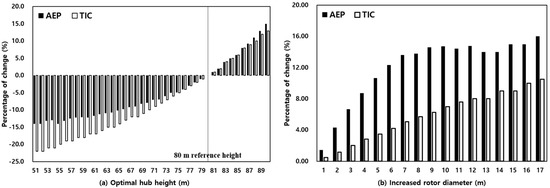
Figure 10.
Percentage change for AEP and total investment cost (TIC) with respect to (a) OHH and (b) increment of RD.
In this study, RD was increased to compensate for AEP loss due to the reduction in HH, which reduced COE further. This was because the increase in AEP due to the increase in RD was larger than the increase in cost owing to the increase in RD, as shown in Figure 10b. The sites that needed AEP loss compensation through the increase in RD were relatively high-wind speed sites, which was why the power of the wind turbine proportional to the cubic area of wind speed was also large. The reduced COE as a result of the AEP loss compensation was 13% compared to that of GHH, which was larger than the reduction rate of OHH (7%) (Table 7).
Table 7.
COE by 80 m, optimal hub height, and optimal hub height + rotor diameter.
The reduction in COE through the increase in RD was also consistent with the trend of the large size of wind turbines [22]. Note, however, that the calculated OHHs in this study showed a different trend. COE was minimized with lower OHH than GHH in high-wind speed sites but with higher OHH in low-wind speed sites. In other words, the characteristic of OHH differed according to the characteristics of the regional wind profile. Note that this study did not consider the limitation of the wind turbine class according to strong winds and turbulence intensity.
4. Conclusions
This study calculated AEP according to the changes in HH, using the time-series wind speed profile data of the wind resource map in South Korea and proposed an algorithm to find the OHH that minimized COE. In this study, not only was the AEP loss due to the lower OHH than GHH compensated for by increasing RD, a measure to reduce COE was presented as well.
The main study results are summarized as follows:
- (1)
- The inland plain site in South Korea exhibited minimum COE at a height of 74 m, which was similar to GHH. Note, however, that regions with relatively high wind speed, such as onshore or mountain sites, had OHHs of 63 m and 61 m or 17 m and 19 m lower, respectively, than that of the inland site. The economic feasibility of wind farms is expected to improve by minimizing COE in the future if OHH is selected according to the wind profile characteristics.
- (2)
- Unlike the study results of Lee et al. [5], the OHH calculation algorithm in this study presented a lower OHH than GHH in most sites except inland plain sites. OHH is determined according to the regional wind profile characteristics and is characterized to be higher than GHH if the wind resource is not sufficient in the lower layer of HH.
- (3)
- This study also verified the reduction in COE when RD increased to compensate for the AEP loss due to OHH. COE was reduced if RD increased in the entire area of South Korea. This was because the increase in AEP was larger than the increase in TIC, owing to the increase in RD.
- (4)
- This study was limited to onshore wind turbines. This was because the TIC of offshore wind turbines varied much more than that of onshore wind turbines, and the relevant database was not yet available. If the TIC database for offshore wind turbines is developed in the future, the OHH that can minimize COE even offshore will be calculated. Based on the results in this study, the offshore OHH is expected to be much lower than GHH.
Author Contributions
J.-T.L. designed and performed the simulations; H.-G.K. conceived a novel idea for the research theme and supervised the investigation; J.-Y.K. and Y.-H.K. supported the wind resource data; and J.-T.L. wrote the paper.
Funding
This research was conducted under the framework of the research and development program of Korea Institute of Energy Research (B9-2414).
Conflicts of Interest
The authors declare no conflict of interest.
Abbreviations
The following abbreviations are used in this manuscript:
| AEP | annual energy production |
| ASOS | automated surface observing system |
| AWS | automatic weather station |
| CAPEX | capital expenditure |
| COE | cost of energy |
| GHH | general hub height |
| HH | hub height |
| KMA | Korea Meteorological Administration |
| LC | labor cost |
| MC | material cost |
| OHH | optimal hub height |
| OPEX | operation expenditure |
| RD | rotor diameter |
| RDAPS | regional data assimilation and prediction system |
| REWS | rotor equivalent wind speed |
| RPM | revolutions per minute |
| SBL | surface boundary layer |
| TIC | total investment cost |
| WRF | weather research and forecasting |
| WT | wind turbine |
References
- Turbines, W. Part 1: Design Requirements, IEC 61400-1; International Electrotechnical Commission: Geneva, Switzerland, 2005. [Google Scholar]
- Letcher, T.M. Wind Energy Engineering: A Handbook for Onshore and Offshore Wind Turbines; Academic Press: Cambridge, MA, USA, 2017. [Google Scholar]
- Marmidis, G.; Lazarou, S.; Pyrgioti, E. Optimal placement of wind turbines in a wind park using Monte Carlo simulation. Renew. Energy 2008, 33, 1455–1460. [Google Scholar] [CrossRef]
- Emami, A.; Noghreh, P. New approach on optimization in placement of wind turbines within wind farm by genetic algorithms. Renew. Energy 2010, 35, 1559–1564. [Google Scholar] [CrossRef]
- Meyers, J.; Meneveau, C. Optimal turbine spacing in fully developed wind farm boundary layers. Wind Energy 2012, 15, 305–317. [Google Scholar] [CrossRef]
- Stevens, R.J. Dependence of optimal wind turbine spacing on wind farm length. Wind Energy 2016, 19, 651–663. [Google Scholar] [CrossRef]
- Lee, J.; Kim, D.R.; Lee, K.-S. Optimum hub height of a wind turbine for maximizing annual net profit. Energy Convers. Manag. 2015, 100, 90–96. [Google Scholar] [CrossRef]
- Rehman, S.; Al-Hadhrami, L.M.; Alam, M.M.; Meyer, J.P. Empirical correlation between hub height and local wind shear exponent for different sizes of wind turbines. Sustain. Energy Technol. Assess. 2013, 4, 45–51. [Google Scholar] [CrossRef]
- Maki, K.; Sbragio, R.; Vlahopoulos, N. System design of a wind turbine using a multi-level optimization approach. Renew. Energy 2012, 43, 101–110. [Google Scholar] [CrossRef]
- Mirghaed, M.R.; Roshandel, R. Site specific optimization of wind turbines energy cost: Iterative approach. Energy Convers. Manag. 2013, 73, 167–175. [Google Scholar] [CrossRef]
- Stanley, A.P.; Ning, A.; Dykes, K. Optimization of turbine design in wind farms with multiple hub heights, using exact analytic gradients and structural constraints. Wind Energy 2019, 22, 605–619. [Google Scholar] [CrossRef]
- Clack, C.T.; Alexander, A.; Choukulkar, A.; MacDonald, A.E. Demonstrating the effect of vertical and directional shear for resource mapping of wind power. Wind Energy 2016, 19, 1687–1697. [Google Scholar] [CrossRef]
- Janjić, Z.I. The step-mountain eta coordinate model: Further developments of the convection, viscous sublayer, and turbulence closure schemes. Mon. Weather Rev. 1994, 122, 927–945. [Google Scholar] [CrossRef]
- Hong, S.-Y.; Dudhia, J.; Chen, S.H. A revised approach to ice microphysical processes for the bulk parameterization of clouds and precipitation. Mon. Weather Rev. 2004, 132, 103–120. [Google Scholar] [CrossRef]
- Niu, G.Y.; Yang, Z.L.; Mitchell, K.E.; Chen, F.; Ek, M.B.; Barlage, M.; Kumar, A.; Manning, K.; Niyogi, D.; Rosero, E.; et al. The community Noah land surface model with multiparameterization options (Noah-MP): 1. Model description and evaluation with local-scale measurements. J. Geophys. Res. Atmos. 2011, 116. [Google Scholar] [CrossRef]
- Kim, H.-G.; Kang, Y.-H. The 2010 wind resource map of the Korean Peninsular. J. Wind Eng. Inst. Korea 2012, 16, 167–172. [Google Scholar]
- Kim, H.-G.; Kang, Y.-H.; Yun, C.-Y. Comparative Analysis on Commercial Wind Resource Maps of South Korea. J. Wind Eng. Ins. Korea 2015, 19, 9–14. [Google Scholar]
- Scheurich, F.; Enevoldsen, P.B.; Paulsen, H.N.; Dickow, K.K.; Fiedel, M.; Loeven, A.; Antoniou, I. Improving the accuracy of wind turbine power curve validation by the rotor equivalent wind speed concept. J. Phys. Conf. Ser. Ger. 2016, 753, 072029. [Google Scholar] [CrossRef]
- Wagner, R.; Cañadillas, B.; Clifton, A.; Feeney, S.; Nygaard, N.; Poodt, M.; St Martin, C.; Tüxen, E.; Wagenaar, J.W. Rotor equivalent wind speed for power curve measurement–comparative exercise for IEA Wind Annex 32. J. Phys. Conf. Ser. Den. 2014, 524, 012108. [Google Scholar] [CrossRef]
- Wagner, R.; Antoniou, I.; Pedersen, S.M.; Courtney, M.S.; Jørgensen, H.E. The influence of the wind speed profile on wind turbine performance measurements. Wind Energy 2019, 12, 348–362. [Google Scholar] [CrossRef]
- Fingersh, L.; Hand, M.; Laxson, A. Wind Turbine Design Cost and Scaling Model; No. NREL/TP-500-40566; National Renewable Energy Lab. (NREL): Golden, CO, USA, 2006.
- Wiser, R.; Hand, M.; Seel, J.; Paulos, B. Reducing Wind Energy Costs through Increased Turbine Size: Is the Sky the Limit? Lawrence Berkeley Natl. Lab. 2016. [Google Scholar]


© 2019 by the authors. Licensee MDPI, Basel, Switzerland. This article is an open access article distributed under the terms and conditions of the Creative Commons Attribution (CC BY) license (http://creativecommons.org/licenses/by/4.0/).