1. Introduction
Through long-time operation experience accumulation and continuous research, the parabolic trough solar thermal power plant (PTSTPP) is considered as the ripest in technique and most commercialized concentrating solar power technology [
1]. The parabolic trough solar field (PTSF), where solar energy is collected and converted to the thermal energy, is the component most worth exploring in a PTSTPP [
2]. In a representative PTSF, the heat transfer fluid (HTF) is distributed by the cold header and harvested by the hot header. Several parallel loops connect the cold and hot headers; each loop consists of a series of parabolic trough collectors (PTC), and the cold HTF is heated to a high temperature as it flows through the PTC loop. Finally, the hot HTF is pumped into the power block to produce the steam. As the solar irradiance and thermal requirement change, three parameters are used to adjust the flow rate of the HTF to meet the outlet temperature demand: the opening of the control valve in headers, the opening of the control valve in PTC loops, and the pump frequency [
3].
The majority of the published studies that research the PTSF place emphasis on a thermal perspective. Forristall et al. [
4] developed a detailed thermal steady-state model of the PTC, which is validated by the test results of a SEGS LS-2 solar collector [
5]. Stuetzle et al. [
6] built a thermal dynamic model of the PTC to study the control algorithm of a plant, and their measured data validated this model. Camacho et al. [
7] developed a simplified thermal dynamic model of the PTC, in which both the heat loss and heat convective coefficient are fitted as polynomials in the temperature. Padilla et al. [
8] and Hachicha et al. [
9] improved the thermal model in two ways: implementing a more comprehensive radiative analysis and considering that the solar flux distribution around the receiver is nonuniform, respectively. Yılmaz et al. [
10] developed a comprehensive thermo-mathematical model, whose detailed optical and thermal analysis in this model allow the model to simulate more accurate results for the optical loss, heat loss, and thermal efficiency. Behar et al. [
11] improved on the accuracy of thermal performance prediction of the PTC in another way, i.e., developing a novel model that can consider the flow rate variation by adapting an optimization procedure of the HTF outlet temperature.
In effect, in a large-scaled PTSF, because the flow rate in the individual PTC loop is unknown and determined by the layout, pump head, and flow resistance, a detailed thermal model of the PTC is insufficient to understand the performance of the PTSF comprehensively. Therefore, in some studies, the PTSF is regarded as a complex piping network, whose thermal hydraulic characteristics are researched. The symmetrical and uniform flow distribution of the PTSF was assumed to simulate the PTSTPP in the System Advisor Model (SAM), which was developed by the National Renewable Energy Laboratory (NREL) and Sandia National Laboratory [
12]. Abutayeh et al. [
13] spelled out the presence of unbalanced flow distribution in the PTSF and proposed a method to amend it. Giostri [
3] studied the behavior of the PTSF under a variety of thermal transients based on a thermal hydraulic model, which contained a thermal dynamic part and a hydraulic steady pipe network part. A virtual solar field (VSF), which was developed by the German Aerospace Centre (DLR) [
14], applied a thermal hydraulic model similar to [
3] to simulate the behavior of the whole PTSF, and the operating data from Andasol-3 validated the model. Ma et al. [
15] revealed the relationship between the flow distribution and flow resistance of the PTSF, and then verified the method proposed in [
13] based on a thermal hydraulic dynamic model (THDM) and tested data obtained from a pilot plant.
Two aspects need to be improved in the existing thermal hydraulic models of the PTSF, i.e., the lack of pump module and the unaccounted hydraulic transients. The former leads to the dependence on the inlet header flow rate in simulation and validation, and the latter obscures the PTSF specific behavior under the thermal and hydraulic transients. There are two reasons for the difficulty of solving these problems by directly employing the transient hydraulic model in the water distribution system (WDS), of which the numerical method is relatively ripe [
16,
17,
18]. One is that in the WDS, the water is often assumed to be incompressible, while in the PTSF, the expansion and contraction of the HTF are non-negligible due to the significant temperature difference. The other is that the flow resistance is considered as a constant or merely a function of the flow velocity in the WDS, while it is a more complex function under the influence of temperature variation in the PTSF.
Besides, developing an effective control strategy of the PTSF is also dependent on the integrality of the thermal hydraulic model. Ref. [
19] pointed out that the header control valves (HCVs) are used to control the flow rate and outlet temperature of the subfield in a real operated PTSTPP. [
13] indicated that the automatic balancing valves can be used for PTSF control when the spatial variation of solar irradiance is an issue. Refs. [
14] and [
20] indicated that the loop control valves (LCVs) have the potential to improve the PTSF performance. However, the lack of a refined model increases the difficulty of calculating the valves opening and simulating the PTSF characteristics under varied solar irradiance.
To overcome the above problems, as well as improve the operational performance and controllability of the PTSTPP, a comprehensive thermal hydraulic model (CTHM) of the PTSF based on a pilot plant in Beijing is presented in this paper. The CTHM is improved based on the THDM developed in [
15]. The optical and thermal analysis of the PTC, the flow characteristics of pipe, pipe fitting, pump, and the valves are all considered in the CTHM. A novel numerical method, which is based on graph theory and the Newton–Raphson method, is developed to solve the CTHM. Moreover, a cold test and a hot test are implemented to validate the CTHM under thermal and hydraulic disturbance.
Compared with the THDM and other existing models, the CTHM has three main advantages. Firstly, adding the pump module establishes the relationship among the pump capacity, flow resistance, and the temperature. This improvement further makes the required input parameters get rid of the dependence on the total flow rate. Secondly, the CTHM contains both the hydraulic and thermal inertia, and this leads to more accurate results in the transient simulation. Finally, a more comprehensive model can widen and deepen the research on the PTSF; the CTHM can be applied to simulate the behavior of the PTSF under various disturbances and study the control strategy of the PTSF under uniform or nonuniform solar irradiance.
2. Description of the PTSF of a 1 MW Pilot Plant
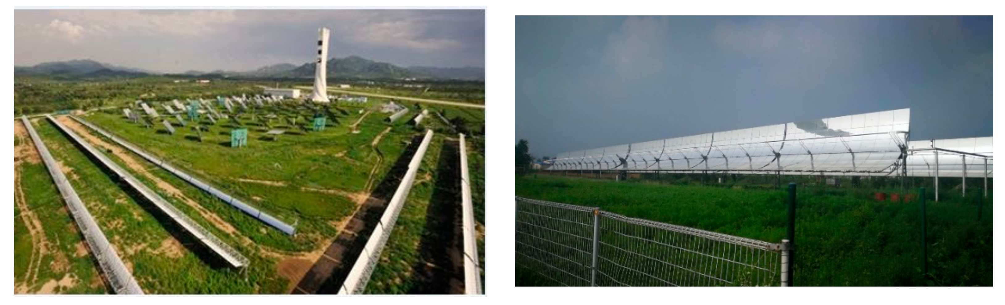
The Badaling parabolic trough solar power pilot plant, which is the first operational PTC solar thermal plant on the MW scale in China, is situated in Yanqing at a latitude of 40.5°N and a longitude of 115.94°E. A view of the pilot plant is shown in
Figure 1.
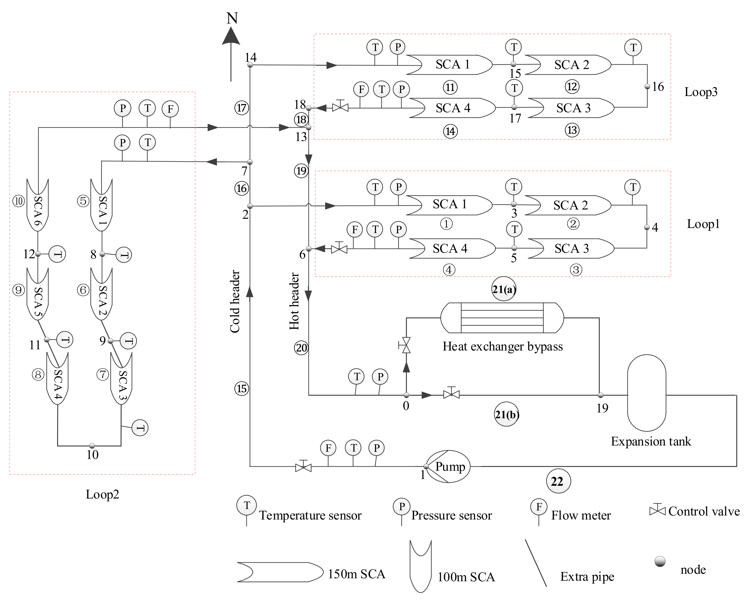
As illustrated in
Figure 2, two east–west layout loops (Loop 1 and Loop 3) with 4150 m long solar collector assemblies (SCAs) and one south–north layout loop (Loop 2) with 6100 m long SCAs together form the principal part of the PTSF. Besides, an extra pipe is placed in Loop 2 for a study of flow balance [
15]. An HCV and three LCVs are used to manipulate the total flow rate and flow distribution. A kind of synthetic oil named Therminol VP-1, of which the physical properties can be fitted into some polynomials in temperature based on the tested data [
13], is used as the HTF in the pilot plant, while the more detailed information about the physical properties of the HTF is summarized in
Appendix A.
The present study involves two kinds of pipes in the PTSF, i.e., the absorbed pipe covered with an evacuated glass envelope, and the insulated pipe (header). Hereafter, the symbols, which are concerned with the pipe, will represent the former with the subscript abs, and represent the latter with the subscript ins. Moreover, the symbols without any subscripts mean that they are universal for both types. Specific characteristics of the PTC, header, pump, and valve are described in more detail below.
2.1. The PTC and Header
In the relevant published studies [
1,
2,
3,
4,
5,
6,
7,
8,
9,
10,
11,
12], the thermal model of the PTC developed in [
7] is applied in this paper. The effectiveness of this model has been validated by the tested data regardless of the simplified thermal loss of the PTC [
7,
15].
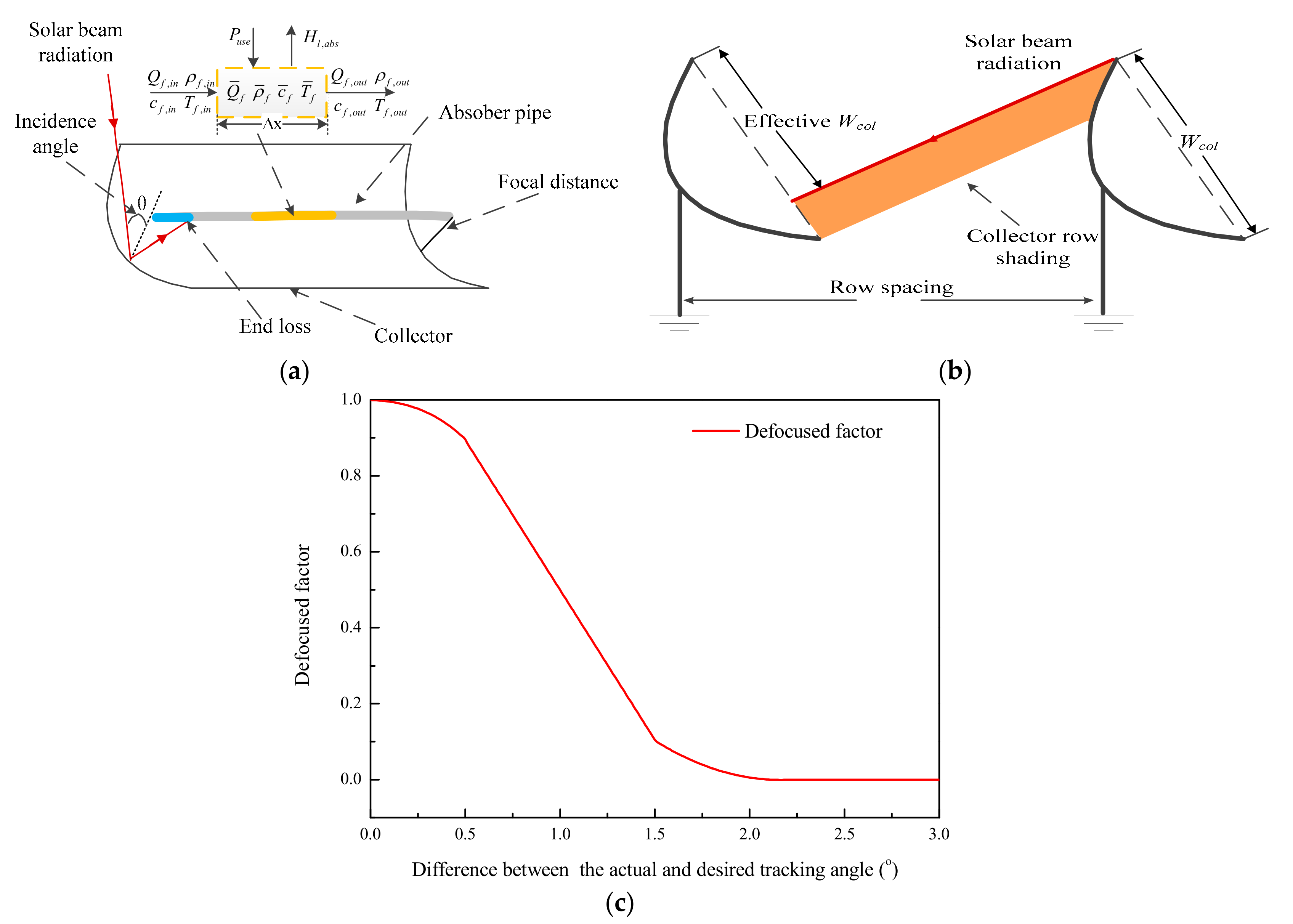
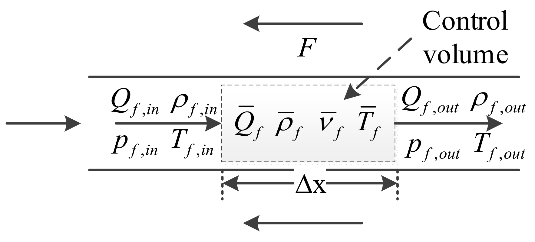
As shown in
Figure 3a, the energy equation of the control volume with an axial length of △
x can be given by [
7]:
where the subscript f represents the HTF,
Q,
ρ,
T, and
c represent the volume flow rate, density, temperature, and specific heat capacity, and
D and
A are the diameter and sectional area.
Hl,abs represents the heat loss of the absorber per meter, which is caused by the temperature difference between the absorber tube and the exterior glass envelope, and can be simplified as a polynomial in
Tabs.
Puse in Equation (1) is the solar thermal power supplied to the absorbed pipe per meter, which is given by [
21]:
where
Wcol represents the collector width,
I represents the direct normal irradiance (DNI), and
κ is the incidence angle (
θ) modifier, which is used to account for all geometric and optical losses because of an incident angle of more than 0°.
ηo is the optical efficiency of the PTC, which is the product of the clean mirror reflectivity (
rcl), the transmittance of the glass envelope (
τ), the absorbance of the absorber pipe (α), and the intercept factor (γ). β is the defocused factor, which is used for considering the loss of efficiency caused by the difference between the actual and desired tracking angle. As shown in
Figure 3c, the trend of β can be simulated by the Solartrace tool [
3].
fend and
fshd are two factors due to end loss and row shadowing; the schematic diagram of
fend and
fshd is shown in
Figure 3a,b respectively. Expressions of these two factors can be given by [
3]:
where
ω represents the zenith angle, and
lSCA,
lrs, and
lfd are the length of the SCA, row spacing, and focal distance, respectively.
h in equations (1) and (2) is the convection heat transfer coefficient between the absorber inner surface and the HTF, which can be given by [
4]:
where
Re,
Nu, and
Pr are the Reynolds number, Nusselt number, and Prandtl number, respectively.
k is the thermal conductivity. In the normal operation of the pilot plant, the variation range of the Re and
Pr are about 1 × 10
4 <
Re < 9 × 10
5 and 4.5 <
Pr < 45; these two parameters are within the range of application of Equation (8), which is valid for 2300 <
Re < 5 × 10
6 and 0.5 <
Pr < 2000 [
4].
More than the HCE absorber pipes, thermal losses exist in the insulated pipes (headers). In this work, the mineral wool is used as the thermal insulation material, and the thermal losses of the insulated pipes can be calculated under an assumption of neglecting the thermal resistances of the exterior air film and pipe walls [
21], which is given by:
where
is the thermal conductivity of the pipe insulation at the average temperature of
and
Tins, and
Ta and
δ are the insulation thickness and ambient temperature, respectively. The value of
can be fitted into a polynomial at the average temperature [
21].
The thermal and optical parameters, the geometry of the absorber and the header are listed in
Table 1, where formulas of the incidence angle modifer is given by [
21], and formulas of the heat loss r is supplied by the manufacturer. Other header parameters that are not included in the table, such as the length from pump to Loop 1, the length from Loop 3 to expansion, the expression of
, and so on, can be measured from the design drawing.
Equations (1)–(9) together form the thermal part of the CTHM, this part is applied to simulate the outlet temperature and update the properties of the HTF.
2.2. Pump and Valve
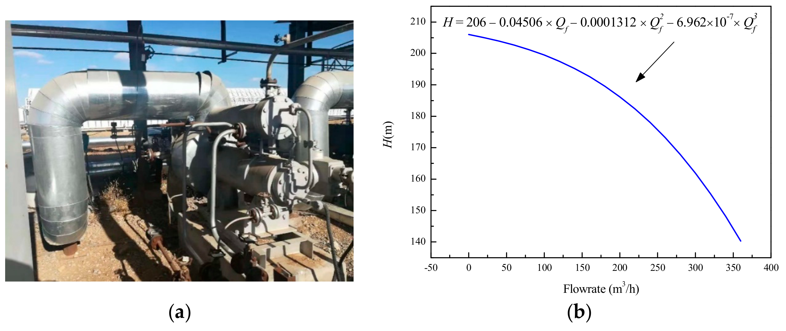
As shown in
Figure 4a, a canned centrifugal pump is chosen to circulate the HTF in the pilot plant, the capacity, head, and efficiency at design condition are 99 m
3/h, 200 m, and 45%, respectively. In normal hydraulic calculations, the pump head is usually fitted into a polynomial in the capacity according to the pump’s performance curve, and this method has been applied to the PTSF by defining the polynomial with a series of universal coefficients [
22,
23]. In this study, as shown in
Figure 4b, the polynomial of the pump head can be given in a more specific way based on the pump’s performance curve supplied by the manufacturer.
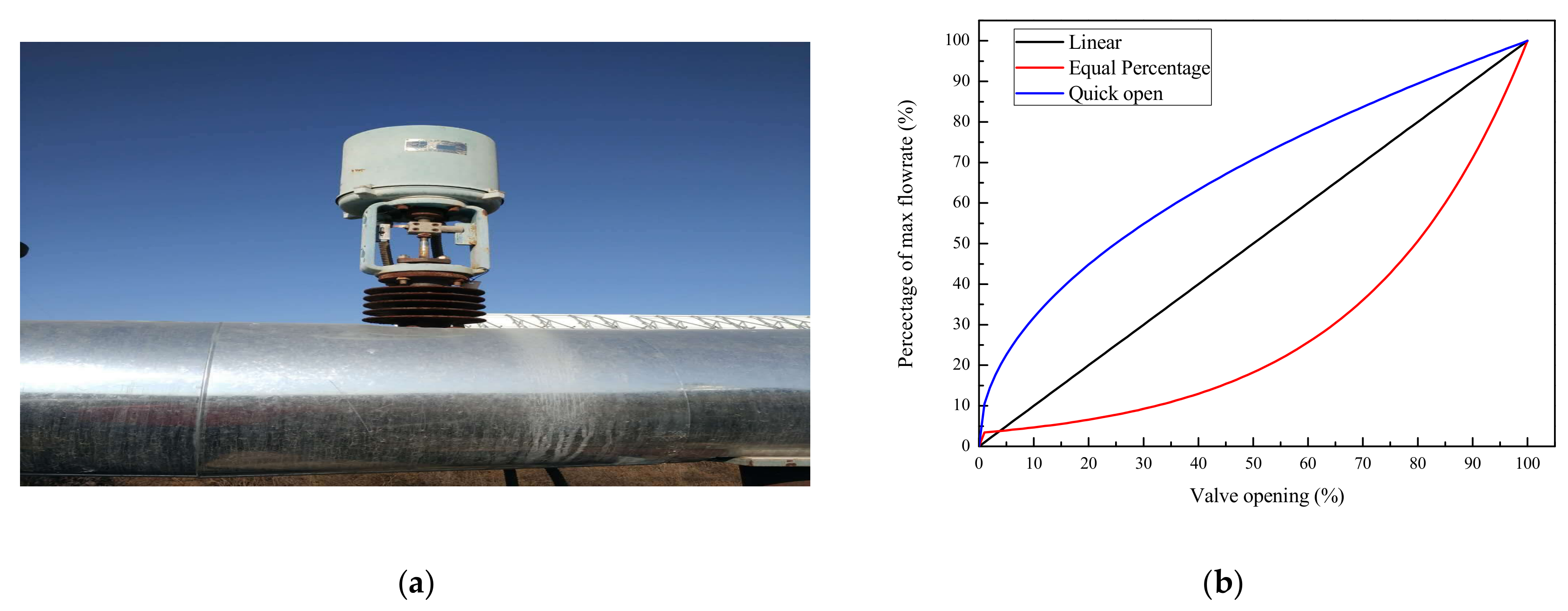
A typical control valve in the PTSF is shown in
Figure 5a, the electric actuator manipulates the opening of the valve. In general, as shown in
Figure 5b, the control valve has three inherent flow characteristics [
24], i.e., linear, quick open, and equal percentage. In the pilot plant, both the LCVs and HCVs are chosen to have the flow characteristics with equal percentage.
2.3. Measurement and Uncertainty
In the PTSF of the pilot plant, the DNI, flow rate, temperature, and pressure of the HTF in the header and three loops, the opening of the valve, the actual tracking angle, and the ambient temperature are the main parameters that need to be measured; the information of measurements and their uncertainty are summarized in
Table 2.
5. Model Applications
After the accuracy and availability of the CTHM are validated, two potential abilities of the model are presented in this section. First, the relationship between the thermal and hydraulic transients are revealed by two simulating cases. Secondly, two simple feedforward control strategies are introduced and verified through the CTHM. In all of the simulations, the ambient temperature and inlet temperature of the header remain 25 °C and 290 °C, respectively.
5.1. Transients Simulating
As a complex piping network, the thermal effect is the biggest difference between the WDS and the PTSF. Two cases are conducted to simulate how the thermal transients influence the hydraulic state. Ma et.al [
15] pointed out that the PTSF of the pilot plant can achieve balanced flow distribution when the openings of the three LCVs are 58%, 100%, and 60%, respectively; these values will be maintained in these two cases.
Case 1, which lasts for 1.3 h, is implemented for simulating the impacts of DNI saltation on the total flow rate and pump pressurizing of the PTSF. As shown in
Figure 16a, the DNI changes from 0 to 800 W/m
2 at 0.4 h and turns back into 0 at 0.9 h, and these two disturbances cause a drastic fluctuation in the header flow rate, as shown in
Figure 16b. At 0.4 h, as shown in
Figure 16b, the inlet and outlet header flow rate present two different trends. The peaking of heat gain causes an expansion of the HTF and further leads to the increasing velocity; this will result in an increase of the pump pressurizing (as shown in
Figure 16c) and a reduction of pump capacity (inlet header flow rate). Meanwhile, the viscosity of the HTF decreases with the temperature rise (as shown in
Figure 16d). Together with the density and viscosity, the total flow resistance and pump pressurizing will reach a local maximum and begin to decrease; when the effect of expansion surpasses the effect of viscosity reduction, the total pressure drop increases again, and the pump capacity decreases until it reaches a steady state. Similar reasons can demonstrate the fluctuation of the header inlet flow rate, and pump pressurizing happens when the DNI vanishes. For the header outlet flow rate, according to Equation (12), the dramatic expansion and contraction of the HTF caused by the DNI saltation will be embodied in the outlet flow rate, which causes an opposite trend between the inlet and outlet flow rate.
Case 2, which lasted for 1.7 h, was conducted for simulating how the thermal effect influences the flow distribution of the PTSF; in this case, the DNI is maintained at 800 W/m
2 throughout the whole process. As shown in
Figure 17a, the SCAs in Loop 1 will be defocused in a positive (from one to four) and a negative (from four to one) sequence. The reasons for the fluctuation of flow rate and pump pressurizing at the time of defocus are demonstrated in Case 1. As shown in
Figure 17b,c, both defocus sequences cause an increase of the header flow rate and a reduction of pump pressurizing. This is because the HTF will stop expanding and has a lower velocity in the defocused SCAs compared with a focused one; this further leads to a lower pump pressure and higher pump capacity. This effect is presented in a more obvious way in the comparison of flow rate among the three loops shown in
Figure 17b; the flow rate in the defocused Loop 1 increases step-by-step compared with the other two focused loops due to its lower pressure drop. Besides, compared with the negative defocused sequence, the cold HTF will flow over longer distances when the SCAs are defocused in a positive sequence. As a result, the higher flow rate and lower pump pressure exist in the positive defocused sequence due to the lower flow resistance. Finally, the HTF in the SCAs, which is closer to the inlet, has greater thermal inertia than the SCAs near the outlet; this causes the difference of outlet temperature between the two opposite sequences of defocus shown in
Figure 17d.
The density, specific heat capacity, and the viscosity are the most relevant properties to the thermal hydraulic characteristics of the PTSF. Based on the simulation results of the above two cases, it can be found that when the inlet temperature of the header stays the same, the effect of density is the most influential property, followed by the specific heat capacity and viscosity. From a thermal perspective, although the specific heat capacity increases with the temperature, the thermal inertia decreases with the temperature because of the reduction of density. From a hydraulic perspective, although the viscosity decreases with the temperature, the pressure loss increases with the temperature because the expansion of the HTF causes a greater velocity.
5.2. Feedforward Control Strategy
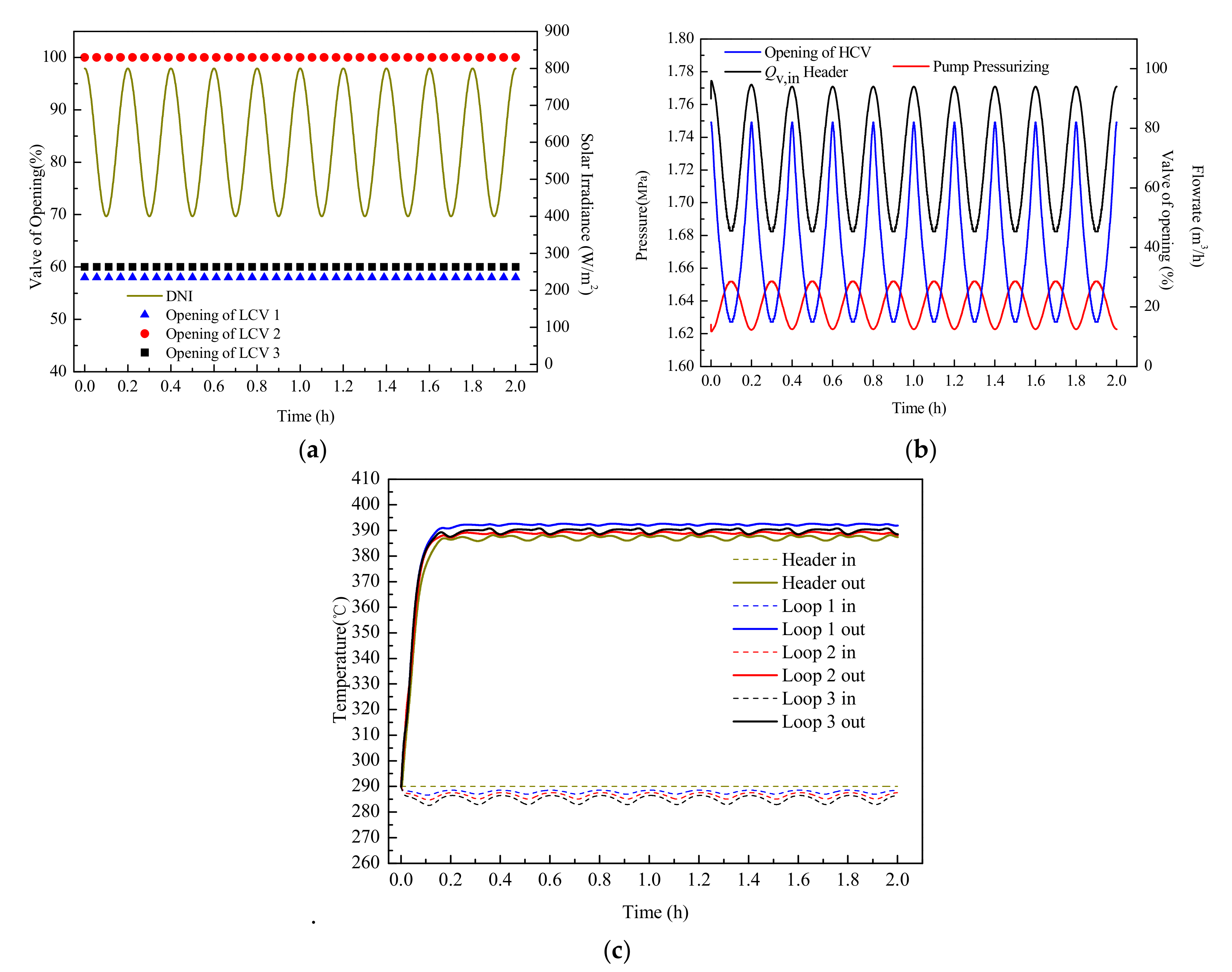
An important function of the CTHM is being used for study of control strategy; two feedforward control strategies based on the CTHM are introduced in this section. In both strategies, the header inlet temperature is set at 290 °C, and opening of the HCV and the LCVs are the control variables that control the outlet temperature of the header and three loops at 390 °C.
The first strategy is studied under a uniform solar irradiance; as shown in
Figure 18a, the DNI of the whole PTSF varies with a cosine disturbance from 800 W/m
2 to 400 W/m
2, of which the period is 0.2 h. Due to the uniformity of the DNI, a balanced flow distribution must be maintained for the same outlet temperature of the three loops, so the openings of the three LCVs are kept constant. The ideal flow rate under different DNI values can be calculated according to the thermal part of the CTHM, while the opening of the HCV and pump pressurizing can be solved according to the hydraulic part of the CTHM and the calculated ideal flow rate; these results are shown in
Figure 18b. The control results of the outlet temperature are shown in
Figure 18c, the outlet temperatures of the three loops and header are all very close to 390 °C, and the small-range fluctuations of the outlet temperature in the three loops and headers are caused by the heat loss in the header, which varies with the flow rate.
The second strategy is researched under a nonuniform solar irradiance. As shown in
Figure 19a, the DNI values in Loop 1 and Loop 3 are kept at 800 W/m
2, while for Loop 2, the DNI varied in a similar way as shown in
Figure 18a. The balance of flow distribution must be thrown off due to the nonuniformity of DNI, so the opening of three LCVs should be recalculated to meet the varied DNI. The ideal flowrate distribution can also be solved by the thermal part of the CTHM, while the openings of the HCV and LCVs can be calculated in two steps. First, we set the opening of the LCV in Loop 3 at 60% and calculated the opening of the LCVs in Loop 2 and Loop 3 with the method referenced in [
13] and [
15]. Second, we work out the opening of the HCV and pump pressurizing by the hydraulic part of the CTHM. The above results are shown in
Figure 19b: the opening of the LCVs in Loop 1 varied within a tiny scale, and the varied opening of the HCV and LCV in Loop 2 are the major variables for controlling the flow rate.
The good control results for the flow rate and outlet temperature are shown in
Figure 19c,d; the key presented in the results is that the fluctuation of the header flow rate can be centered on Loop 2 if the openings of the LCV and HCV vary in a similar way. These results verify the feasibility of PTSF control by the cooperation of LCVs and HCVs under a complex distribution of DNI and SCA performance in a large-scaled plant.
6. Conclusions
This paper mainly outlines a comprehensive thermal hydraulic model (CTHM) for the parabolic trough solar field (PTSF) based on a pilot plant. The CTHM is established and solved by a novel numerical method, validated by the experimental data based on the pilot plant, and applied to simulate the dynamic behavior and develop the control strategy of the PTSF under many types of disturbances. The main contribution of this paper is its development of a powerful model for the deeper study on PTSF. On the one hand, the total flow rate, flow distribution, pump head, and outlet temperature can be detailed and calculated by the CTHM under normal or disturbed conditions; on the other hand, when the value and distribution of the solar irradiance deviates from that of the design situation, the CTHM can also be used to calculate the opening of valves for the desired outlet temperature.
In this paper, all of work surrounds a 1 MW pilot plant, which is much smaller than a large-scaled commercial plant. However, all of the key factors (such as the unbalanced flow distribution) are included in the pilot plant, so the validity of the CTHM will always remain when it is applied to a large-scaled PTSF. In the future, the CTHM can play an important role in the further study of the commercial parabolic trough power plant, such as providing more detailed outlet parameters when combining the PTSF with a thermal storage system or power block, or using it to develop the optimal operation strategy.


