A Discussion on the Effective Ventilation Distance in Dead-End Tunnels

Abstract

Forcing ventilation is the most widely used system to remove noxious gases from a working face during tunnel construction. This system creates a region near the face (dead zone), in which ventilation takes place by natural diffusion, rather than being directly swept by the air current. Despite the extensive use of this system, there is still a lack of parametrical studies discerning the main parameters affecting its formation as well as a correlation indicating their interrelation. With this aim in mind, computational fluid dynamics (CFDs) models were used to define the dead zone based on the airflow field patterns. The formation of counter vortices, which although maintain the movement of air hinder its renewal, allowed us to discuss the old paradigm of defining the dead zone as a very low air velocity zone. Moreover, further simulations using a model of air mixed with NO₂ offered an idea of NO₂ concentrations over time and distance to the face, allowing us to derive at a more realistic equation for the effective distance. The results given here confirm the degree of conservativism of present-day regulations and may assist engineers to improve ventilation efficiency in tunnels by modifying the duct end-to-face distance.

1. Introduction

Underground ventilation provides enough airflow to the workings to dilute and remove noxious gases and dust. Furthermore, underground ventilation supplies O₂ where it has been depleted and controls temperature. Noxious gases may come from strata rock (e.g., CH₄, CO₂, H₂S, Rn), be generated by underground machinery (e.g., CO, CO₂, NO_x), or be a consequence of blasting operations (CO, NO_x) [1,2]. Two systems are used for mine ventilation purposes, namely, principal and ancillary. The former provides air to the overall mine, establishing general air circulation. The latter is used in developing workings and galleries and provides fresh air to specific areas in the mine. The ancillary ventilation of mine galleries is similar to that used in tunnels under construction. The main difference between them is that, for tunnel ventilation purposes, outside air is directly conducted to the face, whereas in mine ventilation fresh air has to be diverted from the main ventilation system into the working faces.

The favorite ventilation system for ancillary mine ventilation is the forcing system. Forcing is preferred over exhaust ventilation, as the fresh air coming along the roadway usually enters the duct straight away without sweeping the face first [3] (p. 7). The physics of this ventilating system is similar to a that of free jet that progressively opens, reducing its velocity until it reaches zero. The region in which the air is immobile is termed “the dead zone”, and it is separated by distance from the face “d_z” (Figure 1). In this zone, ventilation takes place by natural diffusion rather than being directly swept by the air current. The distance between the duct end and the dead zone is the air jet range, which is termed “the effective distance” (e_z). The sum of both distances is the space between the duct end and the face (d_s). The limit case occurs when there is no dead zone so that “e_z” is equal to “d_s”.

The most simple reference range for e_z is less than 15 m (e.g., [3] (p. 7)). Other authors consider “e_z” as a function of the gallery section (S) so that e_z be less than $4\sqrt{S}$ or less than $6\sqrt{S}$ (e.g., [4] (p. 381)). Moreover, others consider the gallery section and a parameter “a”, which is usually 0.07, in which case $e_z<0.5\sqrt{S \left(1+\frac{1}{2a}\right)}=4\sqrt{S}\simeq 12-15 \mathrm{m}$ [5] (p. 245). Finally, additional approaches consider the ventilation duct as a reference, in which case “e_z” should be 10–15 times as large as its diameter [6]. All legal requirements worldwide follow one of these recommendations, without getting into the physics of the dead zone formation.

Computational fluid dynamics (CFDs) has become an important tool for most fluid dynamics engineering problems, thus playing an emerging role in mine ventilation systems design [7]. Its popularity is mainly due to its low cost and capability of measuring parameters, which are difficult or almost impossible to obtain experimentally, as well as its fast assessment and adaptability to varying design conditions. In this context, CFDs may offer insight into the mechanics of dead zone formation.

The first CFDs in the field of mine ventilation were started by Herdeen and Sullivan (1993) and Srinivasa et al. (1993), who used a Eulerian–Lagrangian formulation. Since the apparition of modern commercial software, CFDs models have been used in several aspects of mine ventilation. Thus, extensive studies have been conducted in the field of dust transport (e.g., [7,8]) and heat transfer. The latter is important the case of heat fires and explosions in longwall working faces (e.g., [9,10]). Moreover, Sasmito et al. [11] studied air conditioning as a complement to ventilation for heat control in dead-end tunnels. Furthermore, Yuan and Smith [12] studied the low-temperature oxidation of coal using unsteady-state simulations. Likewise, Shi et al. [13] developed a CFDs model for coal spontaneous combustion under goaf gas drainage conditions.

As concerns auxiliary ventilation, Diego et al. [14] compared traditional and CFDs models for calculating losses in a dead-end circular tunnel, highlighting the advantages of CFDs over traditional calculations. Toraño et al. [15] studied auxiliary ventilation roadways driven with roadheaders, but their results cannot be directly transferred for dead-end tunnel ventilation. Sasmito et al. [16] performed a computational study on gas control in a room and pillar coal mine. Toraño et al. (2009) [17] modeled methane behavior, but did not consider blasting gases, in coal mines ancillary ventilation. Li, Aminossadati and Wu [18] studied ancillary ventilation in super large developments. Onder, Sarac and Cevik studied the ventilation of a cul-de-sac, but focused on fan–duct interaction rather than on the flow outside the duct. Fang, Yao and Lei conducted a parametrical study but did not consider the cross-sectional area as a variable [19]; thus, the magnitude of the effects associated with the whole set of parameters is yet to be established. Szlazak et al. [20] and Reed and Taylor [21] indicated that ancillary ventilation has been conducted under old-fashioned guidelines. As a consequence, it can be concluded that there is still a lack of knowledge concerning ventilation setup influence on dead zone formation in an empty heading. All things considered, the main aim of this study is to determine the correlations among the main factors influencing the effective distance in cul-de-sac ventilation so that their respective influences can be quantified. The following parameters are taken into account: tunnel section, flow rate and position with regard to the tunnel axis. This distance was first assessed based on the flow field patterns obtained, and later on a mixture model of air and NO₂.

The rest of the paper is organized as follows. Section 2 defines the geometries, exposes the discretization, presents the equations solved by the CFDs model, defines the boundary conditions, indicates the software configuration, describes the criteria followed for the delimitation of the dead zone and explains the mixture model. Section 3 discusses the delimitation of the dead zone and presents the correlation for dead-end-to-face distance, based on both flow field patterns and flow field patterns plus the mixture model correction. We conclude the paper in Section 4.

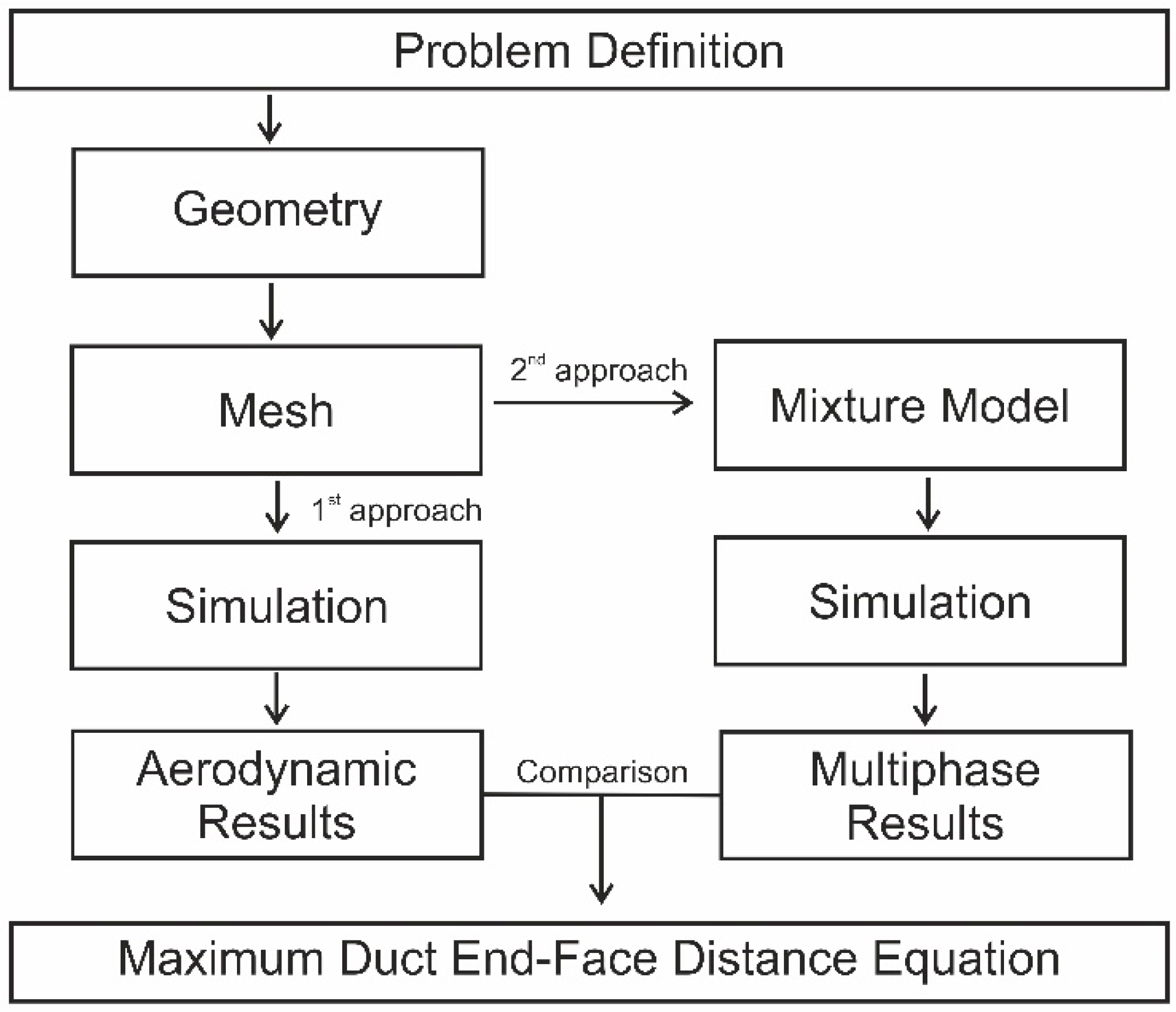
2. Materials and Methods

All the work was carried out by means of the ANSYS package, which allows for the modeling of different engineering problems using numerical methods. In this case, the hardware used to run the bulk of the simulations consisted in a cluster of computers equipped with i7-6800K processors and 32 GB DDR4 RAM. With these computers and the settings described later, each simulation was run for between 4 h and 5 h. Figure 2 illustrates a flow chart depicting the methodology followed by the authors.

2.1. Geometries

The geometry was generated using an ANSYS Design Modeler, commercial software, which is included in the ANSYS WorkBench package. A parametric study was performed for the study. The geometries of the tunnel and the variables considered are given in Figure 3. Face-to-duct end distances were large enough to ensure that the flow was not influenced by boundary conditions. The tunnel profile was defined for a regular tunnel section. All of the analyzed profiles were concentric to that depicted in Figure 3. Common sections for mine ducts were retrieved from commercial catalogs and particularly from [22] (p. 236). The parametrized geometry is specified in

Table 1. Geometrical parameters used for the parametric study.

Geometrical Parameters for Each Scenario		Parameter
		A	H	R	Rd	D	Ld	Lt	S
Units		m							m2
Scenario	1	5.4	1.8	2.7	1.8	0.54	50	100	21.17
	2	6	2	3	2	0.60			26.13
	3	7.2	2.4	3.6	2.4	0.72			37.63
	4	9	3	4.5	3	0.90			58.80

for the four scenarios considered.

2.2. Discretization

The geometry discretization was performed by means of ANSYS ICEM CFD. This software allows for the formation of high-quality hexahedral meshes based on the blocking method. Each of the meshes generated for the four scenarios had about one million cells (Figure 4a). The mesh quality was assessed by means of the angle criterion. This criterion takes into account the internal angles of each cell and seeks the maximum internal angle deviation from 90° for each element. Figure 4b shows that the mesh quality was above the typical quality criterion for CFDs purposes, which is 18°. In addition, most of the cell angles were close to the optimum value (90°).

In addition, a sensibility analysis of the mesh was also carried out. In Figure 5 the effective ventilation distance in front of the number of mesh cells in millions is shown. Three meshes were simulated (0.7 M/1 M/4 M cells) for scenario 2 and 20 m/s at the inlet boundary condition. It can be seen that the effective ventilation distance depends on the number of cells used, but the error committed with each of the meshes is negligible, as opposed to the value of the distance (about 1.5% for the mesh of 0.7 M cells). Nevertheless, in order to minimize the error while maintaining an optimum simulation time, the mesh of 1 million cells was selected for the subsequent experiments. The value for this mesh is near to the convergence value with a deviation of 0.3% (Figure 5), which is an assumable error.

2.3. CFDs Model

Since the Navier–Stokes equations cannot be solved analytically, the assessment of the flow pattern was performed by means of ANSYS Fluent software. This software solves the Navier–Stokes Equations (1)–(7) [23] using the finite volume model.

Continuity equation:

$$\frac{\partial \rho }{\partial t}+\nabla \ast \left(\rho \ast \overrightarrow{v_a}\right)=S_m.$$

(1)

Simplified to the problem:

$$\frac{\partial \left(\rho u\right)}{\partial x}+\frac{\partial \left(\rho v\right)}{\partial y}+\frac{\partial \left(\rho w\right)}{\partial z}=0.$$

(2)

Momentum conservation equation:

$$\frac{\partial }{\partial t}\left(\rho \overrightarrow{v_a}\right)+\nabla \ast \left(\rho \overrightarrow{v_a}\overrightarrow{v_a}\right)=-\nabla P+\nabla \ast \left(\stackrel{=}{\tau }\right)+\rho \overrightarrow{g}+\overrightarrow{F}.$$

(3)

Simplified to the problem and decomposed in three axes:

$$-\frac{\partial P}{\partial x}+\frac{\partial \left(\tau xx\right)}{\partial x}+\frac{\partial \left(\tau yx\right)}{\partial y}+\frac{\partial \left(\tau zx\right)}{\partial z}=\nabla \ast \left(\rho \overrightarrow{u}\overrightarrow{u}\right),$$

(4)

$$-\frac{\partial P}{\partial y}+\frac{\partial \left(\tau xy\right)}{\partial x}+\frac{\partial \left(\tau yy\right)}{\partial y}+\frac{\partial \left(\tau zy\right)}{\partial z}=\nabla \ast \left(\rho \overrightarrow{v}\overrightarrow{u}\right),$$

(5)

$$-\frac{\partial P}{\partial z}+\frac{\partial \left(\tau xz\right)}{\partial x}+\frac{\partial \left(\tau yz\right)}{\partial y}+\frac{\partial \left(\tau zz\right)}{\partial z}=\nabla \ast \left(\rho \overrightarrow{w}\overrightarrow{u}\right).$$

(6)

The stress vector was calculated as:

$$\tau =\mu \left[\left(\nabla \overrightarrow{v_a}+\nabla {\overrightarrow{v_a}}^T\right)-\frac{2}{3}\nabla \ast \overrightarrow{v_a}I\right].$$

(7)

2.4. Turbulence Model

The equations above were solved using the SIMPLE scheme for the pressure–velocity coupling. In addition, for turbulence modeling, a k-ε model was selected [24]. The k-ε model is a two-equation model, which aims at resolving the turbulence using two parameters: the turbulence kinetic energy (k) and the dissipation rate (ε).

The equations solved by this model are listed as Equations (8) and (9) [23]:

$$\frac{\partial }{\partial t}\left(\rho k\right)+\frac{\partial }{\partial x_i}\left(\rho k{u}_i\right)=\frac{\partial }{\partial x_j}\left[\left(\mu +\frac{{\mu }_t}{{\sigma }_k}\right)\frac{\partial k}{\partial x_j}\right]+G_k+G_b-\rho \epsilon -Y_M+S_k,$$

(8)

$$\frac{\partial }{\partial t}\left(\rho \epsilon \right)+\frac{\partial }{\partial x_i}\left(\rho \epsilon u_i\right)=\frac{\partial }{\partial x_j}\left[\left(\mu +\frac{{\mu }_t}{{\sigma }_{\epsilon }}\right)\frac{\partial \epsilon }{\partial x_j}\right]+C_{1\epsilon }\frac{\epsilon }{k}(G_k+C_{3\epsilon }{G}_b)-C_{2\epsilon }\rho \frac{{\epsilon }^2}{k}+S_{\epsilon },$$

(9)

Where:

$${\mu }_t=\rho C_{\mu }\frac{k^2}{\epsilon }$$

$$C_{3\epsilon }=\tanh \left|\frac{v}{u}\right|$$

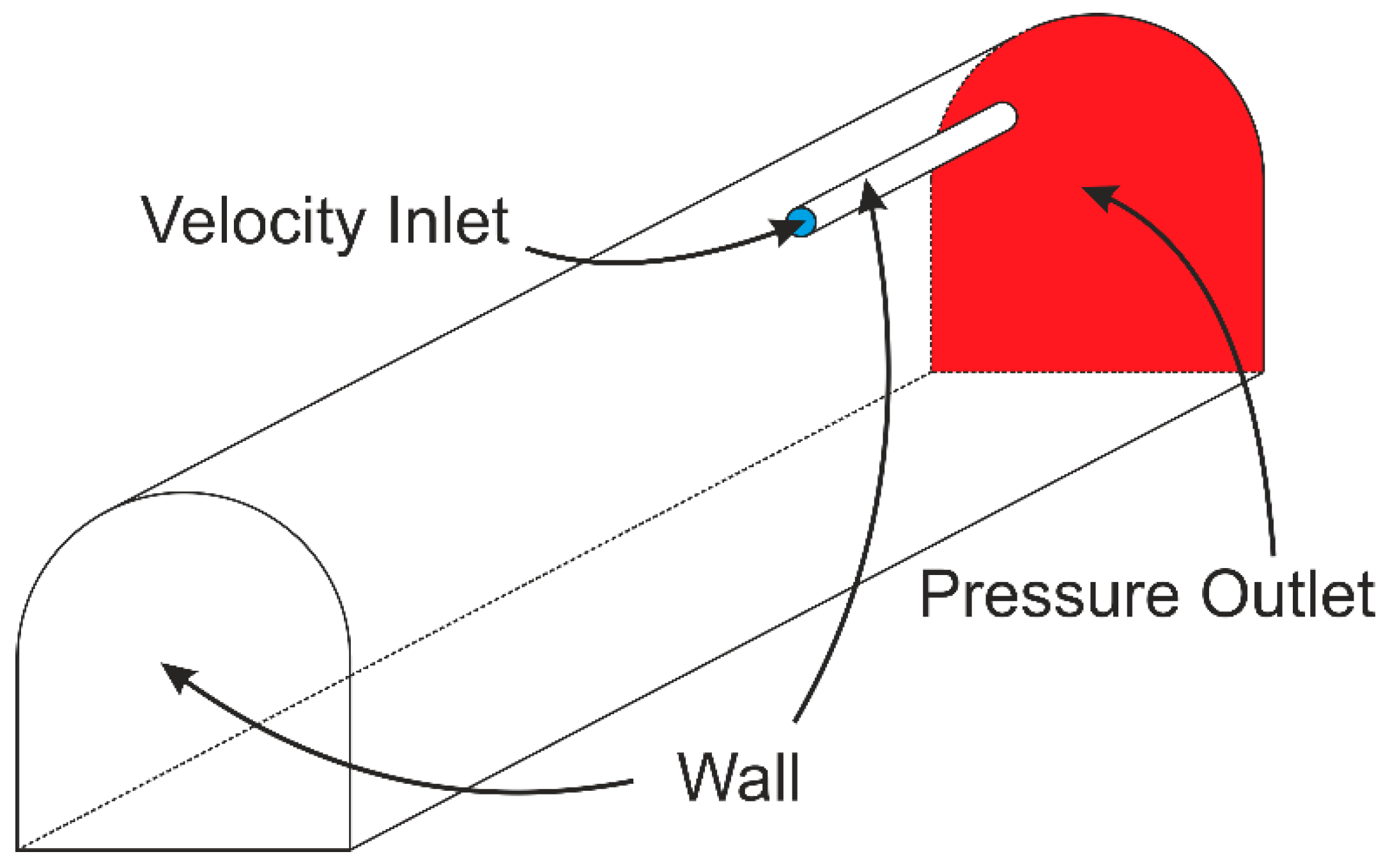
2.5. Boundary Conditions

The boundary conditions are represented in Figure 6. Walls were defined following the default criteria of the software. The inlet velocity varied from 1 to 20 m/s according to the practical values offered by Vergne (2003). The velocity at the pressure outlet was set uniform at 0 Pa, so data were in manometric pressure.

2.6. Software Configuration

In order to obtain reliable data, the following simulation parameters (

Table 2. Simulation parameters.

Turbulence Model	Realizable k-ε with Non-Equilibrium
Pressure–Velocity Coupling	SIMPLE Scheme
Transient Formulation	Second-Order Implicit
Spatial Discretization
Gradient	Green-Gauss Cell-Based
Pressure	Second Order
Momentum	Second Order
Turbulent Kinetic Energy	Second Order
Turbulent Dissipation Rate	Second Order

) were selected.

To minimize the results, errors all residuals of the simulation were set at 10⁻⁵. This fact enables us to obtain more reliable data. Also, all simulations were initialized with 0 velocity in the three components, which is more important in the mixture model simulations.

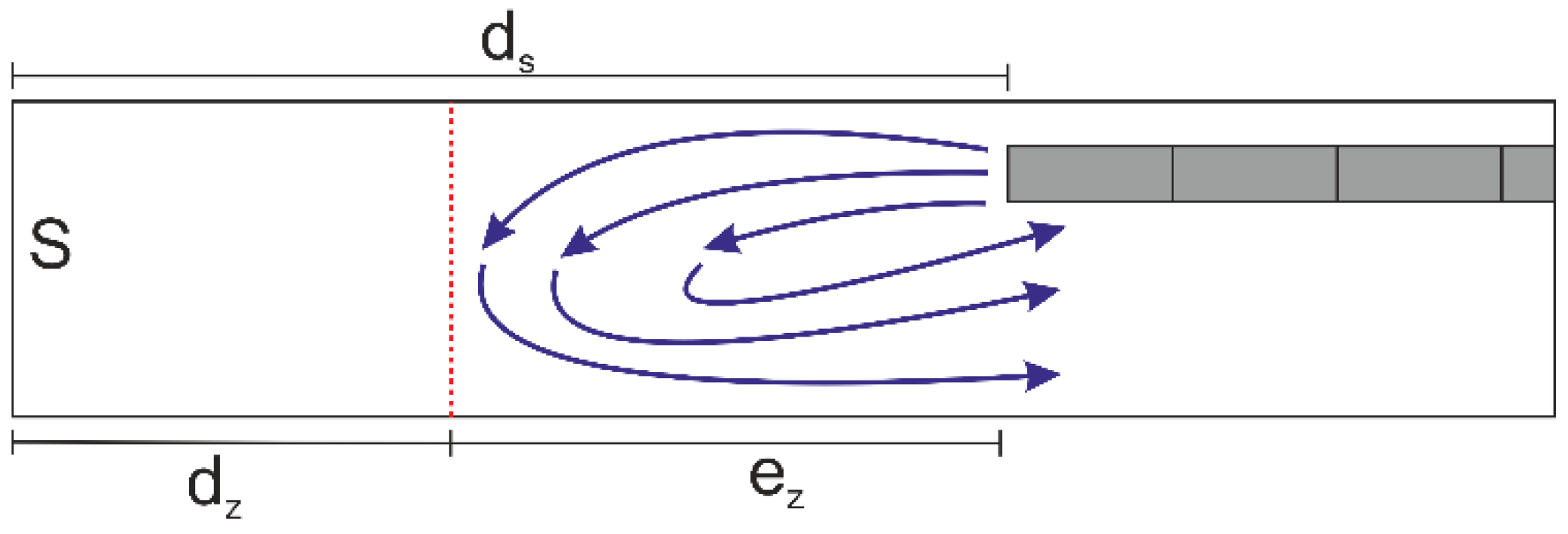
2.7. Dead Zone Delimitation

The dead zone is the area in which the ventilating flow is not capable of sweeping the blasting gases. For practical reasons, several authors and legislations have defined the dead zone as that where the air velocity is at most 0.5 m/s [19] or, less restrictively, at most 0.15 m/s [18,25]. This definition, for a long period, implies that any air clearance is still possible until the air velocity is zero. We can see in the discussion section that this definition does not fit into reality.

For this reason, two alternative methodologies were tested in order to design the dead zone, which are: (a) air jet velocity analysis through the tunnel axis; (b) analysis of the area-weighted mean vertical speed in sections transverse to the tunnel axis.

For this first method, the control surfaces 1.25 times as large as the duct diameter and coaxial with it, were generated every half meter, covering the distance between the duct and the face. In the second approach, control surfaces were generated every half meter, covering the entire section of the tunnel.

2.8. Mixture Model

A mixture model is a simplified multiphase model regularly used to simulate homogeneously mixed flows if the coupling between the phases is strong. This model was selected to monitor the concentration of a tracer gas inside the dead-end tunnel [26]. In general, the most problematic gases after blasting are CO and NO_x (NO + NO₂), of which NO₂ is the most critical. This is because NO quickly oxidizes to NO₂, which is the most toxic and diffuses with greater difficulty.

All simulations were initialized at a concentration of 5% in the volume of this gas. Different flow rates of fresh air (0% NO₂) were simulated at the inlet to compare them with the aerodynamic simulation results. Ventilation times not greater than 20 min were considered because longer re-entry times after blasting significantly reduce tunneling productivity. All simulations were conducted for scenario 4 and with fresh air duct velocities less than 20 m/s.

3. Results and Discussion

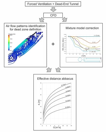
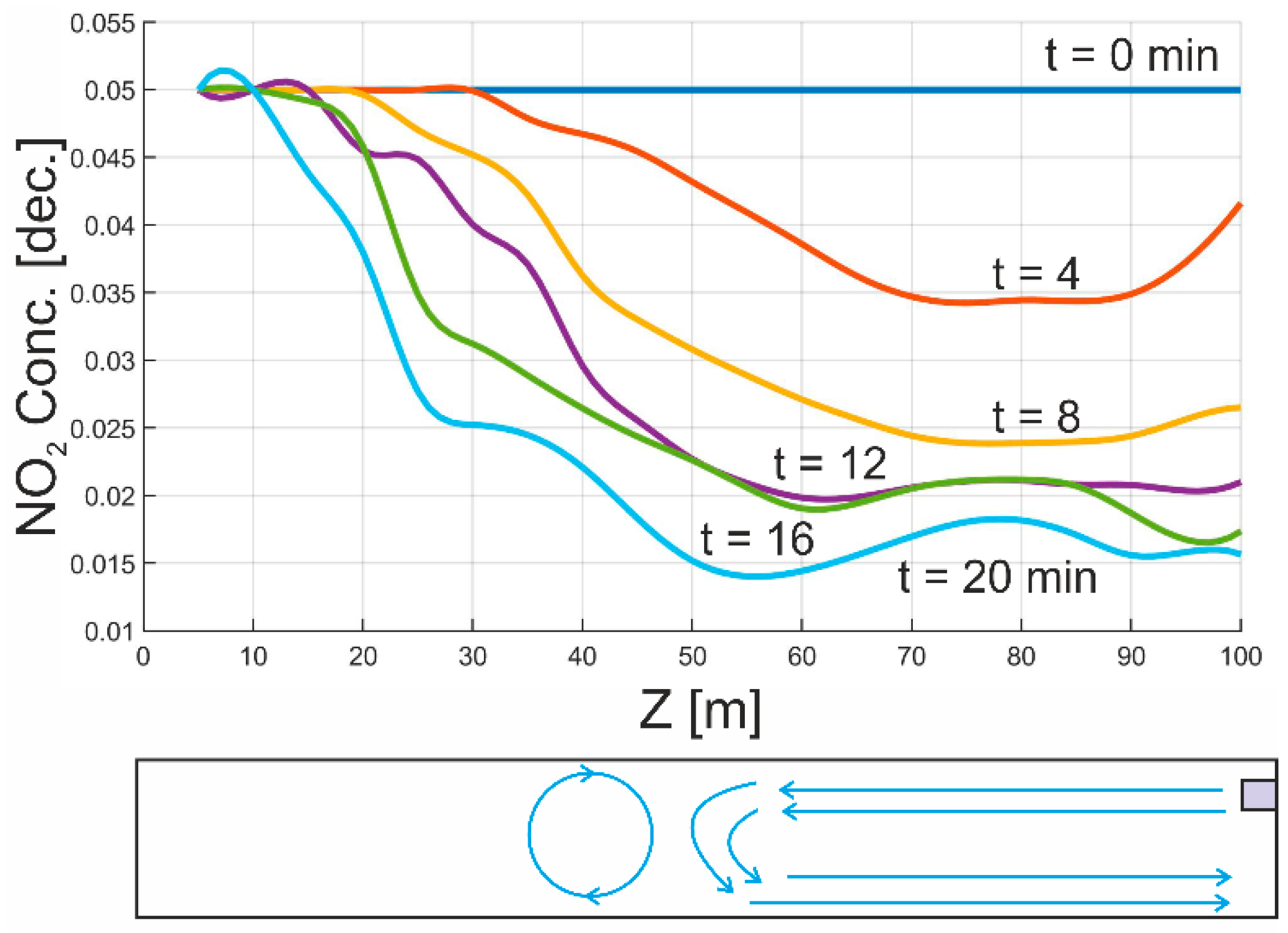
3.1. Dead Zone Delimitation and Flow Field Patterns

Figure 7 was obtained by plotting contours of the air velocity magnitude in a longitudinal plane of the tunnel, which intersects the duct. It can be observed that the air jet tends to adhere to the tunnel roof owing to the Coandă effect [27,28]. This effect increases friction and energy losses of the air jet and reduces the effective distance. Moreover, as the jet flow expands, the air velocity decreases down to values close to zero. In light of this, the first option would be to consider the effective distance as that in which the air velocity is almost zero.

Figure 8 depicts the average velocity of the air jet along the tunnel, measured in control surfaces 1.25 time as long as the duct diameter and coaxial with it. In this way, a continuum decrease in the absolute value of the air jet velocity can be observed. This curve reaches a point when velocity is almost zero and, once again, this could be defined as the beginning of the dead zone.

Figure 9 shows that most part of the air jet changes its direction, returning through the gallery before entering the dead zone. The airflow in the dead zone is also dragged by the air jet nearby and generates counter vortices due to the shear stresses. As a result, the air continually re-circulates inside the dead zone without leaving it. This phenomenon invalidates the premise of defining the dead zone as just a low-velocity region.

The analysis of the area-weighted average vertical air velocity (V_y) on control surfaces covering the entire transverse section of the tunnel is shown in Figure 10. The first phenomenon, observable at approximately 90 m from the face, was a zone of highly positive velocities. Upon analyzing the flow pattern, it can be perceived that judging from the simulation, the return flow is constricted in the lower part of the tunnel. However, at a certain moment the flow was free from the influence of the ventilation jet and filled the entire tunnel section. This phenomenon generates turbulences inside the tunnel and is responsible for this zone of mean positive vertical velocities in the simulation. Moreover, the negative mean vertical velocity observed in Figure 10 corresponds to the region where all the ventilation flow changes its direction towards the floor of the tunnel. This point is considered as the delimitation of the dead zone. In this way, we consider the limit of the dead zone where the negative vertical velocity reaches its maximum, although both approaches suggest very similar results.

Figure 11a shows the influence of the flow rate over the effective ventilation distance. According to this simulation, this distance grows rapidly for flow rates less than 1 m³/s, which are not common for mine ventilation purposes and reach a horizontal asymptote at a flow rate of about 5 m³/s. Moreover, this figure also shows a poor correlation between our expression and the legal requirements (shaded zone) for the low airflow rates and a good correlation for the large ones (horizontal asymptote). Moreover, it can be seen that the effective ventilation distance has a logarithmic relation to the flow rate. The linearization of this function allows us to assume that for common ventilation conditions, the effective distance is proportional to the logarithm of the flow rate (Figure 11b).

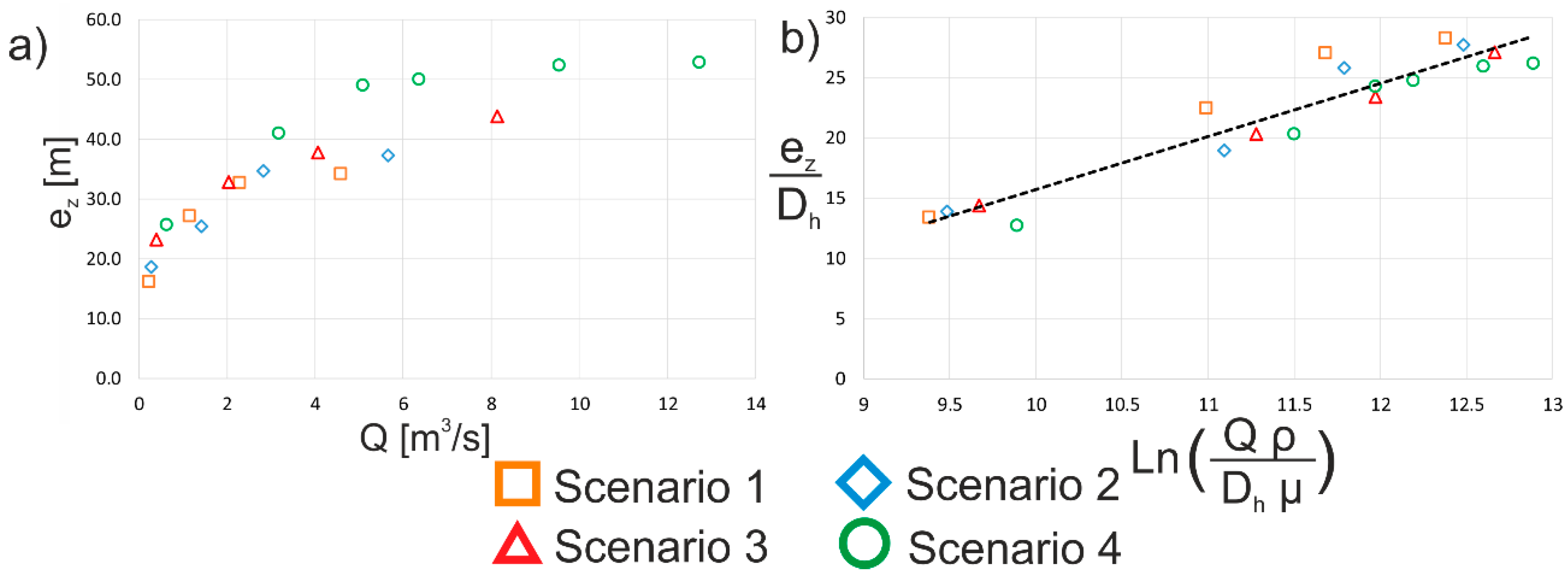
3.2. Mathematical Model for the Effective Distance

Figure 12a shows the effective distance as a function of the flow rate for each scenario. Raw data were adimensionalized using the following coefficients, where the second coefficient was derived from the Reynolds number:

$$f_1=\frac{e_z}{D_h},$$

$$f_2=\frac{Q\rho }{D_h\mu },$$

where:

• e_z: effective distance (m);
• D_h: hydraulic diameter of the tunnel section (m);
• Q: ventilation flow rate (m/s);
• ρ: air density (kg/m³);
• μ: air dynamic viscosity (Pa·s).

Figure 12b shows the transformed data according to the first dimensionless coefficient and the logarithm of the second. It was observed that if the curves were adimensionalized, they overlapped. That is to say, the solution is proportional if tunnel and duct sections remain constant. These results imply that this section alone should no longer be a parameter to study, and further work should be undertaken to study other parameters—For instance, the ratio between tunnel and duct sections. In general terms, it can be observed that the larger the tunnel section and the clean airflow rate, the longer the maximum effective distance. These results are in accordance with Feroze and Genc [29].

From the data in Figure 12b, a linear least squares (LLS) approximation was performed so that Equation (10) was obtained. This equation allows for the approximation of the effective distance as a function of the ventilation flow rate and the hydraulic diameter, which is defined as:

$$e_z=D_h\left(4.40 Ln\frac{Q\rho }{\mu D_h}-28.36\right)$$

(10)

$$D_h=\frac{4A}{P_w}$$

where:

• A: cross-sectional area of the tunnel (m²);
• P_w: perimeter of the cross-section (m).

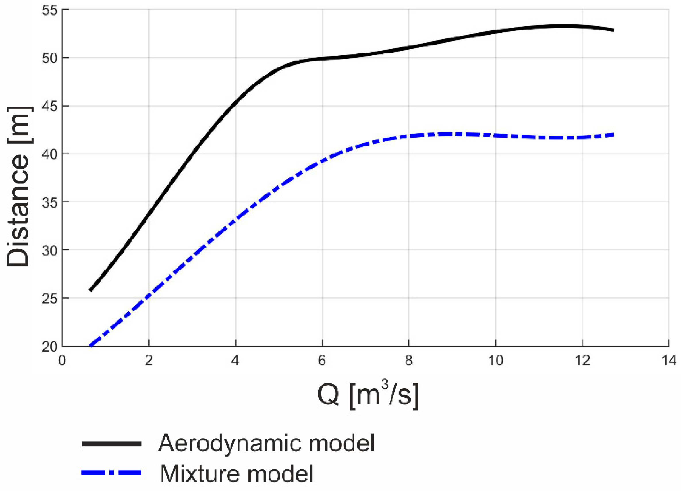
3.3. Mathematical Model Correction with the Mixture Model

The concentration of NO₂ along the tunnel axis for different ventilation times is shown in Figure 13. It can be seen that the majority of the gas dilutes in the first 12 min near the duct end (upper right part of the figure). This phenomenon corresponds to the aerodynamic sweep of NO_x by the clean air jet. Moreover, it can be observed that the clearance times are longer than 12 min. The NO_x concentration in the dead zone (left side of the figure) does not decrease significantly with the increasing ventilating time. This fact leads to the existence of a remaining concentration that can only be evacuated by diffusion. The minimum concentration remaining in the effective zone (bottom right of the figure) is the consequence of the existence of a dead zone, so the NO_x that exits this area by diffusion must cross the effective zone to leave the tunnel dead end, provoking a residual concentration of NO_x.

The diffusion mechanism is not reliable or fast enough to be taken into account for tunnel ventilation purposes, so only the distance swept by the air and not the distance cleaned by diffusion has been considered for the determination of the final effective ventilation distance corrected by the mixture model. A comparison of the data derived from the aerodynamic and the mixture model simulations is given in Figure 14. According to the mixture model, the recommended distance between the duct-end and the face is shorter than that in the aerodynamic model because in this case the time needed to evacuate the gases is taken into consideration. Moreover, if the ventilation arrangement is one that does not permit the formation of a dead zone, as could be possible in practice, the ventilating time would be shorter due to the delay imposed by NO_x diffusion inside the dead zone in the evacuation of the gases. Thus, the mixture model dilution times shown in Figure 13 are longer than the real ones as no dead zone is expected in a real tunnel ventilation situation.

Finally, upon studying the relationship between the maximum distance recommended by the mixture and the aerodynamic models (Figure 14), it can be observed that this quotient is about 0.8. Thus, a coefficient, C₁ = 0.8, was added to Equation (10) and thus Equation (11) is obtained:

$$d_s=C_1{D}_h\left(4.40Ln\frac{Q\rho }{\mathsf{\mu }{D}_h}-28.36\right)$$

(11)

It is important to keep in mind that Equation (11) does not search for the optimum distance for mine ventilation. On the contrary, it establishes a maximum duct end-to-face distance over which forced ventilation can evacuate blasting gases in a maximum of 20 min. Thus, these results do not disagree with the conventional recommendations that this distance should not to exceed ($4\sqrt{S}$–$6\sqrt{S}$), but longer clearance times should probably be expected with this expression (e.g., [19]).

Equation (11) is plotted for practical reasons in Figure 15. This graph allows for the approximation of the maximum duct end-to-face distance for some ventilation in terms of the tunnel section, clean airflow rate and ventilation time, taking into account the mixture model. Firstly, it can be observed that the larger the tunnel section, the longer the effective distance. This fact agrees with legal requirements. Furthermore, our expression takes into consideration the clean airflow rate sweeping the face, which is not considered by legal specifications. In this way, our work indicates that the larger the airflow rate, the longer the effective distance. Better correlations between legal requirements and our expression were obtained for lower airflow rates, in the case of the smaller sections. On the contrary, less disparity was achieved in the case of higher airflow rates for the larger sections.

4. Conclusions

The main aims of drivage ventilation are the evacuation of the blasting and machinery gases as well as the supply of the required air for the workers’ breathing. This type of ventilation is usually performed by means of a forcing system. In this study, a full-scale three-dimensional CFDs model of a forcing system was created to assess the ventilation performance of a dead-end gallery. The simulation was performed for different parameters, namely, tunnel section, flow rate and position with regard to the tunnel axis.

The existence of a dead zone between the duct end and the face influences the ventilation system setup. This zone has been traditionally defined as a region of reduced velocity of the air current that hinders the mixture of gases with fresh air. Our study suggests that common approaches defining the dead zone as the region in which air velocity tends to zero are not accurate. This fact is consequence of the formation counter vortexes that recirculate gases inside this zone obstructing their evacuation. Thus, although very little air renovation takes place in this zone, the gases inside it are actually in motion.

As a result of our work, we obtained an expression to approximate the maximum effective ventilating distance for some ventilation as a function of the tunnel section and the ventilation flow rate, considering a CFDs analysis with a mixture model. The equation obtained should be valid for any tunnel of similar geometry. Our calculations indicate that the maximum effective distance is larger than that suggested by traditional legal requirements, thus confirming their level of conservativism. The results obtained may assist practicing engineers in improving ventilation productivity during tunnel construction works. Future research should also consider dust when establishing an effective duct end-to-face distance for dead-end tunnel ventilation.

References

1. Sarmah, M.; Khare, P.; Baruah, B.P. Gaseous emissions during the coal mining activity and neutralizing capacity of ammonium. Water Air Soil Pollut. 2012, 223, 4795–4800. [Google Scholar] [CrossRef]
2. Osunmakinde, I.O. Towards safety from toxic gases in underground mines using wireless sensor networks and ambient intelligence. Int. J. Distrib. Sens. Netw. 2013, 2013, 159273. [Google Scholar] [CrossRef]
3. Vutukuri, V.S.; Lama, R.D. Environmental Engineering in Mines; Cambridge University Press: Cambridge, UK, 1986. [Google Scholar]
4. Borísov, S.; Klókov, M.; Gornovói, B. Labores Mineras; Mir: Moscú, Russia, 1976. [Google Scholar]
5. Novitzky, A. Ventilación de Minas; L’autor: Buenos Aires, Argentina, 1962. [Google Scholar]
6. Kissell, F. Handbook for Methane Control in Mining; DHHS (NIOSH): Pittsburg, PA, USA, 2006; Volume 131.
7. Lu, Y.; Akhtar, S.; Sasmito, A.P.; Kurnia, J.C. International Journal of Mining Science and Technology Prediction of air flow, methane, and coal dust dispersion in a room and pillar mining face. Int. J. Min. Sci. Technol. 2017, 27, 657–662. [Google Scholar]
8. Ren, T.; Wang, Z.; Cooper, G. CFD modelling of ventilation and dust flow behaviour above an underground bin and the design of an innovative dust mitigation system. Tunn. Undergr. Space Technol. 2014, 41, 241–254. [Google Scholar] [CrossRef]
9. Cheng, J.; Li, S.; Zhang, F.; Zhao, C.; Yang, S.; Ghosh, A. CFD modelling of ventilation optimization for improving mine safety in longwall working faces. J. Loss Prev. Process Ind. 2016, 40, 285–297. [Google Scholar] [CrossRef] [Green Version]
10. Lolon, S.A.; Brune, J.F.; Bogin, G.E.; Grubb, J.W.; Saki, S.A.; Juganda, A. Computational fluid dynamics simulation on the longwall gob breathing. Int. J. Min. Sci. Technol. 2017, 27, 185–189. [Google Scholar] [CrossRef]
11. Sasmito, A.P.; Kurnia, J.C.; Birgersson, E.; Mujumdar, A.S. Computational evaluation of thermal management strategies in an underground mine. Appl. Therm. Eng. 2014, 90, 1144–1150. [Google Scholar] [CrossRef]
12. Yuan, L.; Smith, A.C. Computational Fluid Dynamics Modeling of Spontaneous Heating in Longwall Gob Areas; CDC Stacks; Publick Health Publications: Atlanta, GA, USA, 2002.
13. Shi, G.Q.; Liu, M.; Wang, Y.M.; Wang, W.Z.; Wang, D.M. Computational Fluid Dynamics Simulation of Oxygen Seepage in Coal Mine Goaf with Gas Drainage. Math. Probl. Eng. 2015, 2015, 723764. [Google Scholar] [CrossRef]
14. Diego, I.; Torno, S.; Toraño, J.; Menéndez, M.; Gent, M. A practical use of CFD for ventilation of underground works. Tunn. Undergr. Space Technol. Inc. Trenchless Technol. Res. 2011, 26, 189–200. [Google Scholar] [CrossRef]
15. Toraño, J.; Torno, S.; Menéndez, M.; Gent, M. Auxiliary ventilation in mining roadways driven with roadheaders: Validated CFD modelling of dust behaviour. Tunn. Undergr. Space Technol. 2011, 26, 201–210. [Google Scholar] [CrossRef]
16. Sasmito, A.P.; Birgersson, E.; Ly, H.C.; Mujumdar, A.S. Some approaches to improve ventilation system in underground coal mines environment—A computational fluid dynamic study. Tunn. Undergr. Space Technol. 2013, 34, 82–95. [Google Scholar] [CrossRef]
17. Toraño, J.; Torno, S.; Menendez, M.; Gent, M.; Velasco, J. Models of methane behaviour in auxiliary ventilation of underground coal mining. Int. J. Coal Geol. 2009, 80, 35–43. [Google Scholar] [CrossRef]
18. Li, M.; Aminossadati, S.M.; Wu, C. Numerical simulation of air ventilation in super-large underground developments. Tunn. Undergr. Space Technol. 2016, 52, 38–43. [Google Scholar] [CrossRef]
19. Fang, Y.; Yao, Z.; Lei, S. Air flow and gas dispersion in the forced ventilation of a road tunnel during construction. Undergr. Space 2018, 4, 168–179. [Google Scholar] [CrossRef]
20. Szlazak, N.; Szlazak, J.; Tor, A.; Obracaj, A.; Borowski, M. Ventilation systems in dead end headings with coal dust and methane hazard. In Proceedings of the 30th Internetional Conferences of safety in Mines Research Institutes, Johannesburg, South Africa, 5–9 October 2003. [Google Scholar]
21. Reed, W.; Taylor, C. Factors affecting the development of mine face ventilation systems in the 20th century. In Proceedings of the Society for Mining, Metallurgy and Exploration (SME): Annual Meeting and Exhibit, Denver, CO, USA, 25–28 February 2007. [Google Scholar]
22. De La Vergne, J.; Mcintosh, S. Hard Rock Miners Handbook; Stantec: Edmonton, AB, Canada, 2000; Volume 4, ISBN 0-9687006-0-8. [Google Scholar]
23. ANSYS. ANSYS FLUENT 16.2 User’s Guide; ANSYS: Canonsburg, PA, USA, 2016. [Google Scholar]
24. López González, M.; Galdo Vega, M.; Fernández Oro, J.M.; Blanco Marigorta, E. Numerical modeling of the piston effect in longitudinal ventilation systems for subway tunnels. Tunn. Undergr. Space Technol. 2014, 40, 22–37. [Google Scholar] [CrossRef]
25. Ministry of Water Resources of the People’s Republic of China. Construction Specifications on Underground Excavation Engineering of Hydraulic Structures; China Water Power Press: Beijing, China, 2007. [Google Scholar]
26. Kurnia, J.C.; Sasmito, A.P.; Mujumdar, A.S. Simulation of a novel intermittent ventilation system for underground mines. Tunn. Undergr. Space Technol. 2014, 42, 206–215. [Google Scholar] [CrossRef]
27. Betta, V.; Cascetta, F.; Musto, M.; Rotondo, G. Numerical study of the optimization of the pitch angle of an alternative jet fan in a longitudinal tunnel ventilation system. Tunn. Undergr. Space Technol. 2009, 24, 164–172. [Google Scholar] [CrossRef]
28. Ji, J.; Fan, C.G.; Gao, Z.H.; Sun, J.H. Effects of Vertical Shaft Geometry on Natural Ventilation in Urban Road Tunnel Fires. J. Civ. Eng. Manag. 2014, 20, 466–476. [Google Scholar] [CrossRef]
29. Feroze, T.; Genc, B. Analysis of the effect of ducted fan system variables on ventilation in an empty heading using CFD. J. S. Afr. Inst. Min. Metall. 2017, 117, 157–167. [Google Scholar] [CrossRef] [Green Version]
Figure 1. Section (S), dead (dz) and effective zones (ez) for a drivage forcing ventilation system.
Energies 12 03352 g001
Figure 2. Flow chart that depicts the methodology followed.
Energies 12 03352 g002
Figure 3. Definition of the parameters. Tunnel view: Left, lateral; right, front.
Energies 12 03352 g003
Figure 4. (a) Mesh and (b) mesh quality in terms of angle criterion.
Energies 12 03352 g004
Figure 5. Mesh sensibility analysis.
Energies 12 03352 g005
Figure 6. Boundary conditions of the simulations.
Energies 12 03352 g006
Figure 7. Velocity contours of the air jet exiting the ventilation duct along the tunnel axis. The data correspond to scenario 4 and 20 m/s air velocity at the velocity inlet.
Energies 12 03352 g007
Figure 8. Jet velocity for scenario 4 and a duct velocity of 20 m/s.
Energies 12 03352 g008
Figure 9. Counter vortices formation in the dead zone.
Energies 12 03352 g009
Figure 10. Mean vertical velocity along the tunnel axis for scenario 4 and inlet velocity 20 m/s.
Energies 12 03352 g010
Figure 11. (a) Effective zone (ez) versus flow rate (Q) for scenario 4. The shaded zone indicates the recommended distance ( 4 S to 6 S ) between the duct end and the face; (b) the effective zone (ez) versus the log flow rate (Q) for scenario 4.
Energies 12 03352 g011
Figure 12. (a) Maximum effective distance (ez) versus flow rate (Q); (b) dimensionless effective distance versus the logarithm of the dimensionless effective flow rate, for the different scenarios.
Energies 12 03352 g012
Figure 13. Concentrations of NO2 inside the dead end for different ventilating times. The data correspond to scenario 4 and an air velocity of 20 m/s at the duct inlet.
Energies 12 03352 g013
Figure 14. Maximum possible duct end-to-face distance for some ventilation of the dead zone, obtained with the aerodynamic and mixture models.
Energies 12 03352 g014
Figure 15. Maximum possible duct end-to-face distance for some ventilation of the dead zone, in terms of airflow rate and tunnel section.
Energies 12 03352 g015