Abstract
A photovoltaic (PV) array is composed of several panels connected in series-parallel topology in most actual applications. However, partial shading of a PV array can dramatically reduce power generation. This paper presents a new reconfiguration method to extract more power from PV arrays under partial shade conditions. The method is designed using the effective maximum power point current and voltage of a PV panel. Its advantages involve (i) the method reconfigures the PV array without measuring the irradiance profile, and (ii) the reconfiguration is executed on the level of a PV module. Based on these two aspects, the method disperses the shade uniformly within the PV array, reducing the mismatch loss significantly and increasing power generation. The performance of the proposed method is investigated for different shade patterns and results show improved performance under partial shade conditions.
1. Introduction
With the growing demand for electrical energy and environment protection, photovoltaic (PV) systems have drawn more and more attention since they can provide renewable and clean energy [1,2]. In its application, a PV array may be partially shaded due to clouds, buildings, trees, and bird litters, etc. [3,4,5]. Under partial shade conditions, current mismatch and voltage mismatch can dramatically reduce the power generation of a PV array [6,7,8]. In particular, if shading occurs at midday, when solar irradiation is high, the shadow effect would be significant [9]. Apart from shade area, the power loss of a PV array under partial shade conditions is also related to the shade pattern and array configuration [10]. Meanwhile, the power-voltage (P-V) curve of a PV array exhibits multiple peaks, only one of which is a global maximum power point (GMPP). This increases the difficulty in maximum power point tracking (MPPT) [11]. To track the GMPP, multiple techniques have been used for MPPT, such as an artificial neural network [12], fuzzy logic control [13], the generalized pattern search method [14], and the improved pattern search method [15]. It should be noted that even when GMPP is tracked, part of the modules may not output power since the shaded modules may be short-circuited by the bypass diode [16]. As a result, the extracted power of a PV array will be lower than it can deliver [17]. Additionally, a mismatch problem can also lead to a hot-spot effect, which accelerates the degeneration of PV panels and increases the discrepancy of cell parameters. As a result, the mismatch problem is aggravated [18].
To mitigate the drawbacks of a mismatch problem, various strategies have been proposed in reported literatures. Static methods aim to decrease mismatch losses without changing the configuration of the PV array. For example, researchers have studied the effect of the configuration of the bypass diode on the PV array [19]. Furthermore, a new generation of bypass diodes with lower forward voltages are also applied to increase mismatch tolerance [20]. On the other hand, different configurations of PV arrays have also been investigated to address mismatch losses (e.g., series parallel (SP), total cross ties (TCT), and bridge link (BL) [21,22]) and have found that the TCT arrangement shows the least mismatch loss in most cases. Both of these methods can improve PV array performance under mismatch conditions, although the improvement is limited by the fixed configuration of a PV array. Multi-tracker converters are also adopted for mismatch conditions [23]. However, the high cost hinders its actual application [24].
The dynamic method reconfigures a PV array by switching the switch matrix controlled by the reconfiguration algorithm. Shade is then dispersed within the whole PV array, leading to the decrease of mismatch loss. The working condition of a PV panel is needed for design in the reconfiguration method. In this paper, a PV module, panel and array are defined as follows: A PV module is composed of a certain number of series-connected solar cells anti-parallel connected with a bypass diode. Several series-connected PV modules are packaged to form a PV panel. Finally, a PV array is formed by parallel-connected PV strings consisting of series-connected PV panels. Some of the most commonly used variables to describe the working condition of a PV panel include irradiance, temperature and electrical parameters [25]. In Reference [26], irradiance of a PV panel is used to reconfigure the PV array. The irradiance is calculated using the short-circuit current and temperature of the PV panel. However, the method is only suitable for situations with uniform irradiance patterns. This can be explained by Figure 1, showing the schematic diagram of PV panel subjected to different irradiance patterns. As shown in Figure 1, an irradiance pattern may be divided into a uniform (a,b) or non-uniform irradiance pattern (c). Obviously, the irradiance pattern of a PV panel can be substituted by an irradiance value only when the irradiance pattern is uniform. In Reference [27], the reconfiguration method is designed using the irradiance of each PV cell. Compared to Reference [26], the method outlined in Reference [27] is also suitable for non-uniform irradiance conditions. However, the method needs the irradiance of each PV cell, which is hard to acquire in actual applications. The other category of reconfiguration method uses the electrical parameters of a PV panel to reconfigure the PV array. In Reference [24], short-circuit current is used to design the reconfiguration method. As shown in Figure 1, a PV panel is composed of three modules. Each module is anti-parallel connected with a bypass diode. Under non-uniform irradiance patterns, the measured short-circuit current of a PV panel is the maximum short-circuit current of its three PV modules. Thus, the method described in Reference [24] is also suitable for uniform irradiance patterns. In Reference [17], the area enclosed between the power-current (P-I) curve and the I-axis of the PV panel is used to design the reconfiguration algorithm. An advantage of this algorithm is that it is independent of the irradiance pattern. However, the method considers all modules in the same PV panel as a whole. Under non-uniform irradiance pattern conditions, the irradiance patterns of the PV modules are different. Thus, reconfiguration of a PV array on the module level (rather than the panel level) can provide better performance. In Reference [28], the MPP current and voltage of the PV modules are used to reconfigure the PV array. However, the reconfiguration of a PV array with more than two strings is not given.
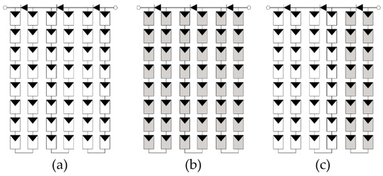
Figure 1.
(a) Schematic diagram of a PV panel without shading; (b) a PV panel with a uniform irradiance pattern; and (c) a PV panel with a non-uniform irradiance pattern.
Based on the analyses above, three factors must be considered in designing the reconfiguration method for a PV array composed of panels: (i) The method should be suitable for any irradiance pattern, i.e., uniform and non-uniform irradiance patterns; (ii) the reconfiguration should be carried out at the module level; and (iii) the method can be easily applied to a PV array with any number of strings. In this research, a new method is proposed to reconfigure the partially shaded PV array with SP topology, satisfying all three factors. The performance of the proposed method is investigated for different shade patterns and the results show better performance compared with the reconfiguration methods reviewed.
2. Effective MPP
2.1. Power Output of a PV Panel Under Partially-Shaded Conditions
The output characteristics of a partially shaded PV array can be modeled based on the equivalent circuit of a PV cell, such as a one diode model or a two diode model. In this paper, a one diode model is adopted since the accuracy is enough and the expression is simple [29,30,31]. The equivalent circuit of a one diode model is shown in Figure 2.
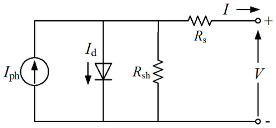
Figure 2.
Equivalent circuit of a PV cell (one diode model).
According to the equivalent circuit of a PV cell, the output current of a PV cell can be written as:
where is the photo-generated current, is the diode reverse saturation current, and are the series and parallel resistance, respectively, is the thermal voltage of the PV cell, T is the cell temperature, is the electron charge, is Boltzmann’s constant and a is the diode ideality factor. According to Equation (1), the output characteristics of a PV cell is simulated in Matlab and shown in Figure 3.
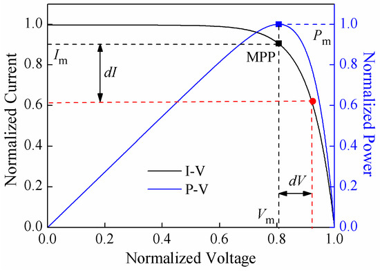
Figure 3.
I-V and P-V curves of a PV cell.
It can be found that the P-V curve exhibits one power peak at the MPP voltage, . The corresponding current is MPP current, . When all of the PV panels operate at their MPP, the absolute maximum power of the PV array is:
where is the number of strings, and is the number of PV panels in a string. The absolute maximum power is the maximum power that a PV array can output, i.e., the mismatch loss is zero. The absolute maximum power can be acquired only when a PV array is subjected to uniform irradiance.
Under mismatch conditions, the operating point of a PV panel will deviate from its MPP. Supposing the MPP voltage and current deviation is and , respectively, then the actual power output is:
Since the purpose of reconfiguration is to extract the maximum power from a PV array, the current mismatch and voltage mismatch is actually the mismatch of and among PV panels. Therefore, MPP current and voltage are used to design the reconfiguration method.
2.2. Effective MPP for Reconfiguration
Since a PV panel is composed of several modules, the irradiance of modules in the same panel may be different under partially shaded conditions. In this case, the P-V curve of the PV panel exhibits multiple MPPs. Only effective MPP (EMPP) is selected for reconfiguration. EMPP refers to global MPP (GMPP) and local MPP (LMPP) with current larger than the GMPP current. Suppose a PV panel is composed of three modules, M1, M2 and M3, and irradiance of the three modules satisfy: > > , then the P-I curve of such a PV panel is shown in Figure 4. We can find that the P-I curve exhibits three MPPs, i.e., GMPP, LMPP1 and LMPP2, where the subscript 1 and 2 refer to the first and second LMPP respectively. In Figure 4, EMPP refers to GMPP and LMPP2.
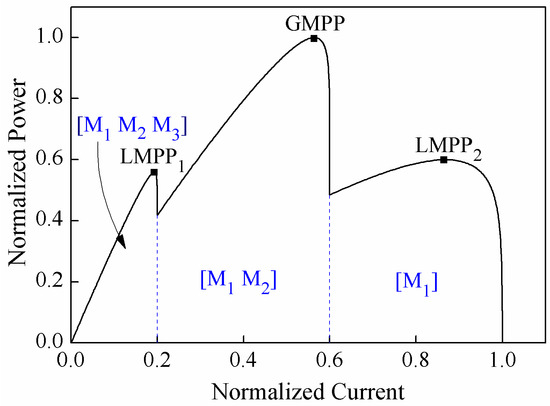
Figure 4.
P-I curve of a PV panel under non-uniform irradiation.
The reason for using EMPPs to execute the reconfiguration is explained as follows. On the one hand, reconfiguration is executed on the level of the module if the EMPP is used for reconfiguration. As shown in Figure 4, different MPPs correspond to different numbers of effective modules. Here, the effective module is the module that is not short-circuited by a bypass diode. For example, if a PV string operates at GMPP in Figure 4, M3 is bypassed and cannot output power since its short-circuit current is smaller than the string current. Therefore, M1 and M2 are effective modules. Similarly, if a PV string operates at LMPP1 and LMPP2, effective modules are M1, M2, M3 and M1 respectively.
On the other hand, using EMPP for reconfiguration is beneficial for minimizing the total mismatch of PV panels. The optimal situation is that a PV panel can operate at GMPP. However, it is not necessarily the best choice for reconfiguration since the total mismatch may not be minimized. The power of a PV string can be expressed as:
where is the power of the i-th PV panel, is the power of PV module, and is the number of modules in a PV panel. = 1 if the short-circuit current of PV module, , is larger than the string current. Otherwise, = 0. For the situation in Figure 4, the string power is:
where > > . Though is larger than , the current mismatch of other panels is also larger when the string current equals to . Thus, LMPP2 may be a better choice. Likewise, LMPP with a current smaller than the current of GMPP, e.g., LMPP1 in Figure 4, should be discarded because there is a larger current mismatch when the string operates at .
3. Proposed Reconfiguration Algorithm
3.1. GMPP Power of Partially Shaded PV Array
The power output of a PV array with SP topology is:
where is the current of a PV string, and is the voltage of the PV array. Under non-uniform irradiance conditions, is different from , . The notation represents the MPP voltage of a PV string, where the superscript denotes the number of effective modules in the string and the subscript j represents the j-th string. If is satisfied, the relationship between and can be sorted into two categories, which is illustrated by P-V curves of a PV array and its two strings, as shown in Figure 5. PV string 1 is partially shaded. Specifically, it receives an irradiation profile consisting of two irradiance levels. Thus, the P-V curve of string 1 exhibits two MPPs: MPP11 and MPP12 in Figure 5. On the contrary, PV string 2 is uniformly illuminated and therefore the P-V curve of string 2 exhibits only one MPP: MPP2 in Figure 5.
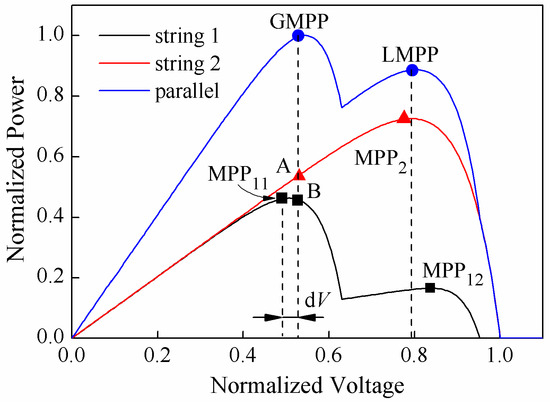
Figure 5.
Relationship between the PV array and string MPP.
In the case depicted in Figure 5, LMPP can be considered as the superposition of MPP12 and MPP2, which is the case when is satisfied. In this scenario, the difference between and is small [32]. Thus, the power of the PV array can be approximately expressed as:
where . In each string, the current of MPP corresponding to effective modules is approximately equal to the minimum of all effective modules [33]. Therefore, the maximum power is:
where , is the number of effective modules, and approximately equals the minimum EMPP current of panels in i-th string. Therefore, to maximize the power output of PV array, i.e., to get the optimal configuration, the maximized power output is:
From the analysis above, we can conclude that the MPP voltage difference can be neglected if the number of effective modules in all strings is the same. Therefore, the optimal configuration can be acquired as long as is maximized, which corresponds to the minimum current mismatch.
On the contrary, GMPP is the superposition of MPP11 and MPP2, which corresponds to the case when is not satisfied. We may find that the voltage mismatch between string 1 and string 2 cannot be neglected since the voltage different between and is very large. Meanwhile, as depicted in Figure 5, the voltage difference between and is small due to the sharp decrease of the P-V curve on the right side of MPP11. This indicates that the difference in the number of effective modules for different strings should be as small as possible. Therefore, the reconfiguration of a PV array can be executed in two steps: (i) Minimize the difference in effective module numbers among different strings; and (ii) maximize on the basis of (i).
3.2. Proposed Reconfiguration Algorithm
Based on the analysis above, the detailed reconfiguration algorithm for a PV array with SP topology is shown as follows:
Step 1: Trace the I-V curve of PV panels by a suitably controlled DC/DC converter. Based on the recorded data, calculate the P-V curve by the linear interpolation method and find all EMPPs of the PV panel. EMPP voltages are simplified as the number of effective modules. Meanwhile, the interpolated data is also used to calculate the I-V curve of a PV string and array [17].
Step 2: Determine the possible configurations of a PV array from the first string to the last string, successively.
Sub-step 2.1: For each PV panel, all recorded EMPPs are ranked in descending order based on their power. Take the first EMPP voltage and current of each panel to execute reconfiguration. Rank the EMPP currents in descending order, forming the EMPP current vector . Correspondingly, EMPP voltages should also be ranked based on the order of EMPP currents to acquire the EMPP voltage vector . Here, is the number of PV panels connected into the PV array.
Sub-step 2.2: Calculate the reference voltage of the i-th string () and determine the number of effective module in the string. For the i-th string, the reference voltage is:
where , is the number of PV panels in a string. Supposing rounds to the nearest integer towards minus infinity and , the number of effective modules in the i-th string is determined as follows:
Sub-step 2.3: Determine the configuration of the i-th string. If the sum of the first f elements in equals to , i.e., , then the first f modules form the i-th string and the other modules form the rest of the strings. Otherwise, find the first f elements that satisfy and . The first modules are part of the i-th string . Other elements in are divided into categories. Supposing equals to 2, then the elements are in two categories, and . The elements in is j, where j = 1 or 2. Calculate the difference between and , i.e., . Select the first and elements in and to form EMPP voltage combinations . These elements satisfy , and the i-th string is the combination of and . After determining all panels in the i-th string, can be easily determined as the minimum EMPP current.
Sub-step 2.4: Delete the elements in S1 from the EMPP voltage and current vector. Return to sub-step 2.1 to determine the (i+1)-th string until the last string.
Step 3: Calculate the GMPP power, , of the reconfigured PV array. If decreases compared with the final configuration in the last iteration, stop the reconfiguration process—the configuration determined in the last iteration is the optimal configuration. Otherwise, update the EMPP with minimum current based on the following EMPP replacement rule and return to step 2:
1. If the PV panel with minimum MPP current only has one EMPP and EMPP voltage is 1, disconnect the PV panel from PV array.
2. If the PV panel with minimum MPP current only has one EMPP and EMPP voltage is larger than 1, the EMPP voltage is replaced with .
3. If the PV panel with minimum EMPP current has more than one EMPP, use the EMPP with the larger current to replace this EMPP.
The flowchart of the proposed reconfiguration algorithm is shown in Figure 6.
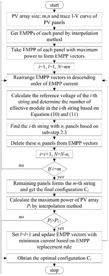
Figure 6.
Flowchart of the proposed reconfiguration algorithm.
4. Simulation Results and Discussion
The performance of the proposed algorithm was evaluated for different shade patterns in Matlab/Simulink. The PV array consisted of 10 panels, with each panel being composed of three series-connected solar modules. One bypass diode was anti-paralleled with the PV module. Each string was series-connected with a blocking diode to prevent current back flow. All switches were assumed to be ideal. The PV panels were interconnected through a reconfiguration switch matrix. By turning specific switches on and off, the corresponding panel was connected or disconnected from the PV array. Meanwhile, all of the PV panels were connected with measurement devices through measurement switches. When a specific switch was active, the corresponding panel was connected with its measurement device and, therefore, the I-V characteristics of the panel were measured. The complete simulated reconfiguration system is depicted in Figure 7. The reconfiguration algorithm was executed by an S-function in the simulation. Note that in actual applications, the reconfiguration algorithm could be executed using digital processors like DSP or FPGA. When an updated measure of the panels’ I-V characteristics was required, the controller sequentially controlled each panel to be disconnected from the array (by the reconfiguration switch matrix) and connected to the measuring device via the measurement switches. After a complete scan was performed, the optimal configuration was determined by the reconfiguration algorithm. The optimal configuration was then acquired by controlling the reconfiguration switches. In this paper, Cori and CEMPP are defined as the original configuration and the reconfigured configuration by proposed method respectively. Meanwhile, to test its validity, CEMPP was also compared with the optimized configuration, i.e., Copt, in Reference [17]. The reconfiguration efficiency was defined to quantify the performance of the reconfiguration algorithm as follows:
where is the GMPP power of the PV array without reconfiguration and is the GMPP power of the PV array after reconfiguration.
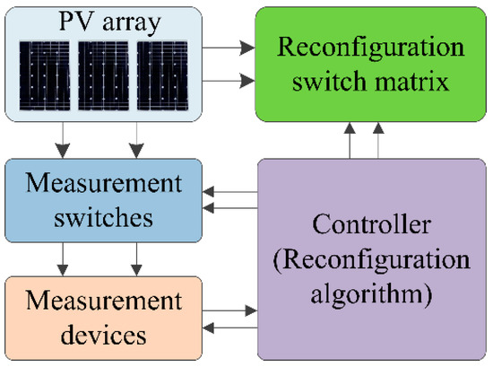
Figure 7.
Diagram of the reconfiguration system.
4.1. Case 1
A PV array composed of two strings with an irradiance pattern, as shown in Figure 8, is considered in this case. The first four panels in the first string, S1, receive uniform irradiance of 700 , while the first four panels in the second string receive non-uniform irradiance of 200 and 1000 . The temperature of the PV modules subjected to 200, 700 and 1000 is assumed to be 20, 35 and 44 , respectively. The ten panels are labeled as N1 to N10. Note that Section 3 provides a detailed explanation of the reconfiguration steps, explicating the algorithm.
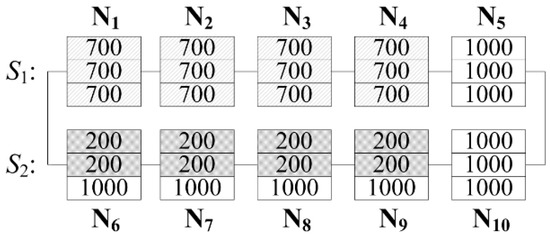
Figure 8.
Irradiance pattern of Case 1.
4.1.1. EMPPs for Reconfiguration
The first step was to determine the EMPPs of all of the panels. As shown in Figure 8, there are three types of irradiance patterns for PV panels: Uniform irradiance of 1000 (Type 1), uniform irradiance of 700 (Type 2) and non-uniform irradiance with both 200 and 1000 (Type 3). P-V curves of three types of PV panels are shown in Figure 9. For Type 1 and 2, there is only one MPP on the P-V curve. Therefore, this MPP is the EMPP. For Type 3, the P-V curve exhibits two MPPs. According to the definition of EMPP, GMPP is the only EMPP since the current of LMPP is smaller than that of GMPP. The EMPP voltage and current of Type 1, 2, 3 are 3, 3, 1 and 1.52, 1.48, 1.05, respectively. Thus, the EMPP current and voltage vector can be acquired as: = [1.52 1.52 1.48 1.48 1.48 1.48 1.05 1.05 1.05 1.05], = [3 3 1 1 1 1 3 3 3 3].
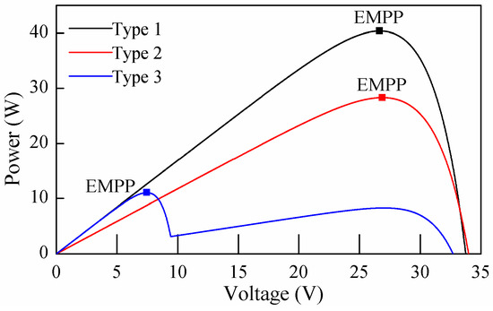
Figure 9.
P-V curve of three types of PV panel.
4.1.2. Determination of Possible Configurations
With reference to Steps 2 and 3, the process used to determine possible configurations is shown in Figure 10. In the first iteration, the reference voltage and the number of effective modules for S1 wats calculated as 11. Then the configuration of the PV array was determined following sub-step 2.3. Since = 10 < and = 13 > , k was 7 and the first four panels formed part of the first string . The rest of the panels were divided into three categories: : [1 1], T2: [] and : [3 3 3 3]. The difference between and was calculated as = 3. This meant three effective modules were needed to form S1b. The possible combination could have been {1,1,1} or {3}. Only {3} could be acquired in this case. Thus, the first string configuration was {N10, N5, N6, N7, N1} with a voltage vector [3 3 1 1 3], with the rest of the panels forming the other string. Using the interpolation method, we calculated the maximum power of the configuration, C1, as 215.2 W.
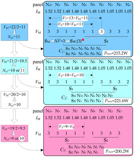
Figure 10.
Determination of possible configurations in Case 1.
In the second iteration, the EMPP voltage of N4 was changed to 2 in accordance with the EMPP replacement rule. The reference voltage of S1 was 10.5. Thus, the number of effective modules was 10 or 11. If = 11 was selected, the final configuration was the same as C1. Therefore, the determination of a possible configuration was given when = 10 was considered. Following sub-step 2.3, C2 was determined and its maximum power calculated as 221.6W. Since the maximum power of C2 was larger than that of C1, the reconfiguration continues.
In the subsequent iteration, the EMPP voltage of N4 was changed as 1. The reference voltage and the number of effective modules was calculated as 10. Since the EMPP current vector was not changed, the final configuration was the same as C2. Then, according to the EMPP replacement rule, N4 was disconnected from the PV array. By applying the same step above, C3 was determined and the maximum power of C3 was calculated as 200.2 W. Since the maximum power of C3 was smaller than that of C2, the reconfiguration process stopped, and C2 was selected as the optimal configuration for its maximum power among C1, C2 and C3.
The final configurations of CEMPP and Copt are shown in Figure 11; the corresponding P-V curves are compared in Figure 12. The global power point corresponding to Cori, CEMPP and Copt is observed at 188.3 W, 221.6 W and 195.8 W, respectively. The reconfiguration efficiency of CEMPP and Copt is 17.68% and 3.98%, respectively. The improvement of CEMPP compared with Copt is attributed to a much smaller current mismatch in CEMPP. For Type 3, GMPP was the only EMPP, which meant only the module subjected to 1000 W/m2 was an effective module. For Type 1 and 2, all of the modules were effective. In CEMPP and Copt, the number of effective modules in S1 and S2 was the same, i.e., 10 and 12. However, the current mismatch of CEMPP and Copt were different. Since the reconfiguration using the proposed method was on the level of the PV module, the effective modules with the same irradiance were connected to the same string. This minimized the current mismatch. On the contrary, effective modules with different irradiances were connected in the same string using the method in Reference [17], causing significant current mismatch of modules with irradiance of 1000 W/m2.
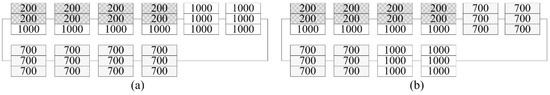
Figure 11.
(a) Optimized configuration CEMPP and (b) optimized configuration Copt.
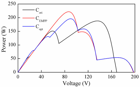
Figure 12.
P-V curve of a PV array before and after reconfiguration.
4.2. Case 2
For case 2, the primary and optimized configurations are shown in Figure 13a,b, respectively. In this case, the first two panels in both strings received an irradiance of 600 W/m2 and the temperature of these panels was assumed to be 32 . As shown in Figure 13b, the proposed and reference method provide the same result. According to the P-V curves shown in Figure 14, the GMPP values obtained for Cori and CEMPP (Copt) are 271 W and 325 W, respectively, which means 19.93% extra power is acquired.
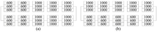
Figure 13.
(a) Primary configuration Cori and (b) optimized configuration CEMPP (Copt).
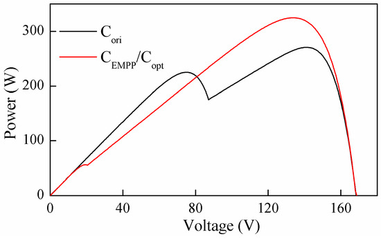
Figure 14.
P-V curve of a PV array before and after reconfiguration.
4.3. Case 3
For this case, the primary and optimized configurations are shown in Figure 15. The P-V curve of the PV array with a different configuration is shown in Figure 16. The global power point corresponding to Cori, CEMPP and Copt is observed at 226.5 W, 261.9 W and 253.0 W, respectively. Therefore, the reconfiguration efficiency of CEMPP and Copt are 15.6% and 11.7%, respectively. Also in this case, the proposed method had a better performance compared with the reference method. The improvement can be illustrated based on the difference between CEMPP and Copt, shown in Figure 15b,c, respectively. In both configurations, two PV panels subjected to uniform irradiance of 200 W/m2 were disconnected from the PV array. In the eight remaining panels, the module with an irradiance of 1000 W/m2 was the effective module. In CEMPP, 20 effective modules were evenly allocated in two strings, i.e., 10 effective modules per string. On the contrary, the number of effective modules for Copt in two strings was 11 and 9, leading to higher voltage mismatch and therefore lower power output.
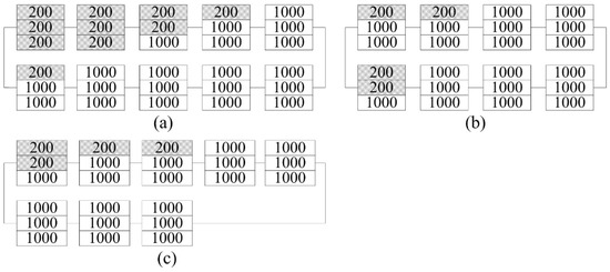
Figure 15.
(a) Primary configuration Cori; (b) optimized configuration CEMPP; and (c) optimized configuration Copt.
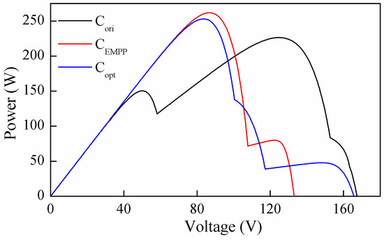
Figure 16.
P-V curve of a PV array before and after reconfiguration.
4.4. Case 4
A PV array with three strings was considered in case 4. The irradiance pattern is shown in Figure 17a. The temperature of the PV module subjected to 300 was assumed to be 23 . The PV array reconfigured by the proposed method and the reference method are shown in Figure 17a,b. The P-V curves of the PV array before and after reconfiguration are compared in Figure 18. According to the P-V curves, CEMPP and Copt increases the power output from 467.8 W to 524.9 W and 508.7 W, respectively, corresponding to the reconfiguration efficiency of 12.21% and 8.74%, respectively.
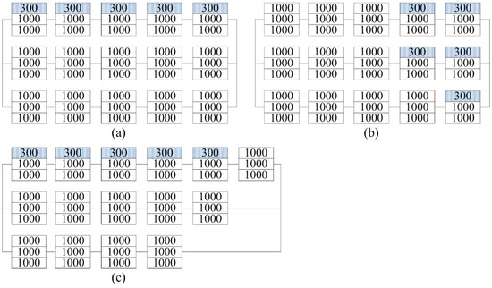
Figure 17.
(a) Primary configuration Cori; (b) optimized configuration CEMPP; and (c) optimized configuration Copt.
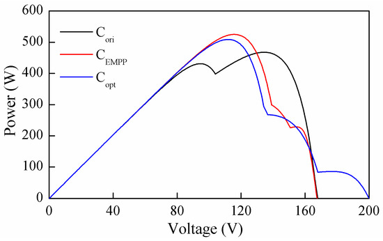
Figure 18.
P-V curve of a PV array before and after reconfiguration.
4.5. Summary of the Simulation Study
The performance of the reconfiguration algorithm can be measured by two parameters: Reconfiguration efficiency and reconfiguration time. Reconfiguration efficiency is an important parameter since the main purpose of reconfiguration is to maximize the power generation of a shaded PV array. In the four cases, both the proposed and reference algorithms increased the power output. However, the proposed algorithm outperformed the reference algorithm in cases 1, 3 and 4 and showed the same performance in case 2. Correspondingly, the reconfiguration efficiency of the proposed algorithm was 13.7%, 3.9% and 3.47% higher than that of the reference algorithm in case 1, 3 and 4, respectively. Therefore, the proposed algorithm is able to extract more power from a partially shaded PV array, leading to greater power saving and more income.
Reconfiguration time also needs to be evaluated for the reconfiguration algorithm. The larger the time needed for the reconfiguration, the lower the frequency of reconfigurations and, consequently, the higher the probability of missing the possibility of adapting the module connections to the moving shadows in time. The reconfiguration time for the four simulation cases were 2.91 s, 2.78 s, 3.09 s and 3.88 s, respectively. The much longer reconfiguration time of case 4 compared with the other three cases was mainly attributed to more panels in case 4. From the results we can find that the proposed algorithm is suitable for cases where the shadow is caused by stationary objects, such as trees, buildings, poles and moving objects with very slow speed, such as moving clouds caused by wind with low speed.
5. Conclusions
In this paper, a new reconfiguration algorithm is proposed to maximize the power generation of a PV array with SP topology under partial shade conditions. Based on the derived mathematical expression of output power generated by a partially shaded PV array, we select the EMPP voltage and current of the PV panel to design the reconfiguration algorithm. This ensures that the reconfiguration is on the module level rather than the panel level, which can reduce the current mismatch and voltage mismatch as much as possible. According to the analysis, the current mismatch can be minimized by maximizing the sum of minimum EMPP current in each string. Furthermore, the voltage mismatch can be minimized by minimizing the difference of the effective module numbers of different strings. The performance of the proposed algorithm is tested using four shade patterns in Matlab/Simulink. The proposed algorithm shows higher or equal reconfiguration efficiency than the reference algorithm. Considering the reconfiguration time, the proposed algorithm will likely be a suitable option for extracting more power from partially shaded PV arrays in situations where the shadow does not change quickly.
Author Contributions
Y.W. provided the guidance and supervision. X.L. implemented the main research and wrote the paper.
Funding
This research received no external funding.
Conflicts of Interest
The authors declare no conflict of interest.
References
- Bizon, N. Global extremum seeking control of the power generated by a photovoltaic array under partially shaded conditions. Energy Convers. Manag. 2016, 109, 71–85. [Google Scholar] [CrossRef]
- Rakesh, N.; Madhavaram, T.V. Performance enhancement of partially shaded solar PV array using novel shade dispersion technique. Front. Energy 2016, 10, 227–239. [Google Scholar] [CrossRef]
- Yadav, A.S.; Pachauri, R.K.; Chauhan, Y.K.; Choudhury, S.; Singh, R. Performance enhancement of partially shaded PV array using novel shade dispersion effect on magic-square puzzle configuration. Sol. Energy 2017, 144, 780–797. [Google Scholar] [CrossRef]
- Ngoc, T.N.; Phung, Q.N.; Tung, L.N.; Sanseverino, E.R.; Romano, P.; Viola, F. Increasing efficiency of photovoltaic systems under non-homogeneous solar irradiation using improved dynamic programming methods. Sol. Energy 2017, 150, 325–334. [Google Scholar] [CrossRef]
- Pareek, S.; Dahiya, R. Enhanced power generation of partial shaded photovoltaic fields by forecasting the interconnection of modules. Energy 2016, 95, 561–572. [Google Scholar] [CrossRef]
- Gokmena, N.; Karatepea, E.; Silvestre, S.; Celik, B.; Ortega, P. An efficient fault diagnosis method for PV systems based on operating voltage-window. Energy Convers. Manag. 2013, 73, 350–360. [Google Scholar] [CrossRef]
- Tadj, M.; Benmouiza, K.; Cheknane, A.; Silvestre, S. Improving the performance of PV systems by faults detection using GISTEL approach. Energy Convers. Manag. 2014, 80, 298–304. [Google Scholar] [CrossRef]
- Dolara, A.; Lazaroiu, G.C.; Leva, S.; Manzolini, G. Experimental investigation of partial shading scenarios on PV (photovoltaic) modules. Energy 2013, 55, 466–475. [Google Scholar] [CrossRef]
- Cotana, F.; Rossi, F.; Nicolini, A. Evaluation and optimization of an innovative low-cost photovoltaic solar concentrator. Int. J. Photoenergy 2011, 2011, 843209. [Google Scholar] [CrossRef]
- Madhusudanan, G.; Senthilkumar, S.; Anand, I.; Sanjeevikumar, P. A shade dispersion scheme using Latin square arrangement to enhance power production in solar photovoltaic array under partial shading conditions. J. Renew. Sustain. Energy 2016, 10, 063503. [Google Scholar] [CrossRef]
- Bastidas-Rodriguez, J.D.; Franco, E.; Petrone, G.; Ramos-Paja, C.A.; Spagnuolo, G. Maximum power point tracking architectures for photovoltaic systems in mismatching conditions: A review. IET Power Electron. 2014, 7, 1396–1413. [Google Scholar] [CrossRef]
- Messalti, S.; Harrag, A.; Loukriz, A. A new variable step size neural networks {MPPT} controller: Review, simulation and hardware implementation. Renew. Sustain. Energy Rev. 2017, 68, 221–233. [Google Scholar] [CrossRef]
- Liu, C.L.; Chen, J.H.; Liu, Y.H.; Yang, Z.Z. An asymmetrical Fuzzy-Logic-Control-Based MPPT algorithm for photovoltaic systems. Energies 2014, 7, 2177–2193. [Google Scholar] [CrossRef]
- Yaqoob-Javed, M.; Faisal-Murtaza, A.; Ling, Q.; Qamar, S.; Majid-Gulzar, A. A novel MPPT design using generalized pattern search for partial shading. Energy Build. 2016, 133, 59–69. [Google Scholar] [CrossRef]
- Tobón, A.; Peláez-Restrepo, J.; Villegas-Ceballos, J.P.; Serna-Garcés, S.I.; Herrera, J.; Ibeas, A. Maximum power point tracking of photovoltaic panels by using improved pattern search methods. Energies 2017, 10, 1316. [Google Scholar] [CrossRef]
- Teo, J.C.; Tan, R.H.G.; Mok, V.H.; Ramachandaramurthy, V.K.; Tan, C. Impact of partial shading on the P-V characteristics and the maximum power of a photovoltaic string. Energies 2018, 11, 1860. [Google Scholar] [CrossRef]
- Balato, M.; Costanzo, L.; Vitelli, M. Series-Parallel PV array re-configuration: Maximization of the extraction of energy and much more. Appl. Energy 2015, 159, 145–160. [Google Scholar] [CrossRef]
- Geisemeyern, I.; Fertig, F.; Warta, W.; Rein, S.; Schubert, M.C. Prediction of silicon PV module temperature for hot spots and worst case partial shading situations using spatially resolved lock-in thermography. Sol. Energy Mat. Sol. Cells 2014, 120, 259–269. [Google Scholar] [CrossRef]
- Silvestre, S.; Boronat, A.; Chouder, A. Study of bypass diodes configuration on PV modules. Appl. Energy 2009, 86, 1632–1640. [Google Scholar] [CrossRef]
- Pannebakker, B.B.; de Waal, A.C.; van Sark, W.G.J.H.M. Photovoltaics in the shade: one bypass diode per solar cell revisited. Prog. Photovolt. 2017, 25, 836–849. [Google Scholar] [CrossRef]
- Pareeka, S.; Chaturvedib, N.; Dahiya, R. Optimal interconnections to address partial shading losses in solar photovoltaic arrays. Sol. Energy 2017, 155, 537–551. [Google Scholar] [CrossRef]
- El-Dein, M.Z.S.; Kazerani, M.; Salama, M.M.A. An optimal total cross tied interconnection for reducing mismatch losses in photovoltaic arrays. IEEE Trans. Sustain. Energy 2013, 4, 99–107. [Google Scholar] [CrossRef]
- Sanseverino, E.R.; Ngoc, T.N.; Cardinale, M.; Vigni, V.L.; Musso, D.; Romano, P.; Viola, F. Dynamic programming and Munkres algorithm for optimal photovoltaic arrays reconfiguration. Sol. Energy 2015, 122, 347–358. [Google Scholar] [CrossRef]
- Akrami, M.; Pourhossein, K. A novel reconfiguration procedure to extract maximum power from partially-shaded photovoltaic arrays. Sol. Energy 2018, 173, 110–119. [Google Scholar] [CrossRef]
- Manna, D.L.; Vigni, V.L.; Sanseverinon, E.R.; Dio, V.D.; Romano, P. Reconfigurable electrical interconnection strategies for photovoltaic arrays: A review. Renew. Sustain. Energy Rev. 2014, 33, 412–426. [Google Scholar] [CrossRef]
- Patnaik, B.; Mohod, J.; Duttagupta, S.P. Dynamic loss comparison between fixed-state and reconfigurable solar photovoltaic array. In Proceedings of the 38th IEEE Photovoltaic Specialists Conference, Austin, TX, USA, 3–8 June 2012; pp. 1633–1638. [Google Scholar]
- Carotenuto, P.L.; Cioppa, A.D.; Marcelli, A.; Spagnuolo, G. An evolutionary approach to the dynamical reconfiguration of photovoltaic fields. Neurocomputing 2015, 170, 393–405. [Google Scholar] [CrossRef]
- Orozco-Gutierrez, M.L.; Spagnuolo, G.; Ramirez-Scarpetta, J.M.; Petrone, G.; Ramos-Paja, C.A. Optimized configuration of mismatched photovoltaic arrays. IEEE J. Photovolt. 2015, 6, 1210–1220. [Google Scholar] [CrossRef]
- Tubniyom, C.; Chatthaworn, R.; Suksri, A.; Wongwuttanasatian, T. Minimization of losses in solar photovoltaic modules by reconfiguration under various patterns of partial shading. Energies 2018, 12, 24. [Google Scholar] [CrossRef]
- Seyedmahmoudian, M.; Mekhilef, S.; Rahmani, R.; Yusof, R.; Renani, E.T. Analytical Modeling of Partially Shaded Photovoltaic Systems. Energies 2013, 6, 128–144. [Google Scholar] [CrossRef]
- Deline, C.; Dobos, A.; Janzou, S.; Meydbray, J.; Donovan, M. A simplified model of uniform shading in large photovoltaic arrays. Sol. Energy 2013, 96, 274–282. [Google Scholar] [CrossRef]
- Psarros, G.N.; Batzelis, E.I.; Papathanassiou, S.A. Partial shading analysis of multistring PV arrays and derivation of simplified MPP expressions. IEEE Trans. Sustain. Energy 2015, 6, 499–508. [Google Scholar] [CrossRef]
- Orozco-Gutierrez, M.L.; Petrone, G.; Ramirez-Scarpetta, J.M.; Spagnuolo, G.; Ramos-Paja, C.A. A method for the fast estimation of the maximum power points in mismatch PV strings. Eectr. Power Syst. Res. 2015, 121, 115–125. [Google Scholar] [CrossRef]


© 2019 by the authors. Licensee MDPI, Basel, Switzerland. This article is an open access article distributed under the terms and conditions of the Creative Commons Attribution (CC BY) license (http://creativecommons.org/licenses/by/4.0/).