A Comparative Study on Centrifugal Pump Designs and Two-Phase Flow Characteristic under Inlet Gas Entrainment Conditions

Abstract

Capability for handling entrained gas is an important design consideration for centrifugal pumps used in petroleum, chemistry, nuclear applications. An experimental evaluation on their two phase performance is presented for two centrifugal pumps working under air-water mixture fluid conditions. The geometries of the two pumps are designed for the same flow rate and shut off head coefficient with the same impeller rotational speed. Overal pump performance and unsteady pressure pulsation information are obtained at different rotational speeds combined with various inlet air void fractions (α₀) up to pump stop condition. As seen from the test results, pump 2 is able to deliver up to 10% two-phase mixtures before pump shut-off, whereas pump 1 is limited to 8%. In order to understand the physics of this flow phenomenon, a full three-dimensional unsteady Reynolds Average Navier-Stokes (3D-URANS) calculation using the Euler–Euler inhomogeneous method are carried out to study the two phase flow characteristics of the model pump after corresponding experimental verification. The internal flow characteristics inside the impeller and volute are physically described using the obtained air distribution, velocity streamline, vortex pattern and pressure pulsation results under different flow rates and inlet void fractions. Pump performances would deteriorate during pumping two-phase mixture fluid compared with single flow conditions due to the phase separating effect. Some physical explanation about performance improvements on handing maximum acceptable inlet two phase void fractions capability of centrifugal pumps are given.

1. Introduction

Centrifugal pumps are important energy conversion devices, widely used in industrial petroleum, nuclear power and chemical engineering processes [1]. The capability for handling gas-entrainment is an important design consideration for centrifugal pumps used in these fields because gas-liquid mixture flow can choke the flow passage and cause gas-pocket formation that would stop the pump operation. A semi-empirical approach for pumping maximum attainable inlet air void fraction values has been recently proposed based on the importance of both impeller rotational speed and inlet relative velocity effects [2]. Due to the strong radial pressure gradients caused by centrifugal Coriolis forces, two-phase mixed flows inside the impeller passage of centrifugal pumps are subject to phase separation effects [3]. The presence of the volute with intense rotor stator interaction increases the complexity of the flow pattern. The pump performance degrades as the α₀ increase and generates undesired pulsation problems, endangering the operation stability and reliability of the system [4,5]. Therefore, it is especially important to thoroughly study and reveal the internal flow characteristic of centrifugal pumps under gas entrainment conditions.

Several pioneering relevant studies on the basic theory, numerical simulation and experiment of how gas-entrainment affects pump performance degradation have been done. Murakami and Minemura [6,7] firstly conducted experimental works and developed a two-phase, one dimensional, flow model. In their research hydraulic-head degradation and abrupt flow-pattern changes were observed as more air entered the system. Furukawa et al. [8,9] designed a centrifugal pump using an outlet impeller blade angle greater than 90° with a set of tandem blades. They obtained rather good two-phase flow performances, but their design failed at low flow rates. It is also known that open impellers have better capabilities than shrouded ones with respect to two phase flows due to the stronger mixing created by tip blade leakage and induced vortex flows structures (Cappellino et al. [10], Mansour et al. [11]). Flow patterns play an important role affecting hydraulic performance and energy conversion, even in the single phase flow of centrifugal pumps [12]. Relevant research has also been focused on the internal two-phase flow characteristics. Kosyna et al. [13] obtained the unsteady pressure of the rotating impeller blade under cavitation and gas-liquid flow conditions based on subminiature pressure transmitters with telemetric data transmission. Schäfer et al. [14] recently used the Hire CT technique to detect the gas film and evaluate the gas-liquid distributions of centrifugal pumps working in two phase flow regimes. Due to the complex geometries, the experimental visualization to the internal flow behavior and bubble movement of centrifugal pumps is very difficult. Si et al. [15,16] experimentally studied the overall performance and pressure pulsation characteristics of a centrifugal pumps under inlet air-water two phase flow conditions. It was revealed that the dominant frequency of the pressure pulsation located at the pump outlet is still the blade passing frequency, even with air entrainment. Shao et al. [17] investigated the two-phase flow patterns’ effect on overall centrifugal pump performance using a high-speed photography method. Unfortunately, the tests just processed at low rotational speed. On the other hand, several predictive models for pump performance under two-phase flow conditions have been developed [18,19,20,21]. In recent years, in order to provide detailed two-phase flow information in terms of flow patterns, gas distribution and phase slippage, computational fluid dynamics (CFD) studies have become more and more important to study the inner flow of centrifugal pumps [22,23]. Some numerical studies based on the CFD approach of features such as bubble size, drag force, and gas-liquid interphase momentum transfer have been performed in order to obtain suitable two-phase flow models [24]. Müller et al. [25] used a mono-dispersed model in ANSYS CFX to numerically determine the inner flow characteristics of radial pumps, indicating that the accuracy of head prediction is good when the inlet gas void fraction is below 3%. Zhu et al. [26] reviewed experimental and numerical studies of Electrical Submersible Pumps (ESPs) under gas-liquid flow conditions, and explained the bubbly diameter variation is the main reason for the gas phase distribution inside the impeller under different rotational speeds. Si et al. [27] performed comparisons between a one-dimensional gas-liquid two-phase bubbly flow model and 3D-URANS calculations using inhomogeneous multi-phase flow with a modified k-ε turbulence model. However, most of the previous experimental and numerical studies are still limited to pump performance and flow structures inside the impeller. Further analysis of the effect of flow structure on the gas entrainment handing ability is still needed for centrifugal pump design. The physical mechanism of two-phase flow behavior, especially inside the volute and around the rotor-stator interaction area, is not well understood. This study will present additional flow features which have not been investigated before.

In the present work, an automatic controlled test rig is built to evaluate the overall pump performance and pressure fluctuation of two centrifugal pumps, which are initially designed for the same pumping flow rate and shutoff head coefficient for single phase conditions. Firstly a comparison of pump performance for different α₀ and rotational speeds between the two different centrifugal pumps is presented, based on experimental results. In a second step, the Euler multiphase flow method is used to process 3D-URANS simulations of the selected model pump, the one that presented better gas entrainment handing ability. Overall pump performance, pressure pulsation, and flow structure inside the whole pump flow passage are obtained to physically analyze the two-phase inner flow characteristics after experimental verification.

2. Model Pump Parameter, Experimental Set-up and Numerical Method

2.1. Pump Geometries

The study was performed using two horizontally-oriented centrifugal pumps. The design parameters and geometrical parameters of the pumps, given by the manufacturer, are listed in

Table 1. Design parameters of the two pumps.

Variable	Symbol	Unit	Pump 1	Pump 2
Flow rate at design conditions	Qd	m3/h	50.0	50.0
Head at design conditions	Hd	m	20.2	34.0
Number of impeller blades	Z	-	6	6
Impeller blade inlet angle	β1	°	22	28
Impeller blade outlet angle	β2	°	32	30
Design rotational speed	n	r/min	2900	2900
Impeller outlet width	b2	mm	15.5	12.0
Impeller outlet radius	R2	mm	70.0	87.0
Impeller inlet tip radius	R1t	mm	39.5	37.0
Impeller width ratio	b2/R2	-	0.225	0.138
Impeller radius ratio	R2/R1t	-	1.74	2.35
Impeller oulet cross section	b2·R2	mm2	1085	1044
Specific speed	ns	-	132.2	88.6
Suction pipe diameter	Ds	mm	65.0	65.0
Outlet pipe diameter	Do	mm	50.0	65.0
Base volute diameter	D3	mm	150.0	184.0

. Both pumps are single stage coupled systems with a spiral volute and shroud type impeller. Pump 1 has been already investigated by our research team, and the results can be found in several publications by Si et al. [15,16,27]. The meridional shapes of each pump impeller are given in Figure 1. Compared with pump 2, pump 1 has a bigger inlet section eye with a smaller outlet radius R₂ combined with a larger outlet width b₂. Both pumps are shrouded with an impeller and volute configuration. The pump 1 volute section is a circular one, whereas a rectangular volute section is set for pump 2. The volute radius of pump 2 is larger because of its larger impeller outlet radius. The inlet geometry of the blades of both pumps corresponds to a three-dimensional twisted shape. Note that the impeller outlet sections of both pumps are almost the same (less than 4% difference), which means that the mean radial velocity components will be similar for a given flow rate.

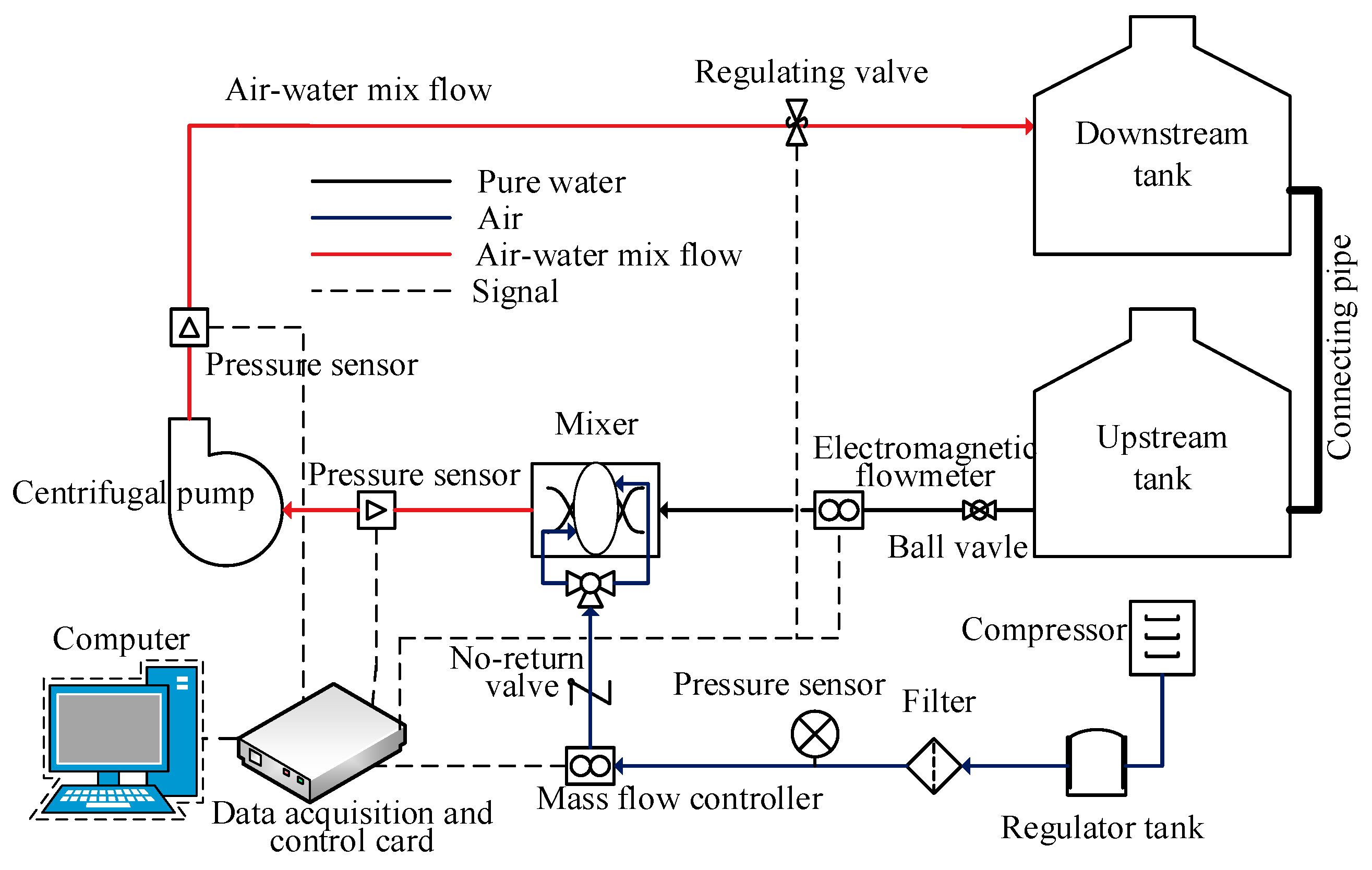
2.2. Experimental Test Rig

The pumps were measured on the open test rig designed for air entrainment shown in Figure 2. In this open type loop, the injection system of draughty air is driven at a constant 0.5 bar pressure by a compressor combined with a regulatory tank. The air mass flowrate is measured and well controlled by the Bürkert 8107 fluid control system (Bürkert Ltd, Huntersville, NC, USA) which can supply constant volume gas flow rate values under standard conditions (101,325 Pa, 25°). The initial air volume flow rate is calculated by measuring the pump inlet pressure to further calculate the α₀. Air-water mixed fluid is sucked into the pump flow passage and finally arrives at the downstream tank after going through the electric regulating valve. Air bubbles inside the mixed fluid exhaust to the atmosphere in the open type downstream tank, and the remaining pure water is consecutively run back into the loop. An electromagnetic flowmeter set between the upstream tank and the mixer is used to measure the volumetric flow rate of the pure water.

A LabVIEW acquisition program combined with a NI USB-6343 acquisition card (National Instruments Ltd, Austin, TX, USA) were used to obtain the signals, including the pressure, liquid flow rate, gas flow rate, rotational speed and torque values, collected by the sensors. Pump head and global efficiency is also obtained following ISO 9906: 2012 [28]. A dynamic pressure sensor is set located on the outlet pipe of the pump at twice the pipe diameter height distance. The biggest uncertainties of the measurement are a ±1.6% error of the pump head, ±3% error of the pump efficiency, ±1.7% error of the water flowrate, ±1% of the air void fraction and ±0.25% of the pressure pulsation, as calculated from the respective instrument precision.

As shown in Figure 3, the DAQ assistant provided by the LabVIEW software is used to configure the NI USB-6343-related channel, set the parameters of the sensors and related apparatus according to the measurement range of the instruments, input the collected signals into the host computer in real time, and finally output them for future data reduction. The various parameters such as head, efficiency and its dimensionless coefficient are defined as follows to reflect the performance changes of the centrifugal pump:

$$H=\frac{p_2-p_1}{\rho g}+\frac{v_2^2-v_1^2}{2g}+(z_2-z_1)$$

(1)

$$\eta =\frac{\rho gH{Q}_l}{P}$$

(2)

$$\alpha =\frac{Q_g}{Q_g+Q_l}$$

(3)

$$\rho =(1-\alpha ){\rho }_l+\alpha {\rho }_g$$

(4)

$$\phi =\frac{Q_l}{2\pi R_2{b}_2{u}_2}$$

(5)

$$\psi =\frac{gH}{u_2^2}$$

(6)

$$H_{th}=\frac{H}{\eta }$$

(7)

$${\psi }_{th}=\frac{g{H}_{th}}{u_2^2}\left(\frac{{\rho }_l}{{\rho }_g\times \alpha +{\rho }_l\times (1-\alpha )}\right)$$

(8)

2.3. Numerical Model and Setups

2.3.1. The Euler–Euler Inhomogeneous Multi-phase Flow Model

With the development of CFD technology, it has become a very helpful tool to analyze and study flow descriptions for modern scientific research and engineering practice, which provides us with more characteristics of the movement of the flow than experimental works.

Figure 4 shows the normal process for the gas-liquid two-phase flow calculation of centrifugal pumps, including 3D domain modeling, meshing, choosing turbulence model, setting boundary conditions, setting of the multiphase flow model, steady calculation, unsteady calculation, CFD post, etc.

The numerical calculation of the model pump flow field concerns the pump working under pure and air-water mixed flow conditions at different flow rates. The Reynolds average method is generally suitable for most flow dynamics problems in fluid machinery to solve the Navier-Stokes equation. Multiphase flow models are needed to start the two phase flow simulation, which are subdivided into homogeneous and inhomogeneous kinds. In the inhomogeneous model, both the velocity slip and the interphase mass and momentum transfer terms between the two phases are solved, regardless of the temperature field, for which the liquid phase is the continuous phase and the gas phase is a discrete one. Because the homogeneous model does not consider any velocity slips of different phases, this research adopts the inhomogeneous model to process the simulation. The selected particle model assumes a bubbly flow pattern for the mixed gas–liquid two-phase flow. In the following discussions gas–liquid here always refers to air-water. The continuity and the momentum equations are:

$$\frac{\partial }{\partial t}({\alpha }_k{\rho }_k)+\nabla \cdot ({\alpha }_k{\rho }_k{w}_k)=0$$

(9)

$$\frac{\partial }{\partial t}({\alpha }_k{\rho }_k{w}_k)+\nabla \cdot ({\alpha }_k{\rho }_k{w}_k\otimes w_k)=-{\alpha }_k\nabla p_k+\nabla \cdot ({\alpha }_k{\mu }_k(\nabla w_k+{(\nabla w_k)}^{\mathrm{T}}))+M_k+f_k$$

(10)

where k represents phase (l–liquid, g–gas), ρ_k represents density of the k phase (kg/m³), p_k represents pressure of k phase (Pa), α_k represents void fraction of k phase, μ_k represents dynamic viscosity of k phase (Pa·s), w_k represents relative velocity of the k phase fluid (m/s), M_k represents the phase interaction force of the k phase (N), f_k represents the added mass force related to the contribution of the impeller rotation (N). For the two-phase flow approach used in this study, the liquid phase is considered as the continuous phase using the RNG k-ε turbulence model. Meanwhile, the gas phase is considered as the discrete phase using the zero-equation theoretical model, which means only the so-called interfacial drag coefficients are considered between the liquid phase and gas phase [29]. It follows the relationships:

$$M_l=-M_g=\frac{3}{4}{c}_D\frac{{\rho }_l}{d_B}{\alpha }_g\left(w_g-w_l\right)\left|w_g-w_l\right|$$

(11)

with:

$$c_D=\{\begin{array}{ll}\frac{24}{R_e}(1+0.15R{e}^{0.687})& (R_e\le 1000)\\ 0.44& (R_e>1000)\end{array}$$

(12)

$$\mathrm{and}Re={\rho }_l\frac{\left|w_g-w_l\right|}{{\mu }_l}{d}_B$$

(13)

where d_B is the bubble diameter, c_D is the resistance coefficient.

2.3.2. Three-Dimensional Modelling for Calculation Domain

The flow domain of the pump was modeled in six parts using the commercial software Creo 3.0, taking pump 2 for example, as shown in Figure 5. It mainly divided into the inlet, the pump chamber, the wear ring, the impeller, the volute and the outlet parts. The inlet part was extended to ten times the pipe diameter, and the outlet part was extended by five times the pipe diameter, which avoids any possible backflow phenomena at the pump inlet and outlet.

2.3.3. Meshing and Irrelevance Verification

The three-dimensional water body is meshed by the ANSYS ICEM16.1 software. For better calculation convergence, hexahedral structured grid is adopted in the simulation process, the boundary layer mesh is added to the wall, and meshes in areas such as the volute tongue and inlet blade tip are partially encrypted. By using the hexahedral grid, the mesh quality is easy to flexibly control with boundary layer mesh guaranteeing. For the efficiency and accuracy of the calculation, the model pump is analyzed for grid independence at the design flow rate for both pumps. The design flow rate coefficient ϕ is 0.095 for pump 1 and 0.08 for pump 2. When the number of grids reaches about 2.78 for pump 1 and 3.25 million for pump 2, the change of two pump head coefficients basically remains stable, as shown in Figure 6.

Finally, the number of selected meshes is 2,775,915 and the number of mesh nodes is 2,945,000 for pump 1, the number of selected meshes is 3,255,253 and the number of mesh nodes is 2,886,504 for pump 2. The structured grid of the above calculation domain is shown in Figure 7. The dimensionless wall distance y + obtained by viscous grid spacing calculation is below 100 for all flow fields, which means the meshes used in this paper could satisfy the selected RNG k-ε turbulence model.

2.3.4. Boundary Conditions

In this study, the Euler-Euler heterogeneous flow model regardless of the influence of the temperature field is used. The liquid phase is defined as the continuous phase (ρ_l = 997.074 kg/m³) and the RNG k-ε homogeneous turbulence model is adopted. The gas phase is defined as the discrete phase (ρ_g = 1.185 kg/m³), using the zero-equation theory. The transfer way of the phase-to-phase uses the particle model and the rotational speed is set to 2900 r/min. At the entrance of the calculation domain, it is considered that the gas phase is uniformly distributed and we set that the two-phase inflow velocity is the same and it is uniform bubble flow, the gas phase is a spherical bubble which diameter is derived from the experimental one (0.2 mm), and the inlet gas volume fraction is respectively set to 1%, 3%, 5%, 7%, etc. The interface between impeller and volute is set to frozen rotor for steady calculation, and the transient rotor stator for the unsteady calculation. The steady calculation result is used as the initial condition for the unsteady calculation.

In general, the final accuracy of an unsteady simulation is a function of the time step. It would significantly increase the calculation time if we set a small time step. Courant number defined by Equation (14) is always used as criterion to judge if the time step satisfies the periodic numerical simulation [30]:

$$C_o=v\frac{\Delta t}{L}<100$$

(14)

where L is the smallest size of the grid, v is the main flow velocity and Δt is the time step. The maximum v is below 30 m/s, and L is more than 0.1 mm according to the pump geometry and grid information. The simulation set the time step as 1.7248 × 10⁻⁴ s and the total time as 0.2069 s. Then, the calculated maximum C_o is 51.744, which satisfies the time step independence.

The boundary condition at inlet is set according to the actual measured pressure and selected volume flowrate of air. The turbulence intensity is set to the medium turbulence density (5%). The boundary condition at outlet is set as mass flow. For wall boundary conditions, the gas boundary adopts a free-slip wall surface.

3. Experimental Analysis on Pump Handing Ability of Gas Entraining

Each performance test is carried out from a low water flow rate to large water flow rate maintaining a constant α₀. Then, similar procedures are used to obtain the overall pump performance curves under different α₀ by increasing the volume of entrained air. In order to evaluate the pump handing ability of gas entrainment regardless of rotational speed, all performance parameters are dimensionless.

3.1. Overall Pump Performance at Single Water Conditions

Figure 8 and Figure 9 respectively show the overall pump performances for head coefficient (Figure 8a,b) and global efficiency (Figure 9a,b) versus flow coefficient. The pump 2 head coefficient is slightly higher than that of pump 1 with less influence of the rotational speed, probably due to higher Reynolds number value based on a higher outlet impeller diameter. Pump 2 is more sensitive to cavitation problems for high rotational speeds and flow rates. This is the reason why the performance curves in Figure 8b drop when the flow coefficient is bigger than 0.1, so in terms of single and two-phase flow performance comparisons, results obtained for rotational speeds lower than 1800 r/min and flow coefficient below 0.1 can be used. A comparison between head and theoretical head coefficients are given in Figure 10, respectively, for the same rotational speed values. Theoretical head coefficient is defined as the ratio of the measured head divided by the measured efficiency. This is the reason why its value tends to infinity when the flow coefficient close to zero as shown in Figure 10b using measurement results. The straight line corresponds to the ideal curve obtained from the so-called Euler equation assuming steady conditions without inlet flow swirl and constant mean relative outlet angle at the impeller exit.

This curve starts from ψ_th = 1 for a flow coefficient equal to zero. It fits quite well with the experimental one for flow coefficients higher than 0.065, which value corresponds to 70% of the pump design conditions. The two pumps have similar head coefficient curves and theoretical head coefficient curves at 1450 r/min.

3.2. Overall Pump Performance at Gas-Liquid Two-Phase Flow Conditions

3.2.1. Evolution of Water Flow Rate and Head Coefficient with Increased α₀

Figure 11 show the performance maps for the pumps’ rated rotational speeds. Under non- cavitation conditions, pump 2 is able to pump a high inlet void fraction for a wider range of flow coefficients with better head coefficients. This can be easily seen for inlet void fractions up to 10% for example. The corresponding theoretical head coefficient curves are presented in Figure 12. For pump 2, a unique curve is obtained for all inlet void fraction values up to 10%. This is not the case for pump 1, for which only a single curve is obtained in the inlet void fraction range from 0% to 8%. The ideal theoretical head coefficient curve, corresponding to the straight line, is exactly the same one for both pumps. This means that the both impellers deliver the same mean relative outlet flow angle for flow coefficients higher than 70% of the nominal one for a maximum α₀ of 8%.

3.2.2. Evolutions of Theoretical Pump Degradation for Two Different Flow Rates

Two-phase head coefficient ratio ψ*_tp is often used to characterize pump degradation level, as is defined by Equation (15). ψ_tp is the actual head coefficient under two-phase flow condition, ψ₀ is the head coefficient obtained only for liquid. The corresponding curves are given in Figure 8 for the two pumps at the rated rotational speed and three different flow coefficients. For the pump 2 case, it can be observed that the more the flow coefficient decreases, the better the head coefficient ratio stays at a high level before pump breakdown. Both pumps exhibit quite close two-phase performance curve degradation levels for flow coefficient value φ = 0.065 (see Figure 13e,f); however, the performance of pump 1 suddenly drops for α₀ = 8–9%, whereas pump 2 is still working for α₀ = 10%.

$${\psi }_{tp}^{*}=\frac{{\psi }_{tp}}{{\psi }_0}$$

(15)

When the flow coefficient decreases, pump 2 always has a better performance ratio compared with pump 1, for an equivalent rotational speed. This could be related to the difference of the impeller radius ratio R₂/R₁ and the incidence angle variation of both pumps, which are different. Further analysis should be conducted on these parameters.

Whatever pump is considered, a clear effect of the rotational speed exists for pump two-phase flow performances as already shown by several authors. Since both pumps have different outlet impeller radii, it is interesting to compare the performance ratio for the same rotational velocity at impeller outlet u₂. To do so, a comparison between pump 1 for 1800 r/min and pump 2 for 1450 r/min for φ = 0.065 could be done. Both curves look the same up to α₀ = 5%. Pump 1 still pumps two phase mixtures up to 7% before breakdown, so one can conclude that the performance degradation is quite the same when the impeller outlet rotational speed u₂ is the same, but the bigger rotational speed allows one to extend the pump’s ability to work for higher inlet void fractions. This is probably partly related to the fact that inlet bubbles are more easily broken at the pump inlet when the rotational speed is bigger.

4. Flow Pattern Analysis Inside the Pump Passage

4.1. Numerical Pump Performance and the Experimental Verification

Figure 14 shows the comparison of pump head coefficient curves and pump efficiency curves at different α₀ between the experiment and the simulation for the two model pumps under a design rotational speed of 2900 r/min.

For pump 2, cavitation occurs at high flow rates. However, CFD results are not performed for these conditions, so only results without cavitation flow are shown for pump 2 in order to avoid the interference of cavitation bubbles. As seen from the figures, the test results and the simulation results maintain a good consistent trend for both head coefficients and efficiency for all selected α₀ values.

For pure water conditions, the differences between the experiments and simulation for both pumps are slightly bigger under larger flowrate than that under a low flowrate. The maximum residual of the head is 5.9% and of the efficiency is 1.8% for pump 1, the maximum residual of the head is 4.3% and of the efficiency is 2.0% for pump 2, which are within the allowable deviation range and can meet the requirements of subsequent analysis. For two phase flow conditions, the simulation value is in good agreement with the experimental value, except at a low flowrate for pump 1, which is more sensitive to bubbly motion. The simulation value of small flow rate and large flow rate of pump 2 is in poor agreement with the experimental value after α₀ reaches 7%, but the trend is the same with the flow rate. The zone with high efficiency of pump 2 is narrower than that of pump 1. The calculation results are still reliable up to α₀ equal to 3% and rather qualitatively acceptable when α₀ reaches 7%, indicating that the selected Euler-Euler inhomogeneous two-phase flow model is suitable for the simulation of internal flow of such centrifugal pumps up to α₀ equal to 7%.

4.2. Flow Inside the Impeller and Volute Section

Figure 15 shows the air phase distribution inside the impeller passage of different α₀ values under the design conditions for two pumps. The relative location of the volute tongue in Figure 15, Figure 16, Figure 17 and Figure 18 is the same. When α₀ increases, the local air content inside the impeller passage gradually increases. The air is mainly distributed on the blade suction side and the outlet part of the impeller flow passage. Then, air gradually moves toward the outlet of the impeller flow passage along the blade suction side. It can also be observed from the figures that when α₀ reaches 5%, the air-water separation phenomenon begins to occur at the outlet of the impeller flow passage. In particular when α₀ is 7%, the air-water separation phenomenon is more obvious, but the air-water coexistence is dominant.

The flow field distributions of pump 1 and pump 2 are similar, and some results of pump 1 have been reported before [15,16]. Moreover, pump 2 already shows better handing ability for air entrainment, so the follow-up analysis is mainly based on the flow field information of pump 2 then. Turbulent kinetic energy is a physical quantity (k) commonly used in fluid mechanics to express the degree of turbulent pulsation. The turbulent intensity is often used to estimate the turbulent kinetic energy. The general Equation (16) is used to calculate the turbulent kinetic energy. It is a physical quantity commonly used to describe the loss of the viscosity of the fluid and the extent of the pulsation diffusion:

$${\mathrm{T}}_{\mathrm{KE}}=\frac{3}{2}{\left(ul\right)}^2$$

(16)

where u represents the average velocity (m/s), l represents the turbulence intensity.

Figure 16 shows the turbulent kinetic energy distribution in the impeller passage for four different α₀ values under design conditions. It can be observed from the figures that as the α₀ increases, the turbulent kinetic energy in the impeller increases gradually, and the distribution in the flow-path of the impeller is uniform. When the inflow α₀ is 7%, the turbulent kinetic energy increases significantly at the impeller outlet and dissipation is more serious.

Figure 17 shows the turbulent kinetic energy distribution when the α₀ is 3% under different four flowrates. As seen from the figures, when the α₀ is 3%, the turbulent kinetic energy is distributed evenly in each impeller flow-path, and it is the smallest under the design flow conditions. The turbulent kinetic energy is larger under the small flow condition than the large flow condition. The high asymmetrical intensity in Figure 17a means the distribution of turbulent kinetic energy under two phase flow is also related to the flow rate, which corresponds to the change on the slope curve of the theoretical head coefficient. The smaller the flow rate, the higher the kinetic energy, and the more uneven the distribution. It rotates relative to the impeller because of the rotor-stator interaction, which is similarly referred in the literature [15].

Comparing with the distribution of the air phase in Figure 15, it can be seen that the distribution of the turbulent kinetic energy is closely related to the distribution of the air inside the impeller, that is, the more the air void fraction, the greater the turbulent kinetic energy in this region, indicating that the air accumulation causes the increase of the turbulence level in the flow passage and the loss of the fluid viscous dissipation, which affects the exchange and transfer of fluid energy inside the impeller channel, resulting in the falling of the model pump performance.

Figure 18 shows the distribution of the air phase on the iso-surface when the air content is 20% in the impeller under the rated flow rate. It can be seen that under the same α₀, the lower the air phase iso-surface, the more the air, and the simulation results show that the iso-surface is almost non-existent when the air phase is 100%, indicating that the air and the liquid are not completely separated in the flow path but exist in an air-water mixed state when the inflow air content is within 7%. When the α₀ reaches 7%, the bubbles occupy about 40% of the impeller flow-path. Compared with the centrifugal pump previously studied by the same research group, this centrifugal pump has a stronger ability to transport air and liquid. Therefore, it is possible to deliver the liquid with higher α₀. The air enters the volute flow-path from the impeller flow-path and finally flows to the outlet pipe. The bubbles with high air content gradually move toward the impeller outlet along the blade suction side.

Inside the volute channel, the air with high air content is mainly distributed far from the impeller. Around the tongue area, the air with high air content is mainly distributed away from the tongue and finally flows to the outlet pipe, which is consistent with the flow pattern distribution observed in the literature [5].

Figure 19 shows the location of eight volute sections. Figure 20 and Figure 21 present the air phase distribution and the velocity streamline of air phase inside the volute passage for different α₀. As observed from the figures, the air void on the front shroud side of each section of the volute flow passage is more than that on the hub side, and as α₀ increases, the local air void in the volute increases gradually, which causes the velocity streamline to change and makes it easy to generate vortices. The generation of vortices further aggravates the air stagnation region in this part, resulting in a large air accumulation. Moreover, this will increase the vortex intensity and the loss, which results in the falling of the pump performance. It shows that the air accumulation in the volute flow-path is closely related to the generation of vortices and deteriorate pump performance, which also affect the pump handing ability to sustain two phase flow.

4.3. Numerical Unsteady Pressure Results

4.3.1. Monitoring Point Position

In order to obtain the pressure pulsation characteristic of each section inside the volute, twelve monitoring points are set as follows: the monitoring point P1 is set at the intersection of Section 1 and the middle streamline of the volute flow passage; the monitoring point P3 is set at the intersection of Section 3 and the middle streamline of the volute flow passage, and so on. By the way, P5b, P5 and P5d are the points on the V section of the volute, located at the back, middle and bottom of the volute respectively. Pgs1–4 locate near the tongue on the IX section of the volute. Po is set at the outlet part of the pump with the same location with the experimental dynamic pressure sensor. The locations of the monitoring points are shown in Figure 22.

4.3.2. Experimental Unsteady Pressure Validation

During this measurement, the sampling frequency is set to 5000 Hz, and the sampling time is set to 30 s. After the pump is running stably at a constant α₀ of flowrate from zero to pump break up, the data acquisition system collects the unsteady pressure automatically when it starts the acquisition program. In this test, each working condition is measured 10 times, and the RMS averaging mode is applied to the 10th measured raw data, and the Hanning window function is used to reduce the measurement inaccuracy caused by the leakage. Since the outlet part of the pump has more influence on system reliability for bigger absolute pressure than that at the inlet part, the pressure fluctuation information at the monitoring point Po is used to verify the simulation results in this study. In order to present it in a normalized form, a non-dimensional pressure coefficient C_P expressed as follows is introduced:

$$C_P=\frac{\left(p-\overline{p}\right)}{0.5\rho u_2{}^2}$$

(17)

where p represents the static pressure (Pa), $\overline{p}$ represents the average of the static pressure (Pa), ρ represents the density of the air-water mixed fluid (kg/m³), u₂ represents the circumferential velocity at blade outlet (m/s). The pressure pulsation is further analyzed by using the fast Fourier transform (FFT) method under Q_d at different α₀ values from 0 to 7%.

Figure 23 shows the spectrum results of Po under different flow conditions for both experiment and simulation. C_P^* presents the amplitude at each frequency. f_n is the impeller passing frequency. It can be observed from the figures that the main frequency of the pressure pulsation is the blade frequency under pure water conditions and even under working conditions where α₀ is below 5% from both the experiment and simulation results. The amplitude value at the blade passing frequency decreases at α₀ equal to 1%, which indicates that a small amount of air entrainment is actually beneficial to the flow stability. The appearance of the peak at low frequency increases gradually with the increase of α₀. Three times the axial passing frequency is dominant when the α₀ is 5%. The results of the numerical simulation present the same trend as those of the experiment, except for a few low frequency characteristics when α₀ increases. Physically, the mixture with air will gradually block some of the flow passage of the impeller when the centrifugal pump delivers an air-water mixture flow, resulting in a reduction of the water flowrate through the blade channel, which will reduce the local pressure in the flow path. This will exacerbate the accumulation of air. As a result, the instability of the pressure pulsation increases, and the fluctuation of pressure pulsation will be more obvious. At the design flow point, the initial development of internal cavitation caused by the test system causes the pressure pulsation to fluctuate greatly under pure water conditions and has a large amplitude. When the inflow content is 5%, it is found that the main frequency of pressure pulsation is at 1/2 the blade frequency, and more broadband signal bands are generated nearby. Combined with the changes in the pump performance curve from experiments at this condition, it is explained that cavitation has an important influence on external performance characteristic and dynamic characteristics of the centrifugal pump.

Figure 24 shows the root-mean-square (RMS) value of the pressure pulsation obtained by performing related processing for both experiment and simulation results at Po.

As seen from the figures, the RMS value gradually decreases as the flow rate increases, reflecting the change of the pressure pulsation amplitude during the measured time period, indicating that the pressure fluctuation is greater under small flow conditions, which is due to the unstable flow under these conditions. Therefore, the internal flow conditions can be reflected by the RMS, which provides a theoretical basis for the monitoring and diagnosis of the pump. Under the same flow condition, with the increase of the α₀, the RMS increases first and then decreases. At the same α₀, the RMS of the design flow point is minimal. The greater the deviation from the design condition point, the more the value. This is due to the instability of the flow under the small flow, this is easy to produce reflux, resulting in a large fluctuation of pressure pulsation at this time.

4.3.3. Numerical Pressure Pulsation Analysis Inside the Volute Passage of Pump 2

Figure 25 show the time domain diagram of the pressure for some selected monitoring points under Q_d when air is entrained. As seen from it, the pressure of the impeller will have six “peak-valley” regular fluctuations in one rotation cycle, which is consistent with the number of model pump blades in this study. The periodicity of the pressure fluctuation with α₀ is 3% became worse than the case when α₀ is 1%. The pressure fluctuation of the monitoring points near the tongue is more intense than the monitoring points away from the tongue, indicating that the flow instability in the vicinity of the tongue is strong. As can be seen by the comparison between Figure 25c,d, the pressure fluctuation of monitoring point Pgs1 is less intense than at Pgs2, that is, the pressure fluctuation on the side of the tongue near the impeller is smaller than the side of the tongue in the volute, which may be related to the accumulation of air in this position.

Frequency spectrum diagrams of pressure the pulsation at four different α values for different monitoring points are presented in Figure 26, Figure 27 and Figure 28. As seen from the figures, the amplitude of each monitoring point is mainly concentrated in the blade frequency and its double frequency. When the α₀ values are 1% and 3%, the main frequency of the pressure pulsation is the blade passing frequency. The generation and range of broadband pulsation will gradually increase in the low frequency region when the α₀ increases. However, when the α₀ reaches 5%, the amplitude of the pressure pulsation shaft frequency occupies the main part, which is almost consistent with the results of the pressure pulsation test in this paper.

Figure 28 is the pressure pulsation dominant frequency of the V section of the volute. The amplitude of the pressure pulsation main frequency is greatly affected by the α₀. The basic law is similar to other monitoring points, but because this position is the farthest from the volute tongue area and the rotor-stator interaction influence is weakest, leading to the amplitude of the pressure pulsation main frequency of is the smallest. However, probably because the air is easy to gather here seen form pre-analysis, the characteristics of low-frequency pulsation in this area are the most obvious.

5. Conclusions

Based on experimental investigations, overall performance comparisons between two different centrifugal pump designs have been presented under two-phase flow conditions for different inlet void fractions and rotational speeds. A full 3D-URANS simulation using the Euler–Euler inhomogeneous two-phase flow model was carried out to determine the flow characteristics. The following main conclusions are obtained through analyzing the experimental and numerical results of the selected model pumps:

(1)

Pump 2 is less sensitive to gas-liquid two-phase flow than pump 1. For the rated rotational speed of 2900 r/min, pump 2 still able to deliver two-phase mixtures up to 10% before pump shut-off, whereas pump 1 is limited to 8%. The performance degradation of both pumps is quite the same for equivalent impeller outlet rotational speed, but a greater rotational speed allows one to extend the pump’s ability to work for higher inlet air void fractions. For a given angular rotational speed, a greater impeller outlet radius allows one to extend the pump’s ability to work at higher inlet void fractions.

(2)

The pump performance obtained by simulation under inlet air void fractions below 7% are consistent with the experimental ones, indicating that the selected Euler-Euler heterogeneous flow model can satisfy the calculation needs under low inlet air void fraction conditions. The degradation slope of the simulation curves increases more when the inlet void fraction increases, with a negative signof the decreasing head and efficiency.

(3)

The generation of vortices intensifies the accumulation of air, and then affects the energy exchange and transfer of the rotating impeller, resulting in the degradation of pump performance. Bubbles always gather on the suction side of the blade surface at first, and gradually gather in the entire flow passage with the increase of inlet air void fraction. Some bubbles flow exiting from the impeller outlet move to the volute, gather along the wall surface and finally are forced to the outlet pipe. The phenomenon of air-water separation begins when the inlet air content is 5%.

(4)

Pressure pulsation is mainly caused by rotor-stator interaction between impeller and volutes and vortices in the whole flow passage. The addition of air fraction in the flow-path leads to intensify the degree of vortices. The time domain diagram of pressure for the monitoring points under different α₀ presents six “peak-valley” periodic variation rules consistent with the number of blades, and the pulsation pressure fluctuation near the volute tongue is greater than that far away from the tongue. The pressure pulsation amplitude at low frequency area gradually increases with the increase of α₀ and produces broadband pulsation. Its range gradually widens with the increase of α₀. When α₀ reaches to 5%, the pressure pulsation amplitude at shaft passing frequency account for the main part, which is consistent with the test results.

References

1. Val, S.L.; Robert, R.R. Centrifugal Pumps: Design and Application, 2nd ed.; Gulf Professional Publishing: Houston, TX, USA, 2013. [Google Scholar]
2. Jiang, Q.; Heng, Y.G.; Liu, X.B.; Zhang, W.B.; Bois, G.; Si, Q.R. A review of design considerations of centrifugal pump capability for handling inlet gas-liquid two-phase flows. Energies 2019, 12, 1078. [Google Scholar] [CrossRef] [Green Version]
3. Noghrehkar, G.R.; Kawaji, M.; Chan, A.M.C.; Nakamura, H.; Kukita, Y. Investigation of centrifugal pump performance under two-phase flow conditions. J. Fluids Eng. 1995, 117, 129–137. [Google Scholar] [CrossRef]
4. Stel, H.; Ofuchi, E.; Sabino, R.; Ancajima, F.; Bertoldi, D.; Marcelino, N.; Morales, R. Investigation of the motion of bubbles in a centrifugal pump impeller. J. Fluids Eng. 2019, 141, 031203. [Google Scholar] [CrossRef]
5. Si, Q.R.; Zhang, H.Y.; Bois, G.; Zhang, J.F.; Cui, Q.L.; Yuan, S.Q. Experimental investigations on the inner flow behavior of centrifugal pumps under inlet air-water two-phase conditions. Energies 2019, 12, 4377. [Google Scholar] [CrossRef] [Green Version]
6. Murakami, M.; Minemura, K. Effects of entrained air on the performance of a centrifugal pump: 1st report performance and flow conditions. Bull. JSME 1974, 17, 1047–1055. [Google Scholar] [CrossRef]
7. Murakami, M.; Minemura, K. Effects of entrained air on the performance of a centrifugal pump: 2nd report effects of number of blades. Bull. JSME 1974, 17, 1286–1295. [Google Scholar] [CrossRef] [Green Version]
8. Furukawa, A.; Shirasu, S.-I.; Sato, S. Experiments on air-water two-phase flow pump impeller with rotating-stationary cascades and recirculating flow holes. JSME Int. J. Ser. B 1996, 39, 575–582. [Google Scholar] [CrossRef] [Green Version]
9. Furukawa, A.; Ohshita, S.; Okuma, K.; Watanabe, S. Development of air/water two-phase flow centrifugal pump and its operating characteristics. In Proceedings of the 4th ASME-JSME Joint Fluids Engineering Conference, Honolulu, HI, USA, 6–10 July 2003. [Google Scholar]
10. Cappellino, C.A.; Roll, D.R.; Wilson, G. Design considerations and application guidelines for pumping liquids with entrained gas using open impeller centrifugal pumps. In Proceedings of the 9th International Pumps User Symposium, College Station, TX, USA, 3–5 March 1992; Volume 1169, pp. 51–60. [Google Scholar]
11. Mansour, M.; Wunderlich, B.; Thévenin, D. Experimental study of two-phase air/water flow in a centrifugal pump working with a closed or semi-open impeller. In Proceedings of the ASME Turbo Expo 2018: Turbomachinery Technical Conference and Exposition, Oslo, Norway, 11–15 June 2018. [Google Scholar]
12. Li, X.J.; Chen, B.; Luo, X.W.; Zhu, Z.C. Effects of flow pattern on hydraulic performance and energy conversion characterisation in a centrifugal pump. Renew. Energy 2019. [Google Scholar] [CrossRef]
13. Kosyna, G.; Suryawijaya, P.; Froedrichs, J. Improved understanding of two-phase flow phenomena based on unsteady blade pressure measurements. J. Comput. Appl. Mech. 2001, 2, 45–52. [Google Scholar]
14. Schäfer, T.; Bieberle, A.; Neumann, M.; Hampel, U. Application of gamma-ray computed tomography for the analysis of gas holdup distributions in centrifugal pumps. Flow Meas. Instrum. 2015, 46, 262–267. [Google Scholar] [CrossRef]
15. Si, Q.R.; Cui, Q.L.; Zhang, K.Y.; Yuan, J.P.; Bois, G. Investigation on centrifugal pump performance degradation under air-water inlet two-phase flow conditions. La Houille Blanche 2018, 3, 41–48. [Google Scholar] [CrossRef] [Green Version]
16. Si, Q.R.; He, W.T.; Bois, G.; Cui, Q.L.; Yuan, S.Q.; Zhang, K.Y. Experimental and numerical studies on inner flow characteristics of centrifugal pump under air-water inflow. Int. J. Fluid Mach. Syst. 2019, 12, 31–38. [Google Scholar]
17. Shao, C.L.; Li, C.Q.; Zhou, J.F. Experimental investigation of flow patterns and external performance of a centrifugal pump that transports gas-liquid two-phase mixtures. Int. J. Heat Fluid Flow 2018, 71, 460–469. [Google Scholar] [CrossRef]
18. Furuya, O. Analytical model for prediction of two-phase (noncondensable) flow pump performance. J. Fluids Eng. 1985, 107, 139–147. [Google Scholar] [CrossRef]
19. Minemura, K.; Uchiyama, T. Prediction of pump performance under air-water two-phase flow based on a bubbly flow model. J. Fluids Eng. 1993, 115, 781. [Google Scholar] [CrossRef]
20. Minemura, K.; Uchiyama, T.; Shoda, S.; Egashira, K. Prediction of air-water two-phase flow performance of a centrifugal pump based on one-dimensional two-fluid model. J. Fluids Eng. 1998, 120, 237–334. [Google Scholar] [CrossRef]
21. Zhu, J.J.; Zhang, H.Q. A review of experiments and modeling of gas-liquid flow in electrical submersible pumps. Energies 2018, 11, 180. [Google Scholar] [CrossRef] [Green Version]
22. Minemura, K.; Uchiyama, T. Three-dimensional calculation of air-water two-phase flow in centrifugal pump impeller based on a bubbly flow model with fixed cavity. JSME Int. J. Ser. B Fluids Therm. Eng. 1993, 37, 726–735. [Google Scholar] [CrossRef] [Green Version]
23. Clarke, A.P.; Issa, R.I. Numerical prediction of bubble flow in a centrifugal pump. Multiphase Flow 1995, 133, 175–181. [Google Scholar]
24. Caridad, J.; Kenyery, F. CFD analysis of electric submersible pumps (ESP) handling two-phase mixtures. J. Energy Resour. Technol. 2004, 126, 99–104. [Google Scholar] [CrossRef]
25. Müller, T.; Limbach, P.; Skoda, R. Numerical 3D RANS simulation of gas-liquid flow in a centrifugal pump with an Euler-Euler two-phase model and a dispersed phase distribution. In Proceedings of the 11th European Conference on Turbomachinery, Fuild Dynamics and Thermodynamics, Madrid, Spain, 23–25 March 2015. [Google Scholar]
26. Zhu, J.J.; Zhang, H.Q. Numerical study on electrical-submersible-pump two-phase performance and bubble-size modeling. SPE Prod. Oper. 2017, 32, 267–278. [Google Scholar] [CrossRef]
27. Si, Q.; Bois, G.; Jiang, Q.; He, W.; Asad, A.; Yuan, S. Investigation on the handling ability of centrifugal pump under air-water two-phase inflow: Model and experimental validation. Energies 2018, 11, 3048. [Google Scholar] [CrossRef] [Green Version]
28. ISO 9906: 2012. Rotodynamic Pumps-Hydraulic Performance Acceptance Tests-Grades 1, 2 and 3. Available online: https://www.iso.org/standard/41202.html (accessed on 31 May 2012).
29. Clift, R.; Grace, J.R.; Weber, M.E. Bubbles, Drops and Particles; Academic Press: New York, NY, USA, 1978. [Google Scholar]
30. Wang, C.; Hu, B.; Zhu, Y.; Wang, X.L.; Luo, C.; Cheng, L. Numerical study on the gas-water two-phase flow in the self-priming process of self-priming centrifugal pump. Processes 2019, 7, 330. [Google Scholar] [CrossRef] [Green Version]
Figure 1. Meridional shapes of pump 1 and pump 2 (all numbers with unit of mm).
Energies 13 00065 g001
Figure 2. Schematic diagram of the gas entrainment two-phase flow test system for centrifugal pumps.
Energies 13 00065 g002
Figure 3. The signal acquisition process.
Energies 13 00065 g003
Figure 4. Calculation process.
Energies 13 00065 g004
Figure 5. Three-dimension modeling of the model pump 2 domain.
Energies 13 00065 g005
Figure 6. Grid independence check for the two pump domains.
Energies 13 00065 g006
Figure 7. Structure meshes of the model pumps: (a) Pump 1; (b) Pump 2.
Energies 13 00065 g007
Figure 8. Pump head coefficients with pure water: (a) Pump 1; (b) Pump 2.
Energies 13 00065 g008
Figure 9. Global efficiency of the pump with pure water: (a) Pump 1; (b) Pump 2.
Energies 13 00065 g009
Figure 10. Comparison with pure water: (a) Head coefficient; (b) Theoretical head coefficient.
Energies 13 00065 g010
Figure 11. Head coefficient at different inlet air void fractions: (a) pump 1; (b) pump 2.
Energies 13 00065 g011
Figure 12. Theoretical head coefficient at different inlet air void fractions: (a) pump 1; (b) pump 2.
Energies 13 00065 g012
Figure 13. Two-phase head coefficient ratio at different rotational speed: (a) Pump 1 φ = 0.04; (b) Pump 2 φ = 0.04; (c) Pump 1 φ = 0.058; (d) Pump 2 φ = 0.058; (e) Pump 1 φ = 0.065; (f) Pump 2 φ = 0.065.
Energies 13 00065 g013aEnergies 13 00065 g013b
Figure 14. Comparison between experimental and simulated results: (a) Pump1 head coefficient; (b) Pump1 efficiency; (c) Pump2 head coefficient; (d) Pump2 efficiency.
Energies 13 00065 g014
Figure 15. Gas phase distribution in impeller at different α0: (a) pump1, α0 = 1%; (b) pump1, α0 = 5%; (c) pump1, α0 = 7%; (d) pump2, α0 = 1%; (e) pump2, α0 = 5%; (f) α0 = 7%.
Energies 13 00065 g015
Figure 16. Turbulent kinetic energy distribution in impeller of pump 2 at different α0: (a) 1%; (b) 3%; (c) 5%; (d) 7%.
Energies 13 00065 g016
Figure 17. Turbulent kinetic energy distribution in impeller of pump 2 at α0 = 3%: (a) 0.6Qd; (b) 0.8Qd; (c) Qd; (d) 1.2Qd.
Energies 13 00065 g017
Figure 18. Contour map of 20% air equivalent surface in the impeller and volute of pump 2 at different α0: (a) 1%; (b) 3%; (c) 5%; (d) 7%.
Energies 13 00065 g018
Figure 19. Location of eight volute sections for pump 2.
Energies 13 00065 g019
Figure 20. Air phase distribution at different volute sections of pump 2 at different α0: (a) 1%; (b) 3%; (c) 5%; (d) 7%.
Energies 13 00065 g020aEnergies 13 00065 g020b
Figure 21. Air-phase velocity streamline at different sections of volute of pump 2 with different α0: (a) 1%; (b) 3%; (c) 5%; (d) 7%.
Energies 13 00065 g021
Figure 22. Location of the monitoring points for pump 2.
Energies 13 00065 g022
Figure 23. Frequency domain diagram of the pressure pulsation at the outlet section of pump 2 for different α0 under Qd: (a) Experiment; (b) Simulation.
Energies 13 00065 g023
Figure 24. RMS of pressure pulsation at the outlet section of pump 2 for different α0 under Qd: (a) Experiment; (b) Simulation.
Energies 13 00065 g024
Figure 25. Time domain diagram of the pressure for pump 2 at different α0: (a) P1~P8, 1%; (b) P1~P8, 3% (c) Pgs1~Pgs4, 1%; (d) gs1~Pgs4, 3%.
Energies 13 00065 g025aEnergies 13 00065 g025b
Figure 26. Frequency domain diagram of pressure for pump 2 at different α0 along volute flow passage: (a) 1%; (b) 3%; (c) 5%; (d) 7%.
Energies 13 00065 g026
Figure 27. Frequency domain diagram of pressure for pump 2 at different α0 near volute tongue: (a) 1%; (b) 3%; (c) 5%; (d) 7%.
Energies 13 00065 g027
Figure 28. Frequency domain diagram of pressure for pump 2 at different α0 near section V: (a) 1%; (b) 3%; (c) 5%; (d) 7%.
Energies 13 00065 g028aEnergies 13 00065 g028b