Design and Experiment of a Power Sharing Control Circuit for Parallel Fuel Cell Modules

Abstract

In this paper, a novel control circuit that can connect fuel cell (FC) modules in parallel is proposed, which is particularly useful when the employed FCs have different electrical characteristics. Conventional methods (e.g., DC/DC converters) are not applicable in such situations because they cannot regulate the power output of each source in a parallel-connected topology. Consequently, the uniformity requirement of FCs increases and becomes costly. In contrast to existing methods, the proposed method adopts a novel power-feedback method to control the power output of each FC module under both rated conditions and load changes, which in turn determines the operating point of each FC module. Therefore, the uniformity requirement can be relaxed. For proof of concept, the experiments employed two FC-like sources with different I–V characteristics. The experimental results indicated that the power assignment under the rated condition had a relative error of < 6.62%. The distribution ratio error under the load change was < 7.43%. Therefore, the proposed method can regulate the power output (operation point) of each parallel-connected FC-like power source.

1. Introduction

Fuel cells (FCs) have been a focus of power generation system research because of their environmentally friendly qualities and high energy-conversion efficiency [1]. In an FC system, the output power of an FC module is approximately 3–10 kW. FC modules must be aggregated to yield the necessary power to build a power generation system with megawatt capacity. Because of the manufacturing process variance and aging issues [2], all FC modules cannot yield the same performance. Aggregating power units of different characteristics together without any regulation measures may lead to issues such as uneven power output of each unit, reliability, and thermal runaways [3,4]. Therefore, FC modules are often aggregated with the assistance of power electronics [5,6,7].

An FC produces electricity through electrochemical reactions. Unlike conventional voltage or current sources, the output voltage of an FC varies greatly with its output current [8]. Figure 1a shows that the output voltage of an FC decreases as the output current increases. On the other hand, the corresponding output power may either increase or decrease as the output current increases, depending on the output current. Figure 1b shows that the electrochemical reactions of the FC would produce electricity and heat and the corresponding energy-conversion efficiency varies with the output current. Therefore, each operation point of an FC represents not only different power outputs but also different energy-conversion efficiency, hydrogen utilization, operating temperature, and heat output [9,10,11]. For instance, a typical design would have the FC work at point C in Figure 1a [11]. Working to the right of point D would lead to excessive use of hydrogen. By contrast, operating near point B would considerably reduce the energy-conversion efficiency. Therefore, in a parallel-connected FC module system, if the aforementioned power electronics cannot control the power output of each FC module, the FC is likely to function at an undesirable operation point, which could lead to either low electrical energy efficiency or permanent damage. The conventional power electronics for FC systems, such as direct current (DC) link, high-frequency alternating current (AC) link, and multilevel architectures [12], may be inadequate because they cannot control the power sharing. Consequently, the FC module needs to have a strict uniformity requirement to secure an operation window. This uniformity is associated with cost-intensive processes, such as module channel design, flow control, and thermal management [13].

Droop converters implement the output voltage as a function of the output current [14,15,16]. This has led the droop converter to be the most used power electronic device for achieving power sharing in a parallel-operated power system. However, conventional droop methods have poor load voltage regulation capability [17]. Therefore, many researchers have proposed combining the droop method and DC/DC converter technique to achieve both power sharing and load voltage regulation. These methods are now crucial to the DC microgrid technology [17,18,19]. Baritor et al. [17] proposed using the duty ratio of a DC/DC converter to realize a virtual resistance for the droop method. The advantage is that the control actions depend on local variables alone. Anand et al. [18] proposed a control method that uses the local current, average current in a network, and load voltage to determine the duty ratio of the DC/DC converter. One possible drawback is that the controller requires information from other devices in the network, albeit only low-speed communication. Although the aforementioned approaches have claimed power-sharing capability, they are in fact current-sharing methods because they are all developed from the droop method.

The new technologies, such as DC microgrid methods, cannot be directly applied to FCs because an FC is not a constant-voltage source [20,21]. Therefore, current sharing in FCs is not equivalent to power sharing. A few researchers have proposed new power electronics exclusively for connecting FCs in parallel. Choe et al. [20] proposed a master–slave controller with power-sharing capability for FCs. Both the master and slave controllers are similar to conventional current-feedback DC/DC converters, except they employ additional digital controllers to obtain the power information. Furthermore, the slave controller obtains its reference current command by scaling the reference power command provided by the master controller. Grover et al. [21] focused on the fuel starvation problem in FCs and proposed another master–slave controller to equally distribute the load current to parallel-operated FCs. The master controller controls the load voltage, whereas the slave controller distributes the load current equally to the FCs. Both methods require communication between parallel-operated FCs. Besides, they only examined FC operation in a rated condition; neither the performance variation between cells nor the operation when load changes was addressed.

This study designs a parallel control circuit suitable for FCs with different characteristics. Therefore, it could help relax the uniformity requirement of FCs. In contrast to existing DC/DC converters and droop controllers, a novel power-feedback control is proposed here to control the output power of each FC. Although the architecture of the proposed method is frequently noted in linear control systems, the proposed method uses a nonlinear pulse width modulation (PWM) regulator to achieve power sharing under both rated conditions and load variations. In addition, the proposed method has features including that the control action does not require communication between FCs, which is advantageous for system scaling-up; this method can be implemented using commercial DC/DC converter chips along with other analog IC components. This study verifies the feasibility of the proposed control circuit through simulations and experiments. The design of the proposed method and analysis of its feasibility are also discussed in detail.

2. Designing Parallel Operation of the Fuel Cell Modules

2.1. Conventional Parallel-Connected Fuel Cell Modules

Figure 2 illustrates a schematic of connecting two FC modules in parallel using conventional current-feedback DC/DC converters. The inlet gases (hydrogen and oxygen) are split and fed into FC #1 and #2 to generate electricity. The generated electricity goes through each DC/DC converter, and then connects in parallel to supply the load.

A conventional current-feedback DC/DC converter primarily consists of a PWM regulator integrated circuit (IC), capacitor, inductor, switch, diode, and resistor. In this configuration, an inner loop feeds back the current of the FC and an outer loop feeds back the load voltage [22]. The current of the FC is converted into a voltage signal by the resistor $R_{SN}$. The PWM regulator IC uses this current-feedback signal ($v_{F,I}$) and voltage-feedback signal ($v_{F,O}$) to determine the duty ratio of the switch. Most PWM regulator ICs protect the power sources by limiting the maximum current flowing through the switch, which is accomplished by setting an upper limit on the current-feedback signal [23]. The controller design aims to regulate the load voltage under load variation. Therefore, without additional design, the controller cannot handle the power sharing for two FCs nor the extra load distribution when the system is subjected to load changes.

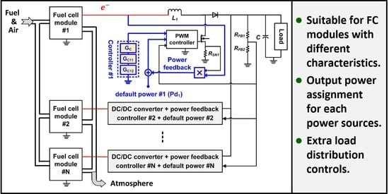
2.2. Proposed Power Sharing Control Configuration

Figure 3 presents the proposed method of connecting FC systems in parallel. Without loss of generality, two FCs are used as an example. Different from the current-feedback approach, the inner loop feeds back the power output of each FC, which is obtained by multiplying the FC’s voltage signal and current signal using a multiplier IC. Furthermore, two additional command inputs $\left(P{d}_1\mathrm{and}P{d}_2\right)$ are responsible for the power assignment in a rated condition. The aforementioned power signal and command inputs are added together through an adder IC to determine the duty ratio of the PWM regulator. The controller design is divided into three phases: $Gc,$ $G{c}_{i1},$ and $G{c}_{i2}$. The $G{c}_{i1}$ controller is designed to equalize the performance of employed FCs. The $G{c}_{i2}$ controller is designed to allocate extra load to FC modules when the load changes. The $Gc$ controller is designed to regulate the load voltage for the whole system. If these controllers function properly, the power output of each FC would be the same as $P{d}_1\mathrm{and}P{d}_2$ in the rated condition, and the extra load will be distributed to the two FCs according to the ratio of $G{c}_{12}\mathrm{and}G{c}_{22}$. This feedback control architecture is engineered with the consideration of circuit implementation using commercial PWM regulator ICs. In addition, the design and operation of those controllers do not need the communication between FCs. Therefore, the complexity of the control circuit is less and the whole system is reliable.

3. Dynamics Modeling

Most modeling of DC/DC converters is for current-feedback, single, and voltage sources. Hence, a mathematical model is developed for a power-feedback DC/DC converter with two FCs connected in parallel.

3.1. Fuel Cell

3.1.1. Dynamic Characteristics Modeling

The pressure and mass of gas in the gas channel can be described using the ideal gas law and the law of conservation of mass [24]:

$$\frac{d{p}_i}{dt}=\frac{R}{N_0{V}_j}\left(n_i\frac{d{T}_{cell}}{dt}+T_{cell}\frac{d{n}_i}{dt}\right)$$

(1)

$$\frac{d{n}_i}{dt}={\dot{n}}_{i,in}-{\dot{n}}_{i,out}-{\dot{n}}_{i,react}$$

(2)

where $N_0$ is the number of cell in a FC module; $p_i$ and $n_i$ are the partial pressure and mass of gas $i$ in the channel $j$; $R$ is the gas constant; $V_j$ is the volume of channel $j$; $T_{cell}$ is the cell temperature; ${\dot{n}}_{i,in}$, ${\dot{n}}_{i,out}$, ${\dot{n}}_{i,react}$ are the inlet, outlet, and reactive mass flow rate of gas $i$, respectively; and ${\dot{n}}_{i,out}$ is determined by the partial pressure of gas $i$ in the channel $j$.

The cell temperature can be described using the energy conservation law as follows:

$$\frac{d{T}_{cell}}{dt}=\frac{1}{N_0{m}_{cell}{C}_{p,cell}}\left({\dot{Q}}_{in}-{\dot{Q}}_{out}-{\dot{Q}}_{react}-P_{cell}\right)$$

(3)

where $m_{cell}$ and $C_{p,cell}$ are the equivalent mass and specific heat of cell; ${\dot{Q}}_{in}$, ${\dot{Q}}_{out}$, and ${\dot{Q}}_{react}$ are the heat carried by the inlet gas and outlet gas and chemical reaction, respectively; $P_{cell}$ is the electrical output power of cell.

3.1.2. Electrochemical Reaction Modeling

The ideal output voltage of the FC ($V_{ideal}$) can be described using the Nernst Equation [24,25]:

$$V_{ideal}=N_o\left[\frac{-∆g}{2F}+\frac{R{T}_{cell}}{2F}ln\left(\frac{p_{H_2}{p}_{O_2}^{0.5}}{p_{H_{2}O}}\right)\right]$$

(4)

where $-∆g$ is the Gibbs free energy; $F$ is the Faraday constant; $p_{H_2}$, $p_{H_{2}O}$, and $p_{O_2}$ are the partial pressures of hydrogen, steam, and oxygen, respectively. Due to various loss mechanisms, the output voltage of the cell is modelled as follows:

$$V_{cell}=V_{ideal}-V_{act}-V_{ohm}-V_{conc}$$

(5)

$$V_{act}=\gamma +\beta log\left(I_{cell}\right)$$

(6)

$$V_{ohm}=r_{0}exp\left[\alpha \left(\frac{1}{T_0}-\frac{1}{T_{cell}}\right)\right]·I_{cell}$$

(7)

$$V_{conc}=\frac{R{T}_{cell}}{2F}ln\left(\frac{I_{limit}}{I_{limit}-I_{cell}}\right)$$

(8)

where $V_{cell}$ is the output voltage of cell; $V_{act}$ the activation polarization; $V_{ohm}$ the ohmic polarization; and $V_{conc}$ the concentration polarization; $\mathsf{\gamma }$ and $\mathsf{\beta }$ are the Tafel constant and the Tafel slope constant, respectively; $r_0$ is the internal resistance at temperature $T_0$; $\alpha$ is a constant of the ohmic polarization; $I_{cell}$ and $I_{limit}$ are the cell output current and its maximum value, respectively; The gases in the anode channel include hydrogen and steam; the gases in the cathode channel only include oxygen. Using Equations (1)–(3) one can obtain the partial pressure of each gas in the channel, and the temperature of the cell. These numbers are fed into Equations (5)–(8) to calculate the output voltage of cell.

For the ease of the controller development, the static I–V characteristics of the FC are approximated using the following equations:

$$V_{cell}=a-k·I_{cell}$$

(9)

$$P_{cell}=\left(a-k·I_{cell}\right)·I_{cell}$$

(10)

where $a$ mimics the ideal voltage of FC; $k$ models the slope of I–V curve due to the aforementioned polarizations.

3.2. DC/DC Converters in Parallel

Assuming that the first set of the PWM regulator is working at a duty cycle $D_1$ and the second set of the PWM regulator at a duty cycle $D_2$, the unsynchronized switch of two PWM regulators results in three different circuit states, as shown in Figure 4. Because the switching speed of the PWM regulator is much faster than the overall system response, the time-averaging theorem is applied to model its performance [26]. The response of two DC/DC converters in parallel is derived as follows:

$$V_{cel{l}_1}=L_1\frac{d{I}_{cel{l}_1}}{dt}+\left(1-D_1\right)V_{load}$$

(11)

$$V_{cel{l}_2}=L_2\frac{d{I}_{cel{l}_2}}{dt}+\left(1-D_2\right)V_{load}$$

(12)

$$\frac{V_{load}}{R_{load}}=\left(1-D_1\right)I_{cel{l}_1}+\left(1-D_2\right)I_{cel{l}_2}-C\frac{d{V}_{load}}{dt}$$

(13)

where $V_{cell}$ and $I_{cell}$ are the averaged output voltage and current of a FC in a switch cycle, respectively; and $V_{load}$ the averaged voltage at the load terminal in a switch cycle.

3.3. PWM Regulator with Power Feedback

Inside the PWM chip (Figure 5a), there exists an internal oscillator that determines the clock rate of the PWM signal. In addition, a comparator compares the output from the controller ($v_{CONT}$) and the inner loop feedback signal ($v_{F,I}$), which in turn determines the duty ratio of the PWM signal. The controller is realized using a transimpedance amplifier and external circuit components. Assuming that the transimpedance gain is $g_m$ and the impedance of the external components is $Z_C$, the control signal ($v_{CONT}$) can be obtained as follows:

$$v_{CONT}=g_m\left(V_{ref}-v_{F,O}\right)\frac{R_o·Z_C}{R_o+Z_C}$$

(14)

where $R_o$ is the output impedance of the transimpedance amplifier, and $v_{F,O}$ is the outer loop feedback signal. The comparator inside the PWM regulator can cause an unstable harmonic oscillation when the duty cycle is greater than 50%. To overcome this problem, the PWM regulator employs an additional slope compensation signal to suppress it [27,28]. A geometrical relationship between these signals is shown in Figure 5b, and can be expressed as follows:

$$v_{F,I}=v_{CONT}-m_c·D{T}_s-\frac{1}{2}{m}_p·D{T}_s$$

(15)

where $T_s$ is the period of a switch cycle, $m_p$ the slope of the signal $v_{F,I}$, and $m_c$ the slope of the aforementioned internal compensation. In the proposed method, the input signal $v_{F,I}$ is from power feedback, and its slope ($m_p$) can be derived as follows:

$$v_{F,I}=\left(P_{cell}-P_d\right)·R_{SN}$$

(16)

$$m_p=\frac{\mathrm{d}{v}_{F,I}}{\mathrm{dt}}=R_{SN}\left(a-2k·I_{cell}\right)\frac{V_{cell}}{L}$$

(17)

3.4. Modeling of Two Fuel Cells and DC/DC Converters in Parallel

Because the circuit contains nonlinear components, the system model is derived for both the large- and small-signal models. The large-signal model describes the operation point of the circuit, whereas the small-signal model describes the dynamics of the circuit around that operation point. These signal models are obtained as follows: $(·)=\overline{(·)}+\widetilde{(·)}$, where $(·)$ denotes the time averaged signal in one switch cycle, $\overline{(·)}$ the DC value of the signal, and $\widetilde{(·)}$ the AC value of the signal [29]. Applying this method for Equations (9)–(17), the system model can be obtained as follows:

Large-signal model:

$${\overline{V}}_{cel{l}_i}=\left(1-{\overline{D}}_i\right){\overline{V}}_{load},i=1,2$$

(18)

$${\overline{V}}_{cel{l}_i}=a_i-k_i·{\overline{I}}_{cel{l}_i},i=1,2$$

(19)

$${\overline{P}}_{cel{l}_i}={\overline{V}}_{cel{l}_i}·{\overline{I}}_{cel{l}_i},i=1,2$$

(20)

$${\overline{m}}_{p_i}=\frac{R_{SN}}{L_i}\left(a_i-2k_i·{\overline{I}}_{cel{l}_i}\right){\overline{V}}_{cel{l}_i},i=1,2$$

(21)

$${\overline{D}}_i=\frac{1}{\left(m_{c_i}+\frac{1}{2}{\overline{m}}_{p_i}\right)T_s}\left({\overline{v}}_{CON{T}_i}+R_{SN}{P}_{d_i}-R_{SN}{\overline{P}}_{cel{l}_i}\right),i=1,2$$

(22)

$$\frac{{\overline{V}}_{load}}{R_{load}}={\displaystyle \sum }_{i=1}^2\left(1-{\overline{D}}_i\right){\overline{I}}_{cel{l}_i},i=1,2$$

(23)

Small-signal model:

$$G_{PBC}:\left[\begin{array}{c}{\stackrel{·}{\tilde{I}}}_{cel{l}_1}\\ {\stackrel{·}{\tilde{I}}}_{cel{l}_2}\\ {\stackrel{·}{\tilde{V}}}_{load}\end{array}\right]=\left[\begin{array}{ccc}\frac{-k_1}{L_1}& 0& \frac{-(1-{\overline{D}}_1)}{L_1}\\ 0& \frac{-k_2}{L_2}& \frac{-(1-{\overline{D}}_2)}{L_2}\\ \frac{(1-{\overline{D}}_1)}{C}& \frac{(1-{\overline{D}}_2)}{C}& \frac{-1}{R_{1oad}C}\end{array}\right]\left[\begin{array}{c}{\tilde{I}}_{cel{l}_1}\\ {\tilde{I}}_{cel{l}_2}\\ {\tilde{V}}_{load}\end{array}\right]\left[\begin{array}{cc}\frac{{\overline{V}}_{load}}{L_1}& 0\\ 0& \frac{{\overline{V}}_{load}}{L_2}\\ \frac{-{\overline{I}}_{cel{l}_1}}{C}& \frac{-{\overline{I}}_{cel{l}_2}}{C}\end{array}\right]\left[\begin{array}{c}{\tilde{D}}_1\\ {\tilde{D}}_2\end{array}\right]$$

(24)

$${\tilde{V}}_{cel{l}_i}=-k_i·{\tilde{I}}_{cel{l}_i},i=1,2$$

(25)

$${\tilde{P}}_{cel{l}_i}=\left(a_i-2k_i·{\overline{I}}_{cel{l}_i}\right)·{\tilde{I}}_{cel{l}_i},i=1,2$$

(26)

$${\tilde{m}}_{p_i}=R_{SN}\left(\frac{-2k_i}{L_i}{\overline{V}}_{cel{l}_i}-\frac{a_i-2k_i{\overline{I}}_{cel{l}_i}}{L_i}{k}_i\right)·{\tilde{I}}_{cel{l}_i},i=1,2$$

(27)

$${\tilde{D}}_i=\frac{1}{\left(m_c+\frac{1}{2}{\overline{m}}_{p_i}\right)T_s}\left({\tilde{v}}_{CON{T}_i}-R_{SN}{\widehat{P}}_{cel{l}_i}-\frac{1}{2}{\overline{D}}_i{T}_s{\tilde{m}}_{p_i}\right),i=1,2$$

(28)

4. Controller Design

According to the small-signal model shown in Equations (24)–(28), the dynamics of the two FCs along with converters are coupled together, particularly at the plant $G_{PBC}$ shown in Equation (24). For the ease of controller design, we define new state ${\tilde{V}}_{loa{d}_i}$ which is the load voltage variation of the i-th FC due to the current variation of the cell itself (${\tilde{I}}_{cel{l}_i}$). In this case, ${\tilde{V}}_{load}={\tilde{V}}_{loa{d}_1}+{\tilde{V}}_{loa{d}_2}$. Furthermore, Equation (24) can be rewritten as follows:

$$G_{PBC}:\left[\begin{array}{c}{\dot{\tilde{I}}}_{cel{l}_1}\\ {\dot{\tilde{I}}}_{cel{l}_2}\\ {\dot{\tilde{V}}}_{loa{d}_1}\\ {\dot{\tilde{V}}}_{loa{d}_2}\end{array}\right]=\left[\begin{array}{cccc}\frac{-k_1}{L_1}& 0& \frac{-\left(1-{\overline{D}}_1\right)}{L_1}& \frac{-\left(1-{\overline{D}}_1\right)}{L_1}\\ 0& \frac{-k_2}{L_2}& \frac{-\left(1-{\overline{D}}_2\right)}{L_2}& \frac{-\left(1-{\overline{D}}_2\right)}{L_2}\\ \frac{\left(1-{\overline{D}}_1\right)}{C}& 0& \frac{-1}{R_{load}C}& 0\\ 0& \frac{\left(1-{\overline{D}}_2\right)}{C}& 0& \frac{-1}{R_{load}C}\end{array}\right]·\left[\begin{array}{c}{\tilde{I}}_{cel{l}_1}\\ {\tilde{I}}_{cel{l}_2}\\ {\tilde{V}}_{loa{d}_1}\\ {\tilde{V}}_{loa{d}_2}\end{array}\right]+\left[\begin{array}{cc}\frac{{\overline{V}}_{load}}{L_1}& 0\\ 0& \frac{{\overline{V}}_{load}}{L_2}\\ \frac{-{\overline{I}}_{cel{l}_1}}{C}& 0\\ 0& \frac{-{\overline{I}}_{cel{l}_2}}{C}\end{array}\right]\left[\begin{array}{c}{\tilde{D}}_1\\ {\tilde{D}}_2\end{array}\right]$$

(29)

From the equation above, two subsystem $G_{PBC,1}$ and $G_{PBC,2}$ are defined to describe the dynamics of $G_{PBC}$.

$$G_{PBC,1}:\left[\begin{array}{c}{\dot{\tilde{I}}}_{cel{l}_1}\\ {\dot{\tilde{V}}}_{loa{d}_1}\end{array}\right]=\left[\begin{array}{cc}\frac{-k_1}{L_1}& \frac{-\left(1-{\overline{D}}_1\right)}{L_1}\\ \frac{\left(1-{\overline{D}}_1\right)}{C}& \frac{-1}{R_{load}C}\end{array}\right]·\left[\begin{array}{c}{\tilde{I}}_{cel{l}_1}\\ {\tilde{V}}_{loa{d}_1}\end{array}\right]\left[\begin{array}{c}\frac{{\overline{V}}_{load}}{L_1}\\ \frac{-{\overline{I}}_{cel{l}_1}}{C}\end{array}\right]·{\tilde{D}}_i+\frac{-\left(1-{\overline{D}}_1\right)}{L_1}{\tilde{V}}_{loa{d}_2}$$

(30)

$$G_{PBC,2}:\left[\begin{array}{c}{\dot{\tilde{I}}}_{cel{l}_2}\\ {\dot{\tilde{V}}}_{loa{d}_2}\end{array}\right]=\left[\begin{array}{cc}\frac{-k_2}{L_2}& \frac{-\left(1-{\overline{D}}_2\right)}{L_2}\\ \frac{\left(1-{\overline{D}}_2\right)}{C}& \frac{-1}{R_{load}C}\end{array}\right]·\left[\begin{array}{c}{\tilde{I}}_{cel{l}_2}\\ {\tilde{V}}_{loa{d}_2}\end{array}\right]\left[\begin{array}{c}\frac{{\overline{V}}_{load}}{L_2}\\ \frac{-{\overline{I}}_{cel{l}_2}}{C}\end{array}\right]·{\tilde{D}}_2+\frac{-\left(1-{\overline{D}}_2\right)}{L_2}{\tilde{V}}_{loa{d}_1}$$

(31)

In order to obtain a graphical representation of the system dynamics, we define two function blocks $G_{m,i1}$ and $G_{m,i2}$ for the PWM dynamics shown in Equations (27) and (28).

$${\tilde{D}}_i=G_{m,i2}\left({\tilde{v}}_{CON{T}_i}+G_{m,i1}·{\tilde{I}}_{cel{l}_i}\right),i=1,2$$

(32)

$$G_{m,i1}=R_{SN}\left[-a_i+2k_i·{\overline{I}}_{cel{l}_i}+\frac{{\overline{D}}_i{T}_s{k}_i}{L_i}\left({\overline{V}}_{cel{l}_i}+0.5a_i-k_i·{\overline{I}}_{cel{l}_i}\right)\right],\hspace{1em}i=1,2$$

(33)

$$G_{m,i2}=\frac{1}{\left(m_c+\frac{1}{2}{\overline{m}}_{p_i}\right)T_s},\hspace{1em}i=1,2$$

(34)

Figure 6 shows the block diagram of the overall system when including the controller designs mentioned previously. To further simplify the notation, we define the transfer function $G_{p1}$ which has the input signal of ${\tilde{v}}_{CONT,1}$ and the output signal ${\tilde{V}}_{load,1}\left(t\right)$, when ${\tilde{V}}_{load,2}$ is zero. $G_{p2}$ is defined analogously. Therefore, $G_{p1}$ and $G_{p2}$ are two decoupled subsystems.

The design of the $Gc$ controller is to ensure that the outer loop has a large gain in the low-frequency region and that the bandwidth of the outer loop is much smaller than the bandwidth of $G_{P1}$ and $G_{P2}$. The requirement of the “large gain” is to ensure that the ${\tilde{V}}_{load}$ is small, so are the ${\tilde{V}}_{loa{d}_1}$ and ${\tilde{V}}_{loa{d}_2}$. Therefore, the coupled dynamics can be approximated by two decoupled subsystems $G_{P1}$ and $G_{P2}$. The requirement of the “smaller bandwidth” is to set design guidelines for the $G_{C11}$ and $G_{C21}$ controllers so that they can be implemented using low-order transfer functions. The reason for this will be elaborated in Section 7.

The controllers $G_{C11}$ and $G_{C21}$ are designed to compensate the transient response of two independent subsystems $G_{P1}$ and $G_{P2}$ to ensure that both channels ($G_{C11}·G_{P1}$ and $G_{C21}·G_{P2}$) have the similar response in the low-frequency region, which region is defined by the $Gc$ controller.

The controllers $G_{C12}$ and $G_{C22}$ are two constants. Their values determine the response time of each parallel-connected channel ($G_{C12}·G_{C11}·G_{P1}$ and $G_{C22}·G_{C21}·G_{P2}$), which in turn determines the distribution ratio of the extra load when the system is subjected to load changes. In a special case of the minimum-power-variation ratio (MPVR) for the extra load distribution, $G_{C12}$ and $G_{C22}$ values can be derived by solving the following Lagrange equation:

$$H=-\frac{1}{2}∆p_1^2-\frac{1}{2}∆p_2^2+\lambda \left(∆P_{load}-P_{cel{l}_1}∆p_1-P_{cel{l}_2}∆p_2\right)$$

(35)

where $∆p_1\mathrm{and}∆p_2$ are the percentage of the power variation of each source; $∆P_{load}$ the load variation; and $\lambda$ the Lagrange multiplier. After applying the optimization method to solve Equation (35), $∆p_1$ and $∆p_2$ can be obtained as follows:

$$∆p_1=\frac{p_{cel{l}_1}^2}{p_{cel{l}_1}^2+p_{cel{l}_2}^2}$$

(36)

$$∆p_2=\frac{p_{cel{l}_2}^2}{p_{cel{l}_1}^2+p_{cel{l}_2}^2}$$

(37)

$G{c}_{11}$ and $G{c}_{21}$ are chosen to be the same as $∆p_1$ and $∆p_2$ to achieve the MPVR for the extra load distribution.

5. Simulation Results

The parameters of the converter and load impedance are shown in

Table 1. Parameters of the boost converters and load impedance.

Symbol	Value	Symbol	Value
$L_1$	$50\mathsf{\mu }\mathrm{H}$	$R_{load}$	$12.5\mathsf{\Omega }$
$L_2$	$50\mathsf{\mu }\mathrm{H}$	$R_{sn}$	$0.15\mathsf{\Omega }$
$C$	$150\mathsf{\mu }\mathrm{F}$	$g_m$	$8\times {10}^{-4}{\mathsf{\Omega }}^{-1}$
$R_{FB1}$	$70\mathrm{k}\mathsf{\Omega }$	$R_o$	$47.5\mathrm{k}\mathsf{\Omega }$
$R_{FB2}$	$10\mathrm{k}\mathsf{\Omega }$	$f_{sw}$	$200\mathrm{kHz}$

. These component values were used both in the simulations and experiments.

5.1. Parallel Performance of Fuel Cells with Different Cell Characteristics

In this simulation, two FCs were connected in parallel using the conventional methods shown in Figure 2. Because the response of the power electronics is much faster than that of the FC, the dynamics of the power electronics was ignored and the integrated system was modeled as shown in Figure 7. In this simulation, the load power is 10 W, and the flow rates of hydrogen and oxygen are 0.0017 and 0.0035 mole s⁻¹, respectively. To illustrate the effect of employed FCs having different characteristics, two FCs are assumed to have the same characteristics before $4\times {10}^3$ s, but differs in their internal resistance ($r_0$ in Equation (7)) after $4\times {10}^3$ s.

Table 2. Parameter values used at different FCs.

Symbol	Value	Symbol	Value
$m_{cell}$	$16.5\mathrm{g}$	$N_o$	$8\left(\mathrm{each}\mathrm{module}\right)$
$V_{anode}$	$0.006{\mathrm{m}}^3$	$C_{p, cell}$	$0.4{\mathrm{J}\mathrm{g}}^{-1}{\mathrm{K}}^{-1}$
$V_{cathode}$	$0.002{\mathrm{m}}^3$	$∆g$	$-242,872.9+48.63\times T_{cell}$
$\gamma$	$0.05$	${\dot{n}}_{H_2,in}$	$0.0017{\mathrm{mole}\mathrm{s}}^{-1}$
$\beta$	$0.11$	${\dot{n}}_{H_{2}O,in}$	$0{\mathrm{mole}\mathrm{s}}^{-1}$
$\alpha$	$-2870$	${\dot{n}}_{O_2,in}$	$0.0035{\mathrm{mole}\mathrm{s}}^{-1}$
$T_0$	$1273.15\mathrm{K}$	$I_{limit}$	$0.8{\mathrm{A}\mathrm{cm}}^2$
$r_0$	$\{\begin{array}{c}\mathrm{time}<4\times {10}^3: \mathrm{FC} \#1=\mathrm{FC} \#2=25 \mathsf{\Omega }\\ \mathrm{time}\ge 4\times {10}^3: \mathrm{FC} \#1=25 \mathsf{\Omega }, \mathrm{FC} \#2=150 \mathsf{\Omega }\end{array}$

lists all the parameters of FCs used in this simulation. These parameters can be obtained from published articles [24,25], except the internal resistance.

Figure 8 shows the output power (left plot) and temperature response (right plot) of each cell, where the FC #1 is drawn in blue and FC #2 drawn in dashed green lines. According to the simulation results, the temperature response and power sharing of two FCs before $4\times {10}^3$ s are exactly the same. However, the power sharing of FC #1 and FC #2 at $4.1\times {10}^3$ s is 6.5 and 1.1 W, the corresponding temperatures are respectively 908 and 956 K, and they diverge afterwards. This thermal runaway can be accounted as: less power output leading to higher cell temperature, in turns larger voltage loss and lower power output. As suggested by the results, the parallel-connected FC system can be notably altered by FCs with different characteristics and the conventional method cannot solve this issue.

5.2. Performance of Proposed Control Method

To focus on the controller design of the proposed method, the static I-V curves of above two FCs (parameters listed in Table 2) were obtained and approximated for the following simulations. Figure 9 shows the comparison of the fuel cell models from Equations (1)–(8) and the approximate models (Equations (38) and (39)). The corresponding I–V curves are shown in the plot on the left, the I–P curves are on the right. According to the plot, the approximate models are close to the electrical characteristics of the fuel cell modules.

$$V_{cel{l}_1}=7-0.5·I_{cel{l}_1}$$

(38)

$$V_{cel{l}_2}=7-1·I_{cel{l}_2}$$

(39)

5.2.1. Controller Design

In this case, the designated power outputs of FC #1 and #2 were 4.8 and 3.2 W, respectively. The bode plot of the uncompensated FC and DC/DC converter ($G_{p1}$ and $G_{p2}$ in Figure 6) were drawn in blue dashed and green dashed lines in the right column of Figure 10. From the figure, the uncompensated FCs had different response in the low frequency region, which difference was approximately $0.8\mathrm{dB}$. Controllers $G_{C11}$ and $G_{C21}$ were designed to be 1 and 1.096 to equalize this difference. After the compensation, these two channels ($G_{c11}·G_{p1}$ in the blue line and $G_{c21}·G_{p2}$ in the green-dash line shown in the right column of Figure 10) had the same frequency response below 275 Hz. The $G_c$ controller was designed to largely attenuate the response of $G_{c11}·G_{p1}$ and $G_{c21}·G_{p2}$ above 275 Hz. The controller $G_c$ was designed as $\left(0.02s+8\right)/\left(s+10\right)$ where the pole of 10 rad/s was for the high-frequency attenuation, the zero of the transfer function came from the output impedance of the transimpedance amplifier (see Equation (14)). The distribution controllers $G_{c12}$ and $G_{c22}$ were 0.6923 ($={4.8}^2/\left({4.8}^2+{3.2}^2\right)$) and 0.3077 ($={3.2}^2/\left({4.8}^2+{3.2}^2\right)$) for the MPVR distribution. The Bode plot of the overall system (including the voltage gain set by the resistors in the feedback loop), drawn in red, had a bandwidth of 1.6 Hz. More of the design considerations are explained in Section 7.

5.2.2. Power Assignment

By using the proposed controllers, the system response for different power assignments was simulated. In case 1 (left column in Figure 11), the control parameters were ($P_{d1}$, $P_{d2}$) = (4.8, 3.2), with the designated power outputs being 4.8 and 3.2 W, respectively. In case 2 (right column in Figure 11), the control parameters were ($P_{d1}$, $P_{d2}$) = (4, 4). According to the simulation results shown in Figure 11, the load voltage was 9.7 V, and the total power output was approximately 7.5 W in both cases. The load power did not reach the designated value due to the error of the load voltage, which will be discussed in Section 7. To evaluate the performance of the proposed method and exclude effects such as the power efficiency and control inaccuracy of the converter, we scaled the output power of each source before using it to calculate the relative error of the power assignment. This scale factor (SF) and the corresponding relative error of the power assignment are defined as follows:

$$\mathrm{SF}\triangleq \frac{designatedloadpower}{totalpoweroutput}$$

(40)

$$\mathrm{Relative}\mathrm{error}\triangleq \frac{\left(poweroutput\right)\times SF-P_d}{P_d}\times 100\%$$

(41)

According to the simulation results, the power sharing was (4.5 W, 3 W) in case 1. The SF was 1.07 (=$\left(4.8+3.2\right)/\left(4.5+3\right)$), and the relative errors of the power assignment were both 0% of source 1 and 2. In case 2, the power sharing was (3.75 W, 3.75 W). The SF was also 1.07 (=$\left(4+4\right)/\left(3.75+3.75\right)$), and the relative errors of the power assignment were both 0% of source 1 and 2. Therefore, the proposed method can assign different power sharing in the rated condition.

5.2.3. Extra Load Distribution

In this simulation, the extra load distribution was verified for the system subjected to a load change. The control parameters were ($P_{d1}$, $P_{d2}$) = (4.8, 3.2). The load resistor ($R_{load}$) varied from $12.5$ to $10\mathsf{\Omega }$ at 0.1 s, which corresponds to an output power from 8 to 10 W. In case 1, the distribution controllers $G_{c12}$ and $G_{c22}$ were both 0.5, and the extra load 2 W (=$10-8 \mathrm{W}$) should be equally shared by the two FCs. In case 2, $G_{c12}$ and $G_{c22}$ were 0.6923 and 0.3077, and the extra load should be shared by the two FCs at a 0.6923:0.3077 ratio. Figure 12 shows the simulation results of case 1 (left column) and case 2 (right column). According to the results, the output voltage switched from 9.7 to 9.4 V, which corresponded to an output power variation from 7.5 to 8.8 W. Again, the power assignment performance was evaluated using Equations (40) and (41). In case 1, the output power of the two FCs varied from (4.5 W, 3 W) to (5.1 W, 3.7 W). Before the load variation, the power distribution ratio was 0.6:0.4. After the load variation, FC #1 and #2 increased 0.6 and 0.7 W, respectively, the distribution ratio of extra load being 0.4615:0.5385, with the ratio error being 3.85%. In case 2, the output power of the two FCs varied from (4.8 W, 2.7 W) to (5.7 W, 3.1 W). Before the load variation, the SF was 1.07 (=$\left(4.8+3.2\right)/\left(4.8+2.7\right)$), and the relative error of the power assignment was 6.67% of source 1 and −10% of source 2. After the load variation, FC #1 and #2 increased 0.9 and 0.4 W, respectively, the distribution ratio of extra load being 0.6923:0.3077, which was the same as the designated value. These results indicated that the distribution controller can distribute the extra load as requested, and different distribution controllers interfered minorly the power output in the rated conditions.

6. Experimental Results

6.1. Layout of the Experimental Circuit

A PWM regulator LM3478 (Texas Instruments, Dallas, TX, USA) was used to experimentally test the proposed control method. For proof of concept, circuits with FC-like I–V characteristics were used to replace the FC in the experiments. The experiments were conducted at a load voltage of 10 V and a power of 10 W, which were the same as those in the simulations.

As explained previously, two controllers were used: $Gc·G{c}_{11}·G{c}_{12}$ and $Gc·G{c}_{21}·G{c}_{22}$. Without loss of generality, these two controllers were implemented with $Gc$ and $Gc·\left(G{c}_{21}·G{c}_{22}\right)/\left(G{c}_{11}·G{c}_{12}\right)$, as shown in Figure 13. Owing to the low-bandwidth design of the $G_C$ controller, $\left(G{c}_{21}·G{c}_{22}\right)/\left(G{c}_{11}·G{c}_{12}\right)$ could be a scalar. And, its magnitude was intentionally designed to be smaller than one to ensure that both controllers could be implemented using passive electronic components. For instance, if $C_{C1}$ and $R_{C1}$ were used to realize $Gc$, $Gc·\left(G{c}_{21}·G{c}_{22}\right)/\left(G{c}_{11}·G{c}_{12}\right)$ could be realized by the circuit drawn in Figure 13, where $R_{o1}=b·R_o,C_{C2}=1/b·C_{C1},R_{C2}=b·R_{C1}$, and “$b$” is derived as follows:

$$b=\frac{{Gc}_{21}·{Gc}_{22}}{{Gc}_{11}·{Gc}_{12}-{Gc}_{21}·{Gc}_{22}}$$

(42)

In the following experiments, $R_{c1}=1\mathrm{k}\mathsf{\Omega },C_{C1}=2.2\mathsf{\mu }\mathrm{F}$, $G_C\left(s\right)\cong 38·\left(0.02s+9.37\right)/\left(s+9.37\right)$ can be calculated using Equation (14). The parameter “$b$” for realizing the controller $Gc·\left(G{c}_{21}·G{c}_{22}\right)/\left(G{c}_{11}·G{c}_{12}\right)$ would be calculated based on the distribution controller in each experiment.

Figure 14 illustrates two sets of circuits that can mimic the I–V characteristics of the FC. The parameters of the circuit are $R_{11}=R_{12}=10\mathrm{k}\mathsf{\Omega }$, $R_{13}=R_{14}=5\mathrm{k}\mathsf{\Omega }$, $R_{15}~R_{18}=10\mathrm{k}\mathsf{\Omega }$, $R_{21}~R_{28}=10\mathrm{k}\mathsf{\Omega }$, $R_{d1}=R_{d2}=1\mathsf{\Omega }$, $V_{s1}=V_{s2}=10\mathrm{V}$, and $a_1=a_2=7\mathrm{V}$.

The experimental results are presented in Figure 15. These two circuits demonstrated different FC-like I-V characteristics. After curve fitting, their I–V characteristics was calibrated as follows:

$$V_{cell1}=7.03-0.46·I_{cell1}$$

(43)

$$V_{cell2}=7.01-0.96·I_{cell2}$$

(44)

6.2. Power Assignment and Extra Load Distribution

Figure 16 presents the experimental results of the proposed control circuit (Figure 13) using the two FC-like sources (Figure 14). In this experiment, the designated power output was 4 W for each source, and the extra load distribution ratio was 0.5:0.5.

According to the results, in the rated condition (8-W load), source 1 had an output of 6.625 V and 0.7866 A (Figure 16a), source 2 had an output of 6.226 V and 0.733 A (Figure 16b), and the load voltage was approximately 10.2 V. Therefore, the output powers of sources 1 and 2 were 5.21 (=$6.625\times 0.7866$) and 4.56 W (=$6.226\times 0.733$), respectively. The power delivered to the load was 8.32 W (=$V_{load}^2/R_{load1}={10.2}^2/12.5$). Similarly, in the load variation case (10-W load), source 1 had an output of 6.56 V and 0.9204 A (Figure 16c), source 2 had an output of 6.033 V and 0.9136 A (Figure 16d), and the load voltage was 10.08 V. The output powers of sources 1 and 2 were 6.04 and 5.51 W, respectively. The power delivered to the load was 10.2 W ($=V_{load}^2/\left(R_{load1}//R_{load2}\right)={10.08}^2/10$).

Before the load variation, the SF was 0.82 (=$8/\left(5.21+4.56\right)$) using Equations (40) and (41). The relative error of the power assignment was 6.62% of source 1 and −6.62% of source 2. After the load variation, Source 1 increased 0.83 W (=6.04 − 5.21), and source 2 increased 0.95 W (=5.51 − 4.56). The distribution ratio of the extra load was 0.466:0.534 (=$0.83/\left(0.83+0.95\right):0.95/\left(0.83+0.95\right)$). Therefore, the distribution error was 3.4%. According to these results, the proposed method can distribute the load both in the rated condition and in the load change. In the subsequent experiment, the power assignments were 4.8 and 3.2 W for sources 1 and 2 in the rated condition, and a ratio of 0.5:0.5 was employed for the extra load distribution in the load variation case. The controllers remained the same. According to the experimental results in Figure 17, in the rated condition, source 1 had an output of 6.65 V and 0.8505 A (Figure 17a), source 2 had an output of 6.45 V and 0.5338 A (Figure 17b), and the load voltage was 10.12 V. The output powers of sources 1 and 2 were 5.656 and 3.443 W, respectively.

Using Equations (40) and (41), the relative error of the power assignment was 3.69% of source 1 and −5.32% of source 2. In the 10-W case (load variation), source 1 had an output of 6.556 V and 1.049 A (Figure 17c), source 2 had an output of 6.192 V and 0.7615 A (Figure 17d), and the load voltage was 10.07 V. Therefore, the power outputs of sources 1 and 2 were 6.877 and 4.715 W, respectively. Due to the load variation, the output power of sources 1 and 2 increased by 1.221 and 1.272 W, respectively. The distribution ratio of the extra load was calculated as 0.490:0.510, using the same method shown in the previous case. Therefore, the distribution error was 1%. This experiment indicated that different command inputs ${\mathrm{P}}_{\mathrm{d}}$ can assign different power sharing in the rated condition without interfering the distribution ratio in the load change.

6.3. MPVR Distribution

In this experiment, the power assignment in the rated condition was the same as in Figure 17. However, the extra load distribution ratio was 0.6923:0.3077$(={4.8}^2/\left({4.8}^2+{3.2}^2\right):{4.8}^2/\left({4.8}^2+{3.2}^2\right)$ for the MPVR; therefore, “$b$” = 0.8 in Equation (40). According to the experimental results in Figure 18, in the rated condition, source 1 had an output of 6.575 V and 0.8913 A (Figure 18a), source 2 had an output of 6.433 V and 0.5413 A (Figure 18b), and the load voltage was 10.1 V. The output powers of sources 1 and 2 were 5.86 and 3.482 W, respectively. Using Equations (40) and (41), the relative error of the power assignment was 4.99% of source 1 and −6.42% of source 2. In the 10-W case, source 1 had an output of 6.475 V and 1.096 A (Figure 18c), source 2 had an output of 6.293 V and 0.6751 A (Figure 18d), and the load voltage was 10.08 V. Therefore, the output powers of sources 1 and 2 were 7.097 and 4.248 W, respectively. Due to the load variation, the output power of source 1 increased by 1.237 W and of source 2 increased by 0.766 W. The distribution ratio of the extra load was calculated as 0.618:0.382. Therefore, the distribution error was 7.43%. This experiment indicated that different distribution controller can distribute the extra load as requested with minor interference on the power output in the rated conditions.

7. Discussion

Figure 11 presents the simulation results of different power assignments $\left(P_{d1},P_{d2}\right)$ when the distribution controllers ($G_{c12}$ and $G_{c22}$) were the same. By contrast, Figure 12 shows the simulation results of the same power assignments when the distribution controllers were different. Figure 16, Figure 17 and Figure 18 display the experimental results of three different combinations of power assignments and distribution controllers. According to the simulation and experimental results listed in

Table 3. Simulation and experimental results.

		Power Assignment (Output/Assignment)	Extra Load Dist. Ratio (Output/Assignment)	Power Assignment Error	Extra Load Dist. Error
Sim. 1	FC #1	4.5/4.8	0.4615/0.5	0%	3.85%
	FC #2	3/3.2	0.5385/0.5	0%
Sim. 2	FC #1	4.8/4.8	0.6923/0.6923	6.67%	0%
	FC #2	2.7/3.2	0.3077/0.3077	−10%
Exp. 1	FC #1	5.21/4	0.466/0.5	6.62%	3.4%
	FC #2	4.56/4	0.534/0.5	−6.62%
Exp. 2	FC #1	5.66/4.8	0.49/0.5	3.69%	1%
	FC #2	3.44/3.2	0.51/0.5	−5.32%
Exp. 3	FC #1	5.86/4.8	0.618/0.692	4.99%	7.43%
	FC #2	3.48/3.2	0.382/0.308	−6.42%

, the proposed method achieved a relative error less than 6.62% for the power assignment under rated conditions, and the ratio errors less than 7.43% for distributing the extra load. Therefore, the proposed method could regulate the power output of FC-like power sources in parallel.

As mentioned previously, different output power of a FC module corresponds to different operation point of the FC. The shift of the operation point, due to the load variation, can be related to the percentage of the power variation. That is why we proposed the MPVR controls in this paper. The percentage of the power variation of a system can be evaluated by $\sum _i\left|∆p_i\right|$. The difference of the experiments shown in Figure 17 and Figure 18 is the distribution ratio for the extra load, which one is equally distributed and one is distributed by the MPVR method. In the case of equally distributed (Figure 17), the percentage of the power variation is evaluated as follows:

$$\left|∆p_1\right|+\left|∆p_2\right|=\left|\frac{1.221}{5.656}\right|+\left|\frac{1.272}{3.443}\right|=0.585$$

(45)

In the case of MPVR method (Figure 18), the percentage of the power variation is evaluated as follows:

$$\left|∆p_1\right|+\left|∆p_2\right|=\left|\frac{1.237}{5.86}\right|+\left|\frac{0.766}{3.482}\right|=0.431$$

(46)

Therefore, under the same load changes, the proposed MPVR method achieved a smaller percentage of the power variation than other distribution ratios. Thus, the associated FCs may work close to their designated operation points even when the load changes.

In a parallel-connected power system, the power sharing is largely determined by the different response time of each module. That is why we proposed a control method that can engineers the bandwidth of each parallel-connected module of a dynamics coupled system, and achieves the power sharing without the communication between modules. However, the bandwidth of each module affects the power sharing both in the rated condition and load changes, which means that one cannot independently assign the power sharing for the rated conditions and extra load distribution. Conventional methods solve this problem by using the additional control inputs (ex. $P_d$ input in the proposed method) and much lowered bandwidth of the control loop. In contrast, the proposed method solves it by the nonlinearity of the PWM regulator, which will be explained shortly.

As aforementioned, the comparator inside the PWM chip compares the input signals of $v_{CONT}$ and $v_{F,I}$ to determine the duty ratio of the PWM signal. Therefore, it works under two phases:

$$\{\begin{array}{c}D=1,\left|\left(P_{cell}-P_d\right)·R_{SN}-v_{CONT}\right|>\left(m_c+\frac{1}{2}{m}_p\right)·D{T}_s\\ D=\frac{v_{CONT}-\left(P_{cell}-P_d\right)·R_{SN}}{\left(m_c+\frac{1}{2}{m}_p\right)·T_s},\left|\left(P_{cell}-P_d\right)·R_{SN}-v_{CONT}\right|\le (m_c+\frac{1}{2}{m}_p)·D{T}_s\end{array}$$

(47)

According to the equation above, the distribution controllers, which regulates the bandwidth of each parallel-connected module, are in effect only when the difference between $v_{CONT}$ and ($\left(P_{cell}-P_d\right)·R_{SN}$) is less than $\left(m_c+0.5·m_p\right)·D{T}_s$, whose value is equivalent to approximately 8 W in the case of 200 W load power. Therefore, the bandwidth would mostly affect load distribution when the load changes but not in the rated condition set by the control input $P_d$. This explains the results shown in Figure 12 and Figure 18 where the power sharing varies less than 7.43% in the rated condition but the bandwidth of two modules varies as much as 2.3 times (=0.6923/0.3077).

The nonlinearity of the PWM regulator also accounts for the outcome that the power sharing does not exactly meet the designated value ($P_d$) even under the rated condition. This is because the difference between $v_{CONT}$ and ($\left(P_{cell}-P_d\right)·R_{SN}$) determines the duty ratio of the PWM signal, which in turn determines the voltage amplification of the DC/DC converter. The feedback signal $v_{CONT}$ determined by the error voltage is small when the load voltage reaches its designated value. Therefore, according to Equation (47), ($P_{cell}-P_d$) $\cong \left(m_c+0.5·m_p\right)·D{T}_s\ne 0$, which implies that $P_{cell}\ne P_d$ in most cases. Nevertheless, this error is minor, especially in the large power systems, because the magnitude of $\left(m_c+0.5·m_p\right)·D{T}_s$ is small compared to the power output.

Equations (15) and (16) suggest that a large sense resistor $R_{SN}$ may be helpful to minimize the error of $\left(P_{cell}-P_d\right)$. Using a large sense resistor could be problematic due to the maximum current limitation mentioned in Section 2.1. However, this is not the case in the proposed method because its feedback signal is $\left(P_{cell}-P_d\right)·R_{SN}$, instead of $P_{cell}·R_{SN}$, and the $\left(P_{cell}-P_d\right)$ can be much smaller than $P_{cell}$. Therefore, the proposed method has an additional advantage that it can be applied to realize the control circuits for the large power systems without additional work on the sense resistor $R_{SN}$.

In order to experimentally verify the proposed method and minimize the uncertainties in experiments, we chose commercial LM3478 PWM chips to realize the circuits. Conversely, some features of the LM3478 impose constraints for the controller designs, which features include the output impedance of its transimpedance amplifier and the DC bias (~1.5 V) at its $v_{CONT}$ terminal. Due to the existence of the output impedance, the controller must have a zero but no integrator in its transfer function. Due to the existence of the DC bias, the controllers $Gc,$ $G{c}_{i1},$ and $G{c}_{i2}$ must be implemented together. Furthermore, no active electronic component is allowed to implement the controller. Consequently, the order of the transfer function $Gc·G_{Ci1}·G_{Ci2}$ is less than or equal to two, and the maximum gain is limited to $g_m{R}_o$. Owing to these limitations, in the current design, $G{c}_{i1}$ are chosen to be constant to compensate for the low-frequency response only, and the $Gc$ controller must have a compatible low-bandwidth property. In addition, it is difficult to further minimized the load voltage error, as shown in Figure 11 and Figure 12, because the controller gain is limited by $g_m{R}_o$.

8. Conclusions

In this paper, a novel control circuit for the parallel-connected FC power system was proposed. As shown in this paper, the performance of each FC module can be notably altered in a parallel-connected system when the employed FC modules have different characteristics. This circuit controls the performance (operating point) of each FC module by controlling the power assignment in rated conditions and allocation ratio of additional power when the load changes. This control circuit is developed from a proposed control method that includes controllers, power-feedback DC/DC converter, and additional command inputs. The controller design is divided into three steps; each step has been discussed in detail herein. Finally, two FC-like sources were implemented to experimentally evaluate the performance of the proposed control method.

Nonlinearity of the PWM regulator is the key to this design. It enables the proposed power-sharing method without compromising the bandwidth of the system response. The experimental results agree well with the simulation results. Both results indicated that the power assignment under the rated condition had a relative error of less than 6.62%. The distribution ratio error under the load change was less than 7.43%. Therefore, the proposed method can regulate the power output of each parallel-connected FC-like power source.

References

1. Chang, H.; Lee, I.H. Environmental and efficiency analysis of simulated application of the solid oxide fuel cell co-generation system in a dormitory building. Energies 2019, 12, 3893. [Google Scholar] [CrossRef] [Green Version]
2. Chatillon, Y.; Bonnet, C.; Lapicque, F. Heterogeneous aging within PEMFC stacks. Fuel Cells 2014, 14, 581–589. [Google Scholar] [CrossRef]
3. Wu, C.C.; Chen, T.L. Dynamic modeling of a parallel-connected solid oxide fuel cell stack system. Energies 2020, 13, 501. [Google Scholar] [CrossRef] [Green Version]
4. Chippar, P.; Ko, J.; Ju, H. A global transient, one-dimensional, two-phase model for direct methanol fuel cells (DMFCs)–part II: Analysis of the time-dependent thermal behavior of DMFCs. Energy 2010, 35, 2301–2308. [Google Scholar] [CrossRef]
5. Kolli, A.; Gaillard, A.; De Bernardinis, A.; Bethoux, O.; Hissel, D.; Khatir, Z. A review on DC/DC converter architectures for power fuel cell applications. Energy Convers. Manag. 2015, 105, 716–730. [Google Scholar] [CrossRef]
6. Marx, N.; Boulon, L.; Gustin, F.; Hissel, D.; Agbossou, K. A review of multi-stack and modular fuel cell systems: Interests, application areas and on-going research activities. Int. J. Hydrogen Energy 2014, 39, 12101–12111. [Google Scholar] [CrossRef]
7. Bahrami, M.; Martin, J.P.; Maranzana, G.; Pierfederici, S.; Weber, M.; Meibody-Tabar, F.; Zandi, M. Multi-stack lifetime improvement through adapted power electronic architecture in a fuel cell hybrid system. Mathematics 2020, 8, 739. [Google Scholar] [CrossRef]
8. Daud, W.R.W.; Rosli, R.E.; Majlan, E.H.; Hamid, S.A.A.; Mohamed, R.; Husaini, T. PEM fuel cell system control: A review. Renew. Energy 2017, 113, 620–638. [Google Scholar] [CrossRef]
9. Nomnqa, M.; Ikhu-Omoregbe, D.; Rabiu, A. Performance evaluation of a HT-PEM fuel cell micro-cogeneration system for domestic application. Energy Syst. 2019, 10, 185–210. [Google Scholar] [CrossRef]
10. Watzenig, D.; Brandstätter, B. Comprehensive Energy Management-Safe Adaptation, Predictive Control and Thermal Management; Springer: Berlin, Germany, 2018; pp. 95–101. [Google Scholar]
11. Hawkes, A.; Staffell, I.; Brett, D.; Brandon, N. Fuel cells for micro-combined heat and power generation. Energy Environ. Sci. 2009, 2, 729–744. [Google Scholar] [CrossRef]
12. Ozpineci, B.; Tolbert, L.M. Comparison of Wide-Bandgap Semiconductors for Power Electronics Applications; Department of Energy: Washington, DC, USA, 2004. [Google Scholar]
13. Wang, J. System integration, durability and reliability of fuel cells: Challenges and solutions. Appl. Energy 2017, 189, 460–479. [Google Scholar] [CrossRef]
14. Yan, Y.; Liu, P.H.; Lee, F.C. Small signal analysis and design of active droop control using current mode equivalent circuit model. In Proceedings of the 2014 IEEE Applied Power Electronics Conference and Exposition-APEC 2014, Fort Worth, TX, USA, 16–20 March 2014; pp. 2809–2816. [Google Scholar]
15. Paspatis, A.G.; Konstantopoulos, G.C. Voltage support under grid faults with inherent current limitation for three-phase droop-controlled inverters. Energies 2019, 12, 997. [Google Scholar] [CrossRef] [Green Version]
16. Shebani, M.M.; Iqbal, T.; Quaicoe, J.E. Modified droop method based on master current control for parallel-connected DC-DC boost converters. J. Electr. Comput. Eng. 2018, 2018. [Google Scholar] [CrossRef]
17. Braitor, A.C.; Konstantopoulos, G.C.; Kadirkamanathan, V. Power sharing of parallel operated DC-DC converters using current-limiting droop control. In Proceedings of the 2017 25th Mediterranean Conference on Control and Automation (MED), Valletta, Malta, 3–6 July 2017; pp. 528–533. [Google Scholar]
18. Anand, S.; Fernandes, B.G.; Guerrero, J. Distributed control to ensure proportional load sharing and improve voltage regulation in low-voltage DC microgrids. IEEE Trans. Power Electron. 2013, 28, 1900–1913. [Google Scholar] [CrossRef] [Green Version]
19. Lu, X.; Guerrero, J.M.; Sun, K.; Vasquez, J.C. An improved droop control method for dc microgrids based on low bandwidth communication with dc bus voltage restoration and enhanced current sharing accuracy. IEEE Trans. Power Electron. 2014, 29, 1800–1812. [Google Scholar] [CrossRef] [Green Version]
20. Choe, G.Y.; Kang, H.S.; Lee, B.K. A parallel operation algorithm with power-sharing technique for FC generation systems. In Proceedings of the IEEE Applied Power Electronics Conference and Exposition (APEC), Washington, DC, USA, 15–19 February 2009; pp. 725–731. [Google Scholar]
21. Grover, R.; Fredette, S.J.; Vartanian, G. Control of Paralleled Fuel Cell Assembles. U.S. Patent 20090325007, 31 December 2009. [Google Scholar]
22. Tofoli, F.L.; de Castro Pereira, D.; de Paula, W.J.; Júnior, D.D.S.O. Survey on non-isolated high-voltage step-up dc–dc topologies based on the boost converter. IET Power Electron. 2015, 8, 2044–2057. [Google Scholar] [CrossRef] [Green Version]
23. Texas Instruments. LM3478 High-Efficiency Low-Side N-Channel Controller for Switching Regulator; Application Note; Texas Instruments: Dallas, TX, USA, 2008. [Google Scholar]
24. Wu, C.C.; Chen, T.L. Design and dynamics simulations of small scale solid oxide fuel cell tri-generation system. Energy Convers. Manag. X 2019, 1, 100001. [Google Scholar] [CrossRef]
25. Yang, C.H.; Chang, S.C.; Chan, Y.H.; Chang, W.S. A dynamic analysis of the multi-stack SOFC-CHP system for power modulation. Energies 2019, 12, 3686. [Google Scholar]
26. Soriano-Sánchez, A.G.; Rodríguez-Licea, M.A.; Pérez-Pinal, F.J.; Vázquez-López, J.A. Fractional-order approximation and synthesis of a PID controller for a buck converter. Energies 2020, 13, 629. [Google Scholar] [CrossRef] [Green Version]
27. Muñoz, J.G.; Gallo, G.; Angulo, F.; Osorio, G. Slope compensation design for a peak current-mode controlled boost-flyback converter. Energies 2018, 11, 3000. [Google Scholar] [CrossRef] [Green Version]
28. Oh, S.M.; Ko, J.H.; Kim, H.W.; Cho, K.Y. A hybrid current mode controller with fast response characteristics for super capacitor applications. Electronics 2019, 8, 112. [Google Scholar] [CrossRef] [Green Version]
29. Humaira, H.; Baek, S.W.; Kim, H.W.; Cho, K.Y. Circuit topology and small signal modeling of variable duty cycle controlled three-level LLC converter. Energies 2019, 12, 3833. [Google Scholar] [CrossRef] [Green Version]
Figure 1. (a) I–V and I–P curves of a FC [11]. The output voltage of the FC changes with the output current; (b) Energy conversion efficiency of the FC changes with the output current. Normally, the operating point of the FC is designed in between the maximum power and the optimal power conversion efficiency.
Energies 13 02838 g001
Figure 2. Conventional method utilizing a current-feedback DC/DC converter to connect two FC modules in parallel.
Energies 13 02838 g002
Figure 3. Proposed power sharing control circuits.
Energies 13 02838 g003
Figure 4. (a) Two sources are connected in parallel using DC/DC converters; (b) Equivalent circuit diagram when both switches are on; (c) Equivalent circuit diagram when one switch is on and one is off; (d) Equivalent circuit diagram when both switches are off.
Energies 13 02838 g004
Figure 5. (a) Schematic of a conventional PWM regulator; (b) Geometrical relationship between the input signals and duty cycle.
Energies 13 02838 g005
Figure 6. Block diagram for the controller design.
Energies 13 02838 g006
Figure 7. Simplified model of two parallel-connected FCs and DC/DC converters.
Energies 13 02838 g007
Figure 8. Power sharing (left plot) and operation temperature (right plot) vary when the employed FCs having different characteristics. Two FCs have the same characteristics before 4 × 10 3 s, but differ after 4 × 10 3 s.
Energies 13 02838 g008
Figure 9. I–V and I–P curves of two simulated FCs. These two FCs have different electrical characteristics and are employed in parallel operation.
Energies 13 02838 g009
Figure 10. Bode plots of various subsystems.
Energies 13 02838 g010
Figure 11. Power assignment simulation using the proposed method. The designated power sharing was (4.8 W, 3.2 W) in the left column and (4 W, 4 W) in the right, respectively. The relative errors of the power assignment were 0% in both cases.
Energies 13 02838 g011
Figure 12. Power-sharing simulation under load variation. The designated distribution ratio of the extra load is 0.5:0.5 in case 1 in the left column and 0.6923:0.3077 in case 2 in the right column. In both cases, the distribution ratio errors are less than 5.23%.
Energies 13 02838 g012
Figure 13. Circuit implementations of the proposed control methods. The two controllers are G c and G c · ( G c 21 · G c 22 ) / ( G c 11 · G c 12 ) .
Energies 13 02838 g013
Figure 14. Circuit realization for the two FC-like power sources.
Energies 13 02838 g014
Figure 15. I–V characteristics of the two FC-like power sources.
Energies 13 02838 g015
Figure 16. Experimental results of power sharing with (4 W, 4 W) in the rated condition, and with a 0.5:0.5 ratio for extra load distribution in the case of load variation. (a,b) Rated condition. (c,d) Load variation. The power assignment error in the rated condition was 6.62%, and the extra load distribution error was 3.4%.
Energies 13 02838 g016
Figure 17. Experimental results of power sharing with (4.8 W, 3.2 W) in the rated condition with a 0.5:0.5 ratio for the extra load distribution in the case of load variation. (a,b) Rated condition. (c,d) Load variation. The power assignment error in the rated condition was less than 5.32%, and the extra load distribution error was less than 1%.
Energies 13 02838 g017
Figure 18. Experimental results of power sharing with (4.8 W, 3.2 W) in the rated condition with a 0.6923:0.3077 ratio for the extra load distribution in the case of load variation. (a,b) Rated condition. (c,d) Load variation. The power assignment error in the rated condition was less than 6.42%, and the extra load distribution error was less than 7.43%.
Energies 13 02838 g018