Optimal Allocation of Static Var Compensators in Electric Power Systems


Abstract
:1. Introduction
- -
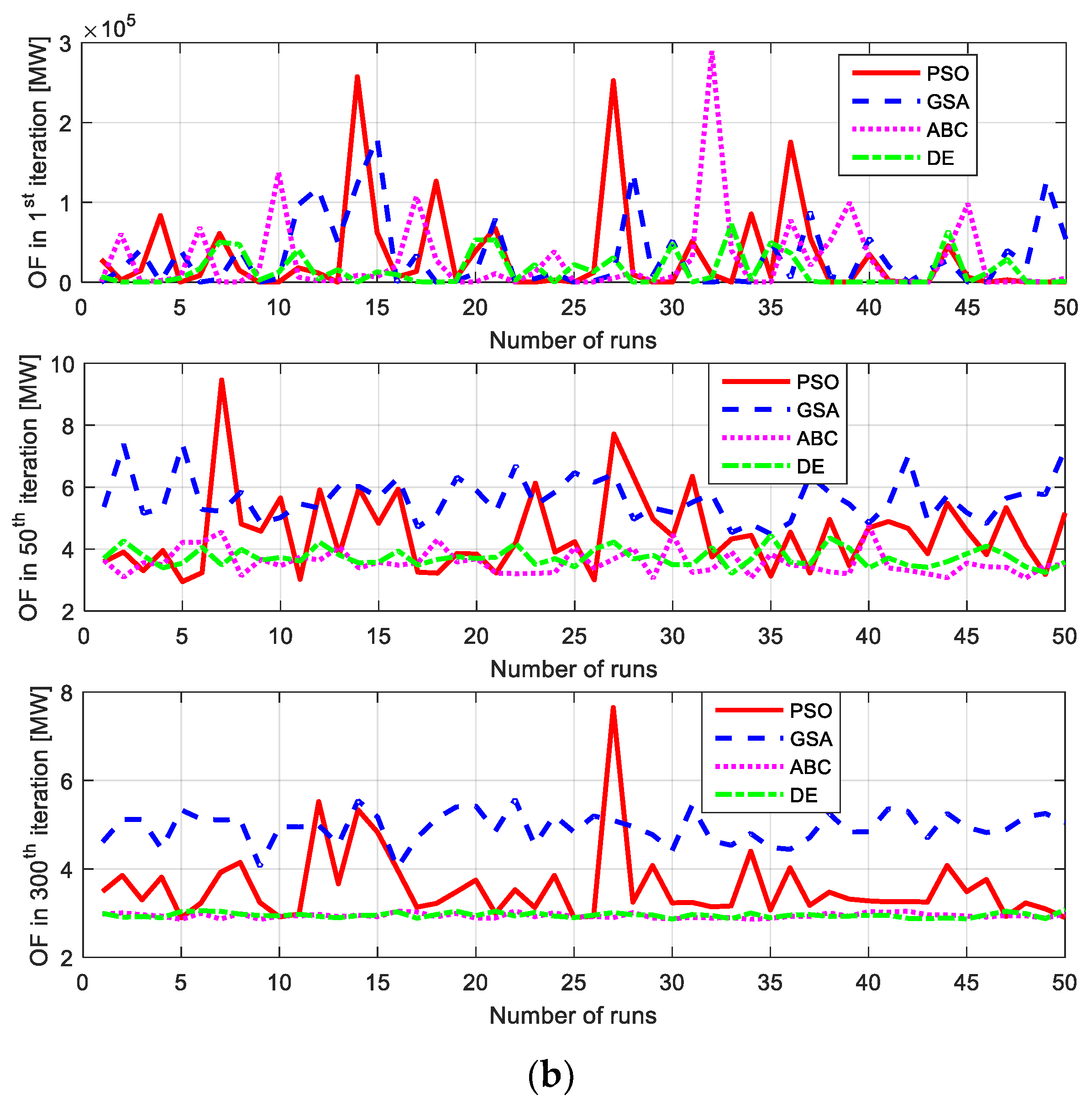
- The comparison of four metaheuristic algorithms applied to single-objective optimal power flow (with the objective function of minimization of power system losses) is presented and tested on both IEEE 9 and IEEE 30 test bus systems and comparison is made with similar studies in the literature;
- -
- The comparison of minimum power system losses obtained using a CONOPT solver and the metaheuristics algorithms is presented;
- -
- The impact of SVC location on power system losses is analyzed in both IEEE 9 and IEEE 30 test bus systems;
- -
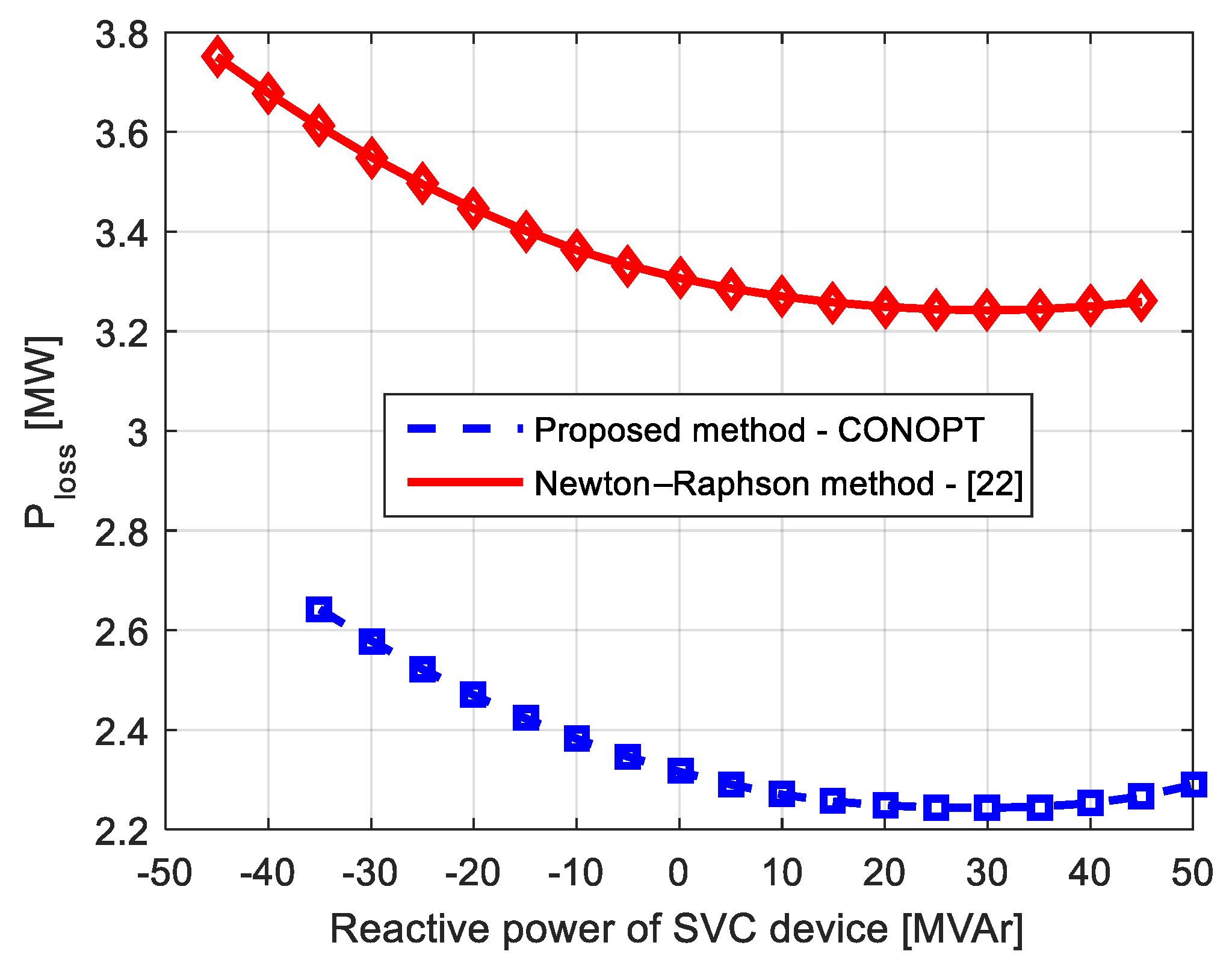
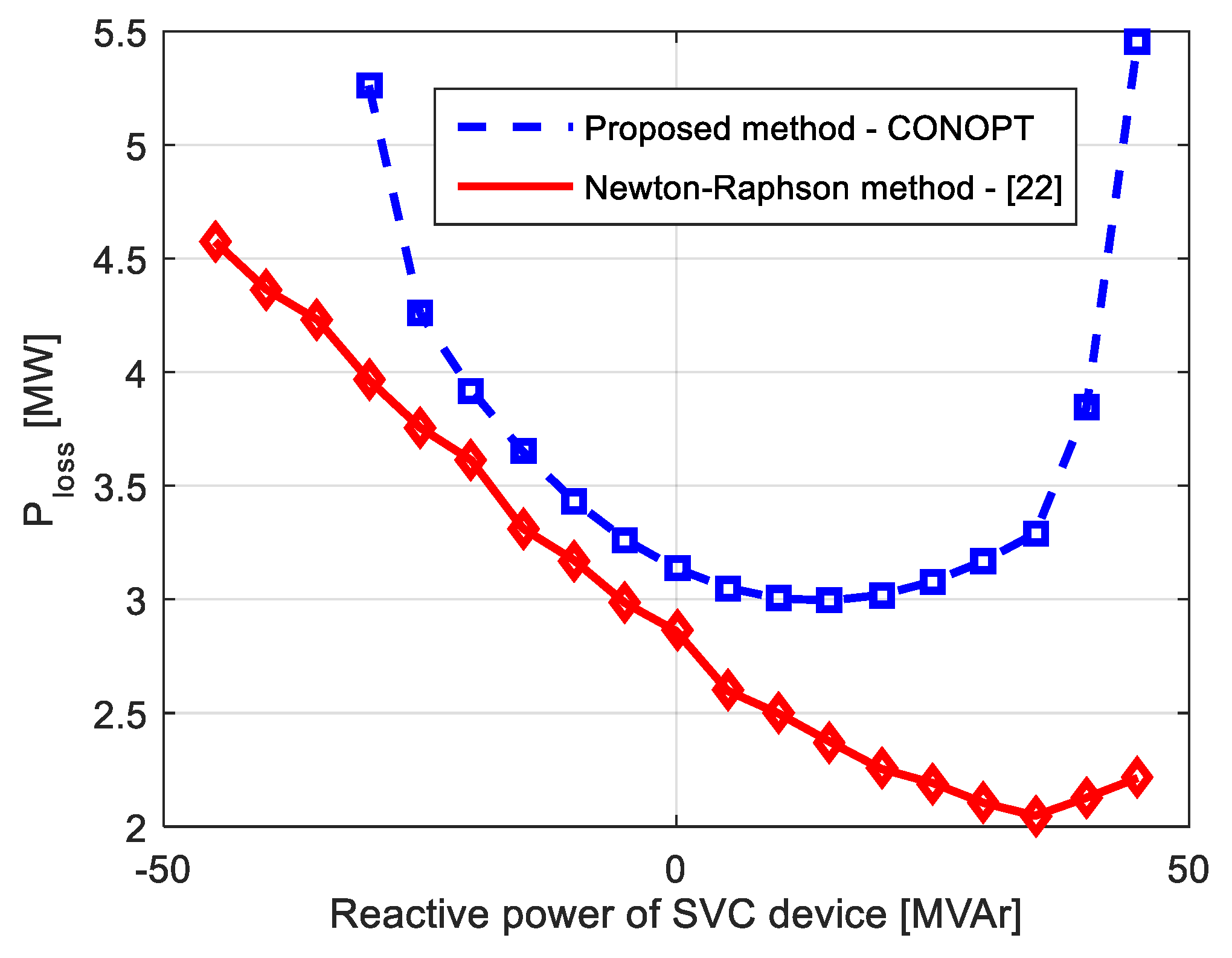
- The impact of the limited reactive power of SVC devices on power system losses is also analyzed in the same test systems;
- -
- The impact of SVC location on power system losses in power networks with renewables is analyzed;
- -
- The impact of different wind power generator connections in power networks on the SVC location is tested;
- -
- For constant load data, the results obtained using the Newton–Rapson method for optimal SVC location and the minimal value of power losses are compared with known solutions from the literature
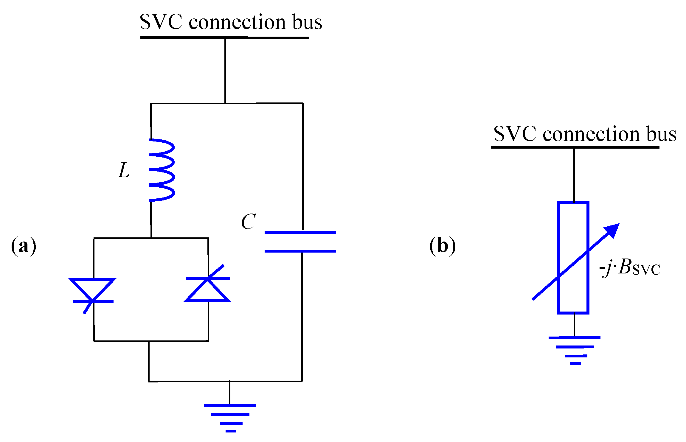
2. SVC Devices
3. Optimal Power Flow Formulation
- -
- Generator constraints:
- -
- Transformer constraints:
- -
- Security constraints:
- -
- Minimization of total fuel cost:where ai, bi, and ci are the cost coefficients of generator i.
- -
- Minimization of total emission:where , , , , and are the emission coefficients of unit i
- -
- Voltage deviation minimization:
- -
- Total active power loss minimization:In an OPF problem, one (single-objective OPF) or more (multi-objective OPF) objective functions can be optimized at the same time.
4. Comparison of Metaheuristics Methods and Solver CONOPT for OPF Problem Solving
4.1. Short Comments on Metaheuristic Methods for OPF
4.2. Basic Information about CONOPT Solver Embedded in GAMS
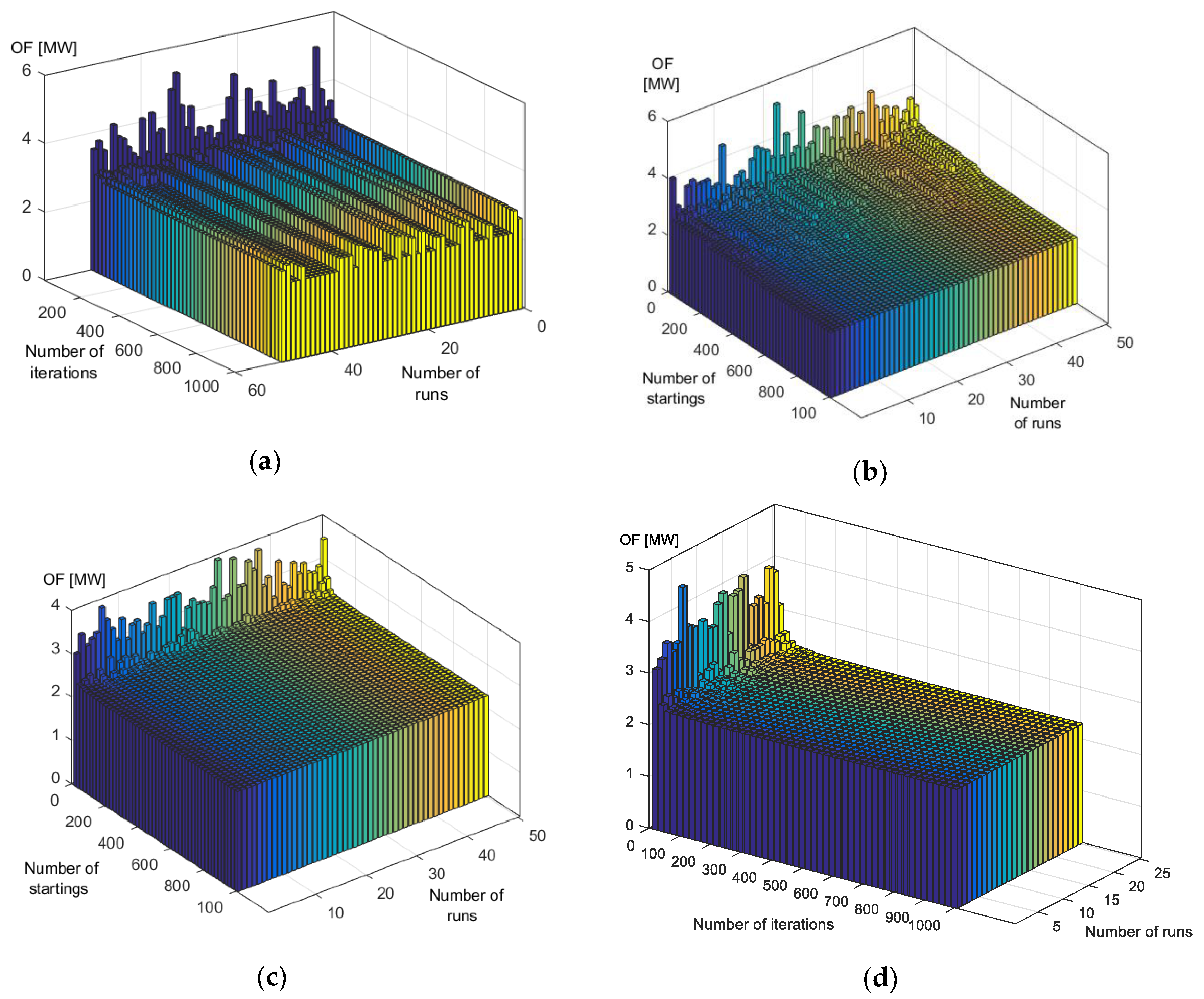
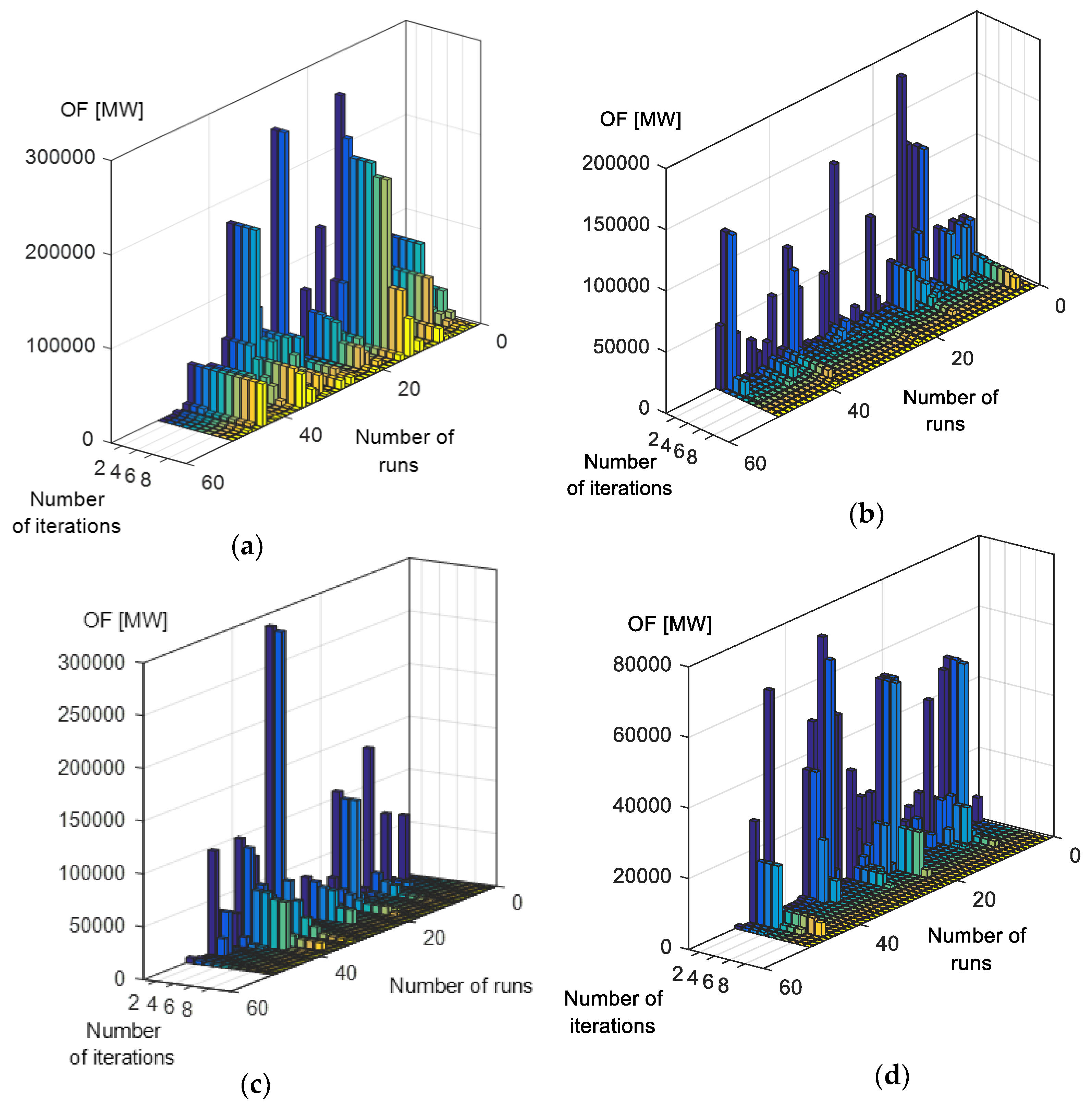
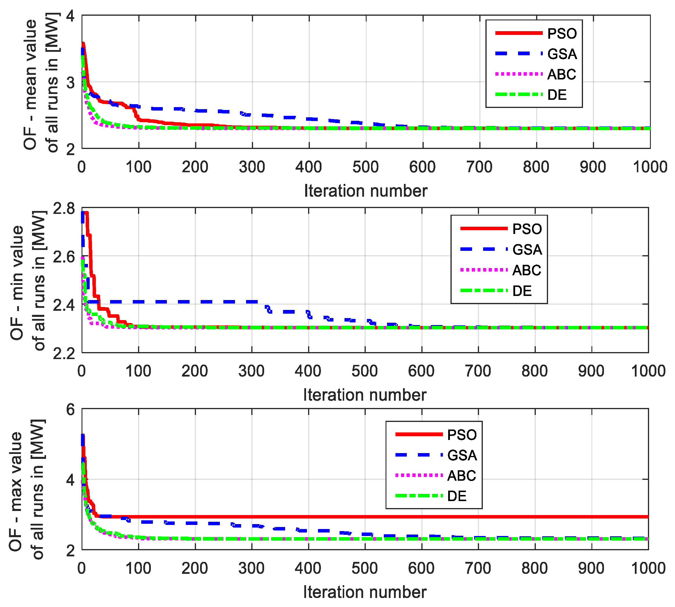
4.3. Results of Comparisons
5. Impact of SVC Location—Simulation Results
- -
- CASE 1—system supply constant load;
- -
- CASE 2—system supply variable load;
- -
- CASE 3—system supply variable load in the presence of a fixed wind generator location; and
- -
- CASE 4—system supply variable load for different wind generator locations.
5.1. CASE 1
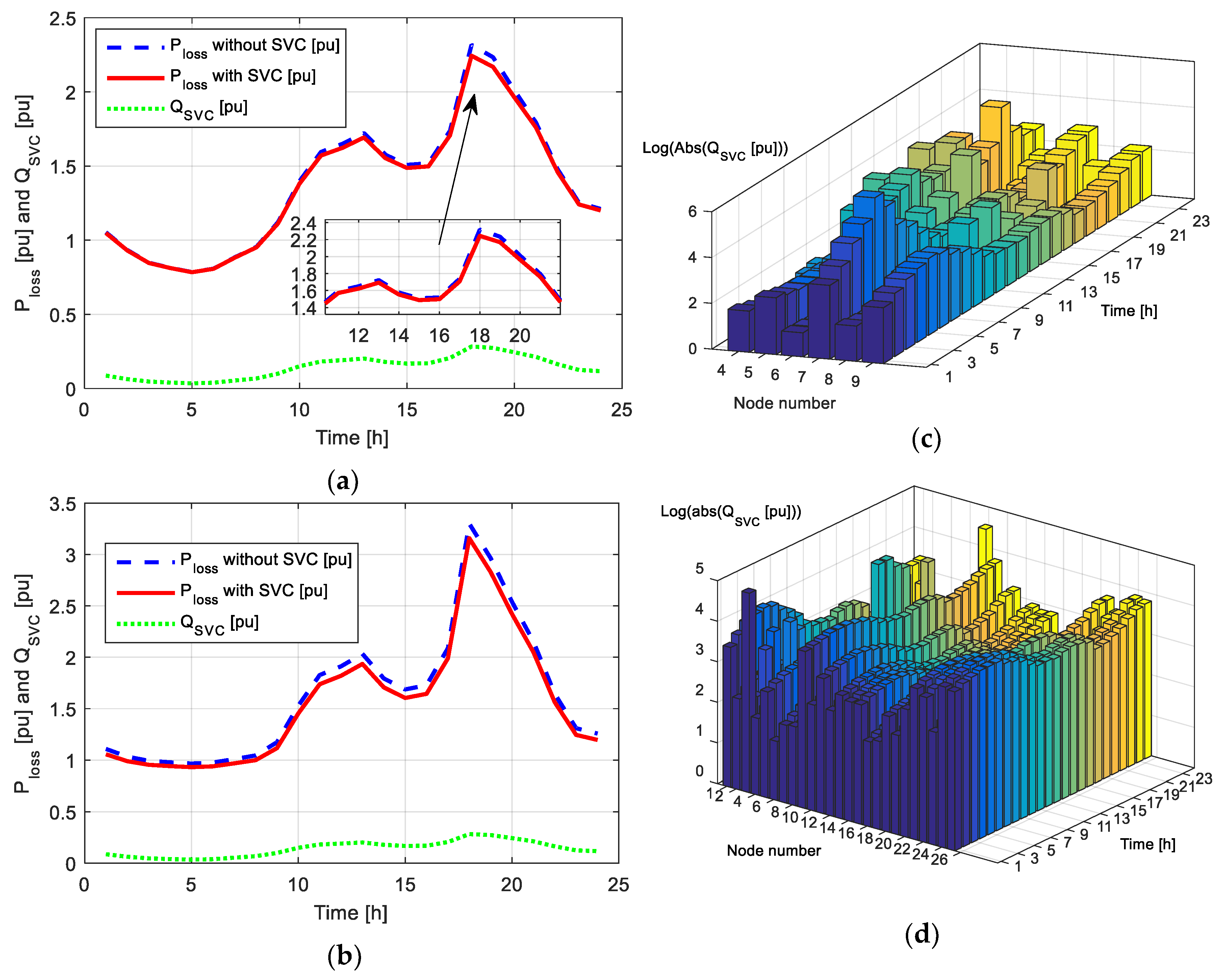
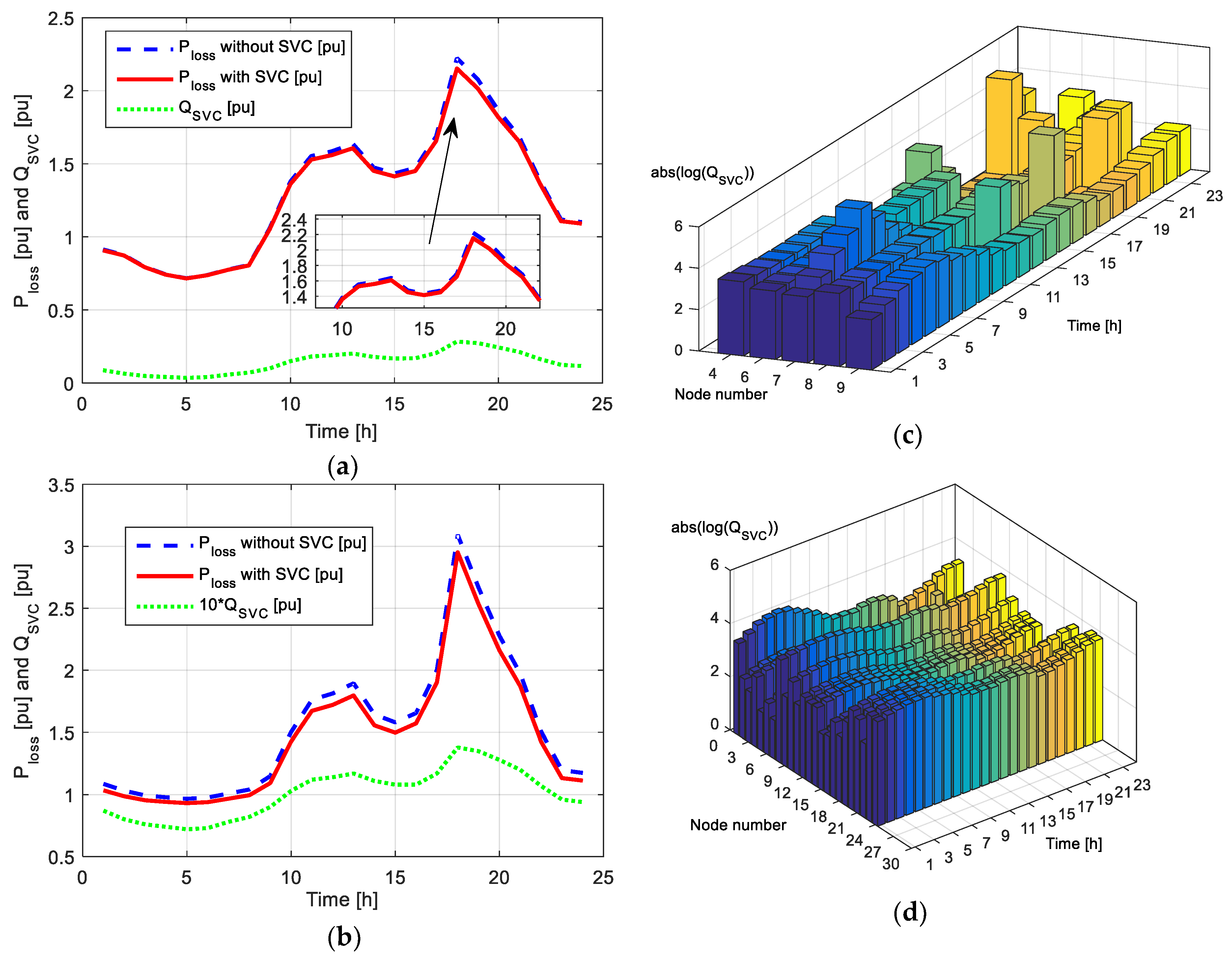
5.2. CASE 2
5.3. CASE 3
5.4. CASE 4
- -
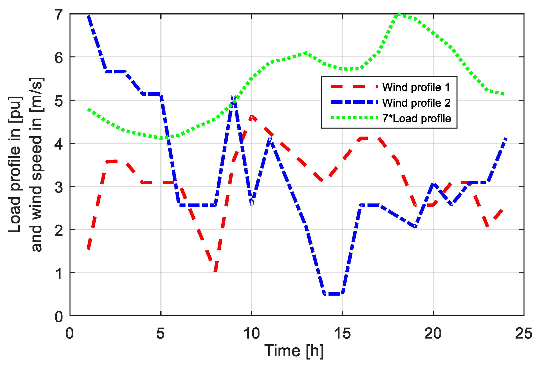
- For both wind profiles, when there are no SVC devices, the optimal location of the wind generator is node 9.
- -
- When the wind generator is connected in nodes 4, 5, 6, 7, or 8 for both wind profiles, the optimal location of SVC device is node 9. When the wind generator is connected in node 9 for both wind profiles, the optimal location of the SVC device is node 5.
- -
- Finally, for wind profile 1, the minimal losses can be obtained if the wind generator is connected in node 5, and SVC in node 9 (25.528 MW). For wind profile 2, the minimal losses can be obtained if the wind generator is connected in node 9, and SVC in node 5 (24.174 MW).
6. Conclusions
Author Contributions
Funding
Conflicts of Interest
References
- Ismael, S.M.; Aleem, S.H.A.; Abdelaziz, A.Y.; Zobaa, A.F. State-of-the-art of hosting capacity in modern power systems with distributed generation. Renew. Energy 2019, 130, 1002–1020. [Google Scholar] [CrossRef]
- Dixon, J.; Moran, L.; Rodriguez, J.; Domke, R. Reactive Power Compensation Technologies: State-of-the-Art Review. Proc. IEEE 2005, 93, 2144–2164. [Google Scholar] [CrossRef]
- Nadeem, M.; Imran, K.; Khattak, A.; Ulasyar, A.; Pal, A.; Zeb, M.Z.; Khan, A.N.; Padhee, M. Optimal Placement, Sizing and Coordination of FACTS Devices in Transmission Network Using Whale Optimization Algorithm. Energies 2020, 13, 753. [Google Scholar] [CrossRef] [Green Version]
- Mondal, D.; Chakrabarti, A.; Sengupta, A. Optimal placement and parameter setting of SVC and TCSC using PSO to mitigate small signal stability problem. Int. J. Electr. Power Energy Syst. 2012, 42, 334–340. [Google Scholar] [CrossRef]
- Chang, C.S.; Qizhi, Y. Fuzzy bang–bang control of static VAR compensators for damping system-wide low-frequency oscillations. Electr. Power Syst. Res. 1999, 49, 45–54. [Google Scholar] [CrossRef]
- Hemeida, M.G.; Hegazy, R.; Mohamed, M.H. A comprehensive comparison of STATCOM versus SVC-based fuzzy controller for stability improvement of wind farm connected to multi-machine power system. Electr. Eng. 2017, 99, 1–17. [Google Scholar] [CrossRef]
- Darabian, M.; Jalilvand, A. A power control strategy to improve power system stability in the presence of wind farms using FACTS devices and predictive control. Int. J. Electr. Power Energy Syst. 2017, 85, 50–66. [Google Scholar] [CrossRef]
- Huang, J.S.; Jiang, Z.H.; Negnevitsky, M. Loadability of power systems and optimal SVC placement. Int. J. Electr. Power Energy Syst. 2013, 45, 167–174. [Google Scholar] [CrossRef]
- Ghahremani, E.; Kamwa, I. Optimal placement of multiple-type FACTS devices to maximize power system loadability using a generic graphical user interface. IEEE Trans. Power Syst. 2013, 28, 764–778. [Google Scholar] [CrossRef]
- Gerbex, S.; Cherkaoui, R.; Germond, A.J. Optimal location of multi-type FACTS devices in a power system by means of genetic algorithms. IEEE Trans. Power Syst. 2001, 16, 537–544. [Google Scholar] [CrossRef]
- Basiri-Kejani, M.; Gholipour, E. Two-level procedure based on HICAGA to determine optimal number, locations and operating points of SVCs in Isfahan–Khuzestan power system to maximise loadability and minimise losses, TVD and SVC installation cost. IET Gener. Transm. Distrib. 2016, 10, 4158–4168. [Google Scholar] [CrossRef]
- Raj, S.; Bhattacharyya, B. Optimal placement of TCSC and SVC for reactive power planning using Whale optimization algorithm. Swarm Evol. Comput. 2018, 40, 131–143. [Google Scholar] [CrossRef]
- Mahdad, B.; Srairi, K. Adaptive differential search algorithm for optimal location of distributed generation in the presence of SVC for power loss reduction in distribution system. Int. J. Eng. Sci. Technol. 2016, 19, 1266–1282. [Google Scholar] [CrossRef] [Green Version]
- Belati, E.A.; Nascimento, C.F.; de Faria, H.; Watanabe, E.H.; Padilha-Feltrin, A. Allocation of Static Var Compensator in Electric Power Systems Considering Different Load Levels. J. Control Autom Electr. Syst. 2019, 30, 1–8. [Google Scholar] [CrossRef]
- Savić, A.; Djurišić, Ž. Optimal sizing and location of SVC devices for improvement of voltage profile in distribution network with dispersed photovoltaic and wind power plants. Appl. Energy 2014, 134, 114–124. [Google Scholar] [CrossRef]
- Xu, X.; Xu, Z.; Lyu, X.; Li, J. Optimal SVC placement for Maximizing Photovoltaic Hosting Capacity in Distribution Network. IFAC-Pap. Online 2018, 51, 356–361. [Google Scholar] [CrossRef]
- Elmitwally, A.; Eladl, A. Planning of multi-type FACTS devices in restructured power systems with wind generation. Int. J. Electr. Power Energy Syst. 2016, 77, 33–42. [Google Scholar] [CrossRef]
- Duan, C.; Fang, W.; Jiang, L.; Niu, S. FACTS Devices Allocation via Sparse Optimization. IEEE Trans. Power Syst. 2016, 31, 1308–1319. [Google Scholar] [CrossRef] [Green Version]
- Benabid, R.; Boudour, M.; Abido, M.A. Optimal location and setting of SVC and TCSC devices using non-dominated sorting particle swarm optimization. Electr. Power Syst. Res. 2009, 79, 1668–1677. [Google Scholar] [CrossRef]
- Jordehi, A.R. Brainstorm optimisation algorithm (BSOA): An efficient algorithm for finding optimal location and setting of FACTS devices in electric power systems. Int. J. Electr. Power Energy Syst. 2015, 69, 48–57. [Google Scholar] [CrossRef]
- Ahmad, A.A.; Sirjani, R. Optimal placement and sizing of multi-type FACTS devices in power systems using metaheuristic optimisation techniques: An updated review. Ain Shams Eng. J. 2019, in press. [Google Scholar] [CrossRef]
- Singh, B.; Agrawal, G. Enhancement of voltage profile by incorporation of SVC in power system networks by using optimal load flow method in MATLAB/Simulink environments. Energy Rep. 2018, 4, 418–434. [Google Scholar] [CrossRef]
- Sebaa, K.; Bouhedda, M.; Tlemcani, A.; Henini, N. Location and tuning of TCPSTs and SVCs based on optimal power flow and an improved cross-entropy approach. Int. J. Electr. Power Energy Syst. 2014, 54, 536–545. [Google Scholar] [CrossRef]
- Subasri, C.K.; Charles Raja, S.; Venkatesh, P. Power quality improvement in a wind farm connected to grid using FACTS device. Power Electron Renew Energy Syst. 2015, 326, 1203–1212. [Google Scholar]
- Liao, H.; Milanović, J. On capability of different FACTS devices to mitigate a range of power quality phenomena. IET Gener. Transm. Distrib. 2017, 11, 2002–2012. [Google Scholar] [CrossRef] [Green Version]
- Ćalasan, M.P.; Nikitović, L.; Mujović, S. CONOPT solver embedded in GAMS for optimal power flow. J. Renew. Sustain. Energy 2019, 11, 046301. [Google Scholar] [CrossRef] [Green Version]
- Warid, W.; Hizam, H.; Mariun, N.; Abdul-Wahab, N.I. Optimal Power Flow Using the Jaya Algorithm. Energies 2016, 9, 678. [Google Scholar] [CrossRef]
- Reddy, S.S.; Panigrahi, B.K. Optimal power flow using clustered adaptive teaching learning-based optimization. Int. J. Bio-Inspired Comput. 2017, 9, 226–234. [Google Scholar] [CrossRef]
- Adaryani, R.; Karami, M.A. Artificial bee colony algorithm for solving multiobjective optimal power flow problem. Int. J. Electr. Power Energy Syst. 2013, 53, 219–230. [Google Scholar] [CrossRef]
- Liang, R.H.; Tsai, S.R.; Chen, Y.T.; Tseng, W.T. Optimal power flow by a fuzzy based hybrid particle swarm optimization approach. Electr Power Syst. Res. 2011, 81, 1466–1474. [Google Scholar] [CrossRef]
- Kecojević, K.; Lukačević, O.; Ćalasan, M. Impact of static var compensator (SVC) devices on power system losses. BH Electr. Eng. 2019, 13, 50–55. [Google Scholar]
- He, L.; Wei, Z.; Yan, H.; Xv, K.Y.; Zhao, M.Y.; Cheng, S. A Day-ahead Scheduling Optimization Model of Multi-Microgrid Considering Interactive Power Control. In Proceedings of the 4th International Conference on Intelligent Green Building and Smart Grid (IGBSG), Yi-chang, China, 6–9 September 2019; pp. 666–669. [Google Scholar]
- Chiu, W.Y.; Sun, H.; Poor, H.V. A Multiobjective Approach to Multimicrogrid System Design. IEEE Trans. Smart Grid 2015, 6, 2263–2272. [Google Scholar] [CrossRef] [Green Version]
- Zheng, X.; Cao, H.; Li, H.; Cui, T.; Jiang, Y.; Zhang, M. Multi-inverters Pre-synchronization VSG Control Strategy for the Microgrid System. In Proceedings of the IEEE 4th International Future Energy Electronics Conference (IFEEC), Singapore, 25–28 November 2019; pp. 1–5. [Google Scholar]
- Mohanty, A.; Viswavandya, M.; Ray, P.K.; Patra, S. Stability analysis and reactive power compensation issue in a microgrid with a DFIG based WECS. Electr. Power Energy Syst. 2014, 62, 753–762. [Google Scholar] [CrossRef]
- Gabbar, H.A.; Abdelsalam, A.A. Microgrid energy management in grid-connected and islanding modes based on SVC. Energy Convers. Manag. 2014, 86, 964–972. [Google Scholar] [CrossRef]
- Abdelsalam, A.A.; Gabbar, H.A.; Sharaf, A.M. Performance enhancement of hybrid AC/DC microgrid based D-FACTS. Int. J. Electr. Power Energy Syst. 2015, 67, 298–323. [Google Scholar] [CrossRef]
- Mithulananthan, N.; Canizares, C.A.; Reeve, J.; Rogers, G.J. Comparison of PSS, SVC, and STATCOM Controllers for Damping Power System Oscillations. IEEE Trans. Power Syst. 2003, 18, 786–792. [Google Scholar] [CrossRef]
- Mithulananthan, N.; Canizares, C.A.; Reeve, J.; Rogers, G.J. New Coordinated Design of SVC and PSS for Multi-machine Power System Using BF-PSO Algorithm. Procedia Technol. 2013, 11, 65–74. [Google Scholar]
- Kundur, P. Power System Stability and Control; McGraw-Hill: Toronto, ON, Canada, 1994. [Google Scholar]
- Benaissa, M.O.; Hadjeri, S.; Zidi, S.A. Impact of PSS and SVC on the Power System Transient Stability. Adv. Sci. Technol. Eng. Syst. 2017, 2, 562–568. [Google Scholar] [CrossRef] [Green Version]
- Yuan, S.Q.; Fang, D.Z. Robust PSS Parameters Design Using a Trajectory Sensitivity Approach. IEEE Trans. Power Syst. 2009, 24, 1011–1018. [Google Scholar] [CrossRef]
- Mutale, J.; Strbac, G. Transmission network reinforcement versus FACTS: An economic assessment. IEEE Trans. Power Syst. 2000, 15, 961–967. [Google Scholar] [CrossRef]
- Lukačević, O.; Ćalasan, M.; Mujović, S. Impact of optimal ESS allocation in IEEE 24-test bus system on total production cost. In Proceedings of the 20th International Symposium POWER ELECTRONICS Ee2019, Novi Sad, Serbia, 23–26 October 2019; pp. 1–5. [Google Scholar]
- Soroudi, A. Power System Optimization Modeling in GAMS; Springer: Basel, Switzerland, 2017. [Google Scholar]
- Duman, S.; Güvenç, U.; Sönmez, Y.; Yörükeren, N. Optimal power flow using gravitational search algorithm. Energy Convers. Manag. 2012, 59, 86–95. [Google Scholar] [CrossRef]
- Bhattacharya, A.; Roy, P.K. Solution of multi-objective optimal power flow using gravitational search algorithm. IET Gener. Transm. Distrib. 2012, 6, 751–763. [Google Scholar] [CrossRef]
- Miranda, V.; Alves, R. Differential Evolutionary Particle Swarm Optimization (DEEPSO): A successful hybrid. In Proceedings of the BRICS Congress on Computational Intelligence & 11th Brazilian Congress on Computational Intelligence, Ipojuca, Brazil, 8–11 September 2019. [Google Scholar]
- Chiu, W.Y. Multiobjective controller design by solving a multiobjective matrix inequality problem. IET Control Theory Appl. 2014, 8, 1656–1665. [Google Scholar] [CrossRef] [Green Version]
- Deng, J.; Mao, Y.; Yang, Y. Distribution Power Loss Reduction of Standalone DC Microgrids Using Adaptive Differential Evolution-Based Control for Distributed Battery Systems. Energies 2020, 13, 2129. [Google Scholar] [CrossRef]
- Ebeed, M.; Kamel, S.; Jurado, F. Chapter 7-Optimal Power Flow Using Recent Optimization Techniques. In Classical and Recent Aspects of Power System Optimization; Elsevier: Amsterdam, The Netherlands, 2018; ISBN 978-0-12-812441-3. [Google Scholar]
- Carpentier, J. Contribution á l’étude du dispatching économique. Bulletin de la Société Française des Électriciens 1962, 8, 431–447. [Google Scholar]
- Frank, S.; Steponavice, I.; Rebennack, S. Optimal power flow: A bibliographic survey I, formulations and deterministic methods. Energy Syst. 2012, 3, 221–258. [Google Scholar] [CrossRef]
- Glover, F. Future paths for integer programming and links to artificial intelligence. Comput. Oper. Res. 1986, 13, 533–549. [Google Scholar] [CrossRef]
- Glover, F.; Kochenberger, G.A. Handbook of Metaheuristic; Springer-International Series in Operations Research & Management Science: New York; Kluwer: Philadelphia, PA, USA, 2003. [Google Scholar]
- Boussaid, I.; Lepagnot, J.; Siarry, P. A survey on optimization metaheuristic. Inf. Sci. 2013, 237, 82–117. [Google Scholar] [CrossRef]
- Radosavljević, J. Metaheuristic Optimization in Power Engineering; IET: London, UK, 2018. [Google Scholar]
- Frank, S.; Steponavice, I.; Rebennack, S. Optimal power flow: A bibliographic survey II, Non-deterministic and hybrid methods. Energy Syst. 2012, 3, 259–289. [Google Scholar] [CrossRef]
- Buch, H.; Trivedi, I.N. On the efficiency of the metaheuristics for solving optimal power flow. Neural Comput. Appl. 2019, 31, 5609–5627. [Google Scholar] [CrossRef]
- Narimani, M.R.; Azizipanah-Abarghooee, R.; Zoghdar-Moghadam-Shahrekohne, B.; Gholami, K. A novel approach to multi-objective optimal power flow by a new hybrid optimization algorithm considering generator constraints and multi-fuel type. Energy 2013, 49, 119–136. [Google Scholar] [CrossRef]
- Andrei, N. Continuous Nonlinear Optimization for Engineering Applications in GAMS Technology; Springer International Publishing AG: Cham, Switzerland, 2017. [Google Scholar]
- Sailaja, M.K.; Maheswarapu, S. Enhanced genetic algorithm based computation technique for multi-objective optimal power flow Solution. Int. J. Electri. Power 2010, 32, 736–742. [Google Scholar]
- Abido, M.A.; Al-Ali, N.A. Multi-objective differential evolution for optimal power flow. In Proceedings of the IEEE International Conference on Power Engineering, Energy and Electrical, Drives, 2009 (POWERENG’09), Lisbon, Portugal, 18–20 March 2009; pp. 101–106. [Google Scholar]
- He, X.; Wang, W.; Jiang, J.; Xu, L. An Improved Artificial Bee Colony Algorithm and Its Application to Multi-Objective Optimal Power Flow. Energies 2015, 8, 2412–2437. [Google Scholar] [CrossRef] [Green Version]
- Available online: https://www.windfinder.com/#3/50.2050/18.7646 (accessed on 20 February 2020).


| Best Solution—Ploss [MW] | Iterations | Computation Time [s] | ||||
|---|---|---|---|---|---|---|
| IEEE 9 | IEEE 30 | IEEE 9 | IEEE 30 | IEEE 9 | IEEE 30 | |
| PSO | 2.317 | 3.39 | 440 | 810 | 10.56 | 317.5 |
| GSA | 2.317 | 3.220 | 650 | 700 | 16.89 | 195.5 |
| ABC | 2.317 | 2.995 | 240 | 600 | 12.24 | 420 |
| DE | 2.316 | 2.994 | 320 | 750 | 8.32 | 247.5 |
| CONOPT | 2.3157972 | 2.9937435 | - | - | 0.073 | 0.092 |
| Losses [MW] | ||
|---|---|---|
| Without SVC-a | 2.3157972 | |
| SVC in Node: | Losses [MW] | Optimal Value of SVC Devices—QSVC in [MVAr] |
| 4 | 2.3029 | 31.962 |
| 5 | 2.3082 | 7.811 |
| 6 | 2.3157 | 28.347 |
| 7 | 2.3033 | 16.992 |
| 8 | 2.3157 | 48.066 |
| 9 | 2.2429 | 28.504 |
| Without SVC | 3.1361950 [MW] | |||||||
|---|---|---|---|---|---|---|---|---|
| SVC in Node: | Losses [MW] | QSVC [MVAr] | SVC in Node: | Losses [MW] | QSVC [MVAr] | SVC in Node: | Losses [MW] | QSVC [MVAr] |
| 3 | 3.1283570 | 7.88470 | 15 | 3.0790903 | 12.11422 | 23 | 3.0615291 | 9.28462 |
| 4 | 3.1102065 | 20.22564 | 16 | 3.1164431 | 6.32258 | 24 | 2.9937435 | 13.83753 |
| 6 | 3.0935250 | 30.53385 | 17 | 3.0808191 | 12.75020 | 25 | 3.0782495 | 7.47845 |
| 7 | 3.1051779 | 13.46546 | 18 | 3.0849214 | 7.83266 | 26 | 3.0832614 | 3.83518 |
| 9 | 3.0595039 | 35.83722 | 19 | 3.0753885 | 8.64813 | 27 | 3.1104100 | 7.02192 |
| 10 | 3.0663123 | 23.01893 | 20 | 3.0824500 | 8.70667 | 28 | 3.1103671 | 13.42805 |
| 12 | 3.1361950 | 9.94304 | 21 | 3.0117611 | 19.28986 | 29 | 3.1100272 | 3.54662 |
| 14 | 3.1270511 | 3.33737 | 22 | 3.0215217 | 18.06944 | 30 | 3.1036651 | 3.66248 |
| QSVCmax = 10 [MVAr] | QSVCmax = 15 [MVAr] | QSVCmax = 20 [MVAr] | ||||
| SVC in Node: | Losses [MW] | Optimal Value of QSVC in [MVAr] | Losses [MW] | Optimal Value of QSVC in [MVAr] | Losses [MW] | Optimal Value of QSVC in [MVAr] |
| 4 | 2.3029 | 8.6 | 2.3029 | 8.6 | 2.3029 | 20.0 |
| 5 | 2.3082 | 7.8 | 2.3082 | 7.8 | 2.3082 | 7.8 |
| 6 | 2.3157 | −4.1 | 2.3157 | −5.5 | 2.3157 | −6.9 |
| 7 | 2.3054 | 10.0 | 2.3035 | 15.0 | 2.3033 | 17.0 |
| 8 | 2.3157 | 10.0 | 2.3157 | 15.0 | 2.3157 | 20.0 |
| 9 | 2.2699 | 10.0 | 2.2562 | 15.0 | 2.2482 | 20.0 |
| QSVCmax = 25 [MVAr] | QSVCmax = 30 [MVAr] | QSVCmax = 35 [MVAr] | ||||
| SVC in Node: | Losses [MW] | Optimal Value of QSVC in [MVAr] | Losses [MW] | Optimal Value of QSVC in [MVAr] | Losses [MW] | Optimal Value of QSVC in [MVAr] |
| 4 | 2.3029 | 25.0 | 2.3029 | 30.0 | 2.3029 | 11.2 |
| 5 | 2.3082 | 7.8 | 2.3082 | 7.8 | 2.3082 | 7.8 |
| 6 | 2.3157 | −8.3 | 2.3157 | −9.7 | 2.3157 | −23.3 |
| 7 | 2.3033 | 17.0 | 2.3033 | 17.0 | 2.3033 | 17.0 |
| 8 | 2.3157 | 25.0 | 2.3157 | 30.0 | 2.3157 | −4.4 |
| 9 | 2.2438 | 25.0 | 2.2429 | 28.5 | 2.2429 | 28.5 |
| QSVCmax = 10 [MVAr] | QSVCmax = 20 [MVAr] | QSVCmax = 30 [MVAr] | ||||
|---|---|---|---|---|---|---|
| SVC in Node: | Losses [MW] | QSVC [MVAr] | SVC in Node: | Losses [MW] | QSVC [MVAr] | SVC in Node: |
| 3 | 3.128 | 7.9 | 3.128 | 7.9 | 3.128 | 7.9 |
| 4 | 3.116 | 10.0 | 3.110 | 20.0 | 3.110 | 20.2 |
| 6 | 3.112 | 10.0 | 3.098 | 20.0 | 3.093 | 30.0 |
| 7 | 3.107 | 10.0 | 1.105 | 13.5 | 3.105 | 13.5 |
| 9 | 3.103 | 10.0 | 3.080 | 20.0 | 3.064 | 30.0 |
| 10 | 3.088 | 10.0 | 3.067 | 20.0 | 3.066 | 23.0 |
| 12 | 3.136 | 10.0 | 3.136 | 14.2 | 3.136 | 30.0 |
| 14 | 3.127 | 3.33 | 3.127 | 3.33 | 3.127 | 3.33 |
| 15 | 3.080 | 10.0 | 3.079 | 12.1 | 3.079 | 12.1 |
| 16 | 3.116 | 6.32 | 3.116 | 6.32 | 3.116 | 6.32 |
| 17 | 3.083 | 10.0 | 3.080 | 12.8 | 3.080 | 12.8 |
| 18 | 3.084 | 7.83 | 3.084 | 7.83 | 3.084 | 7.83 |
| 19 | 3.075 | 8.64 | 3.075 | 8.64 | 3.075 | 8.64 |
| 20 | 3.082 | 8.7 | 3.082 | 8.7 | 3.082 | 8.7 |
| 21 | 3.039 | 10.0 | 3.011 | 19.3 | 3.011 | 19.3 |
| 22 | 3.043 | 10.0 | 3.021 | 18.1 | 3.021 | 18.1 |
| 23 | 3.061 | 9.28 | 3.061 | 9.28 | 3.061 | 9.28 |
| 24 | 3.004 | 10.0 | 2.994 | 13.8 | 2.994 | 13.8 |
| 25 | 3.078 | 7.47 | 3.078 | 7.47 | 3.078 | 7.47 |
| 26 | 3.083 | 3.83 | 3.083 | 3.83 | 3.083 | 3.83 |
| 27 | 3.110 | 7.02 | 3.110 | 7.02 | 3.110 | 7.02 |
| 28 | 3.112 | 10.0 | 3.110 | 13.4 | 3.110 | 13.4 |
| 29 | 3.110 | 3.54 | 3.110 | 3.54 | 3.110 | 3.54 |
| 30 | 3.103 | 3.66 | 3.103 | 3.66 | 3.103 | 3.66 |
| Power Losses [MW] | |
|---|---|
| Without SVC | 33.203 |
| SVC in Node: | Power Losses [MW] |
| 4 | 33.175 |
| 5 | 33.065 |
| 6 | 33.203 |
| 7 | 33.120 |
| 8 | 33.203 |
| 9 | 32.726 |
| Without SVC | 39.048 [MW] | ||||
|---|---|---|---|---|---|
| SVC in Node: | Power Losses [MW] | SVC in Node: | Power Losses [MW] | SVC in Node: | Power Losses [MW] |
| 3 | 38.986 | 14 | 38.926 | 22 | 37.647 |
| 4 | 38.783 | 15 | 38.324 | 23 | 38.097 |
| 5 | 39.048 | 16 | 38.815 | 24 | 37.246 |
| 6 | 38.627 | 17 | 38.409 | 25 | 38.388 |
| 7 | 38.703 | 18 | 38.405 | 26 | 38.393 |
| 9 | 38.238 | 19 | 38.292 | 27 | 38.831 |
| 10 | 38.285 | 20 | 38.397 | 28 | 38.805 |
| 12 | 39.048 | 21 | 37.516 | 29 | 38.774 |
| 30 | 38.693 | ||||
| Power Losses [MW] | |
|---|---|
| Without SVC | 31.102 |
| SVC in Node: | Power Losses [MW] |
| 4 | 31.081 |
| 6 | 31.102 |
| 7 | 31.020 |
| 8 | 31.102 |
| 9 | 30.630 |
| Without SVC | 36.972 [MW] | ||||
|---|---|---|---|---|---|
| SVC in Node: | Power Losses [MW] | SVC in Node: | Power Losses [MW] | SVC in Node: | Power Losses [MW] |
| 3 | 36.911 | 15 | 36.252 | 23 | 36.025 |
| 4 | 36.709 | 16 | 36.741 | 24 | 35.176 |
| 6 | 36.558 | 17 | 36.338 | 25 | 36.315 |
| 7 | 36.634 | 18 | 36.332 | 26 | 36.319 |
| 9 | 36.170 | 19 | 36.219 | 27 | 36.757 |
| 10 | 36.213 | 20 | 36.324 | 28 | 36.732 |
| 12 | 36.972 | 21 | 35.445 | 29 | 36.699 |
| 14 | 36.851 | 22 | 35.576 | 30 | 36.619 |
| Wind Generator in Node 4 | Wind Generator in nOde 5 | Wind Generator in Node 6 | ||||||
| Wind Profile 1 | Wind Profile 2 | Wind Profile 1 | Wind Profile 2 | Wind Profile 1 | Wind Profile 2 | |||
| Without SVC | 33.573 | 33.600 | Without SVC | 25.993 | 25.178 | Without SVC | 33.466 | 34.228 |
| SVC in Node: | Power Losses [MW] | Power Losses [MW] | SVC in Node: | Power Losses [MW] | Power Losses [MW] | SVC in Node: | Power Losses [MW] | Power Losses [MW] |
| 4 | 33.438 | 33.465 | 5 | 25.983 | 25.172 | 4 | 33.440 | 34.202 |
| 6 | 33.573 | 33.600 | 6 | 25.993 | 25.178 | 5 | 33.325 | 34.091 |
| 7 | 33.488 | 33.515 | 7 | 25.908 | 25.093 | 7 | 33.381 | 34.142 |
| 8 | 33.573 | 33.600 | 8 | 25.993 | 25.178 | 8 | 33.466 | 34.228 |
| 9 | 33.107 | 33.133 | 9 | 25.528 | 24.715 | 9 | 32.989 | 33.752 |
| Wind Generator in Node 7 | Wind Generator in Node 8 | Wind Generator in Node 9 | ||||||
| Wind Profile 1 | Wind Profile 2 | Wind Profile 1 | Wind Profile 2 | Wind Profile 1 | Wind Profile 2 | |||
| Without SVC | 29.581 | 29.072 | Without SVC | 33.285 | 33.683 | Without SVC | 25.688 | 24.300 |
| SVC in Node: | Power Losses [MW] | Power Losses [MW] | SVC in Node: | Power Losses [MW] | Power Losses [MW] | SVC in Node: | Power Losses [MW] | Power Losses [MW] |
| 4 | 29.555 | 29.046 | 4 | 33.259 | 33.656 | 4 | 25.680 | 24.297 |
| 5 | 29.443 | 28.934 | 5 | 33.146 | 33.546 | 5 | 25.559 | 24.174 |
| 6 | 29.581 | 29.072 | 6 | 33.285 | 33.683 | 6 | 25.688 | 24.300 |
| 8 | 29.581 | 29.072 | 7 | 33.200 | 33.597 | 7 | 25.603 | 24.215 |
| 9 | 29.104 | 28.595 | 9 | 32.809 | 33.208 | 8 | 25.688 | 24.300 |
| IEEE Test Bus System | Power System with Renewables | Optimization Method | Criteria | |
|---|---|---|---|---|
| Proposed method | 9, 30 | Yes | CONOPT solver | power loss minimization |
| Mondal, 2012 [4] | 14 | Yes | PSO | signal stability problem |
| Huang, 2013 [8] | 30 | No | GA | loadability |
| Basiri-Kejani, 2016 [11] | Isfahan–Khuzestan power system | No | HICAGA | loadability, power system losses, total voltage deviations SVC installation cost |
| Ray, 2018, [12] | 30, 57 | No | WOA, DE, GWO, QODE, QOGWO | voltage collapse proximity indication |
| Mahdad, 2016 [13] | 33, 69 | Yes | DS | power loss minimization |
| Belati, 2019 [14] | 118 | branch and bound algorithm | voltage profile Power loss minimization | |
| Savić, 2014 [15] | distribution network | Yes | GA | Voltage deviations |
| Xu, 2018, [16] | distribution network | Yes | - | Investment cost |
| Benabid, 2009, [19] | 30-bus Algerian 114-bus power system | No | PSO | Voltage stability |
| Singh, 2018 [22] | 9, 30 | No | Newton–Raphson method | Voltage profile Power loss minimization |
© 2020 by the authors. Licensee MDPI, Basel, Switzerland. This article is an open access article distributed under the terms and conditions of the Creative Commons Attribution (CC BY) license (http://creativecommons.org/licenses/by/4.0/).
Share and Cite
Ćalasan, M.; Konjić, T.; Kecojević, K.; Nikitović, L. Optimal Allocation of Static Var Compensators in Electric Power Systems. Energies 2020, 13, 3219. https://doi.org/10.3390/en13123219
Ćalasan M, Konjić T, Kecojević K, Nikitović L. Optimal Allocation of Static Var Compensators in Electric Power Systems. Energies. 2020; 13(12):3219. https://doi.org/10.3390/en13123219
Chicago/Turabian StyleĆalasan, Martin, Tatjana Konjić, Katarina Kecojević, and Lazar Nikitović. 2020. "Optimal Allocation of Static Var Compensators in Electric Power Systems" Energies 13, no. 12: 3219. https://doi.org/10.3390/en13123219
APA StyleĆalasan, M., Konjić, T., Kecojević, K., & Nikitović, L. (2020). Optimal Allocation of Static Var Compensators in Electric Power Systems. Energies, 13(12), 3219. https://doi.org/10.3390/en13123219