Abstract
Growing penetration of uncoordinated Distributed Energy Resources (DERs) in distribution systems is contributing to the increase of the load variability to be covered at the transmission system level. Forced, fast and substantial changes of power plants’ output powers increase the risk of their failures, which threatens the reliable and safe delivery of electricity to end users in the power system. The paper handles this issue with the use of DERs and proposes a bilevel coordination concept of day-ahead operation planning with new kind of bids to be submitted by Distribution System Operators (DSOs) to the Transmission System Operator (TSO). This concept includes the extension of the Unit Commitment problem solved by TSO and a new optimization model to be solved by DSO for planning a smoothed power profile at the Transmission–Distribution (T–D) interface. Both optimization models are described in the paper. As simulations show, the modified 24-h power profiles at T–D interfaces result in a reduction of the demand for operation flexibility at the transmission system level and, importantly, result in a decrease of the number of conventional power plants that are required to operate during a day. Additionally, it has been proved that the modified profiles reduce the congestions in the transmission network. Hence, the concept presented in the paper can be identified as an important step towards the transformation of power systems to low-emission and reliable systems with high share of DERs.
1. Introduction
In the past, the main electricity sources in power systems were thermal power plants. Currently, Distributed Energy Resources (DERs), including Renewable Energy Sources (RESs), arise in distribution systems. However, due to small rated output powers of DERs, their operation has not been coordinated so far. As a result, output powers of wind turbines and photovoltaics (PVs), which play a dominant role in this transformation [1], fluctuate in accordance with the variability of local weather-dependent conditions, and other DERs, like energy storage systems or biogas-fired turbines, operate in a way maximizing independently their own financial profits. Such operation of DERs without regard to the their impact on power system operation, called the ‘produce-and-forget’ approach [2], has consequences if their share becomes significant. Among others, the residual load, which is understood as total electric power consumption minus output powers of all DERs in the power system, is then characterized by larger differences between maximum and minimum values during a day, more frequent and sharp changes in time and less repeatability of the profile shape day after day.
The high variability of the residual load requires a great flexibility in power system. If hydro or pumped-storage power plants are available, they are elastic enough to operate in such conditions [3]. In another case, existing thermal power plants are forced to fluctuate intensively their output powers, and available interconnections with other transmission systems are exploited as much as possible to smooth the variable residual load profile. Since existing thermal power plants are mostly inelastic in operation [2], it requires many start-ups and ramping from them, which implies intensified thermal and pressure stresses in their steam components [4]. When they operate permanently in such conditions, they are at a higher risk of a failure [5], which may result in emergencies in the power system and disruptions of the electricity delivery to end users. Taking into account the EU target for a 32% share of renewable energy in 2030 [6] and discussions about higher targets for further years [7], it becomes essential to find a solution to the problem of how to manage the variability of the residual load, to be covered by conventional power plants, in a reliable and efficient way in power system with a high share of DERs. This issue is handled in this paper.
Investments in power systems are commonly considered as the basic approach to the issue raised above. However, modifications to the design of the existing thermal power plants [4] or their replacement for new ones that are originally flexible enough, e.g., like gas-fired turbines, are expensive and translate into higher generation prices and, therefore, higher electricity bills for end users. Additionally, modern power systems are expected to follow a path where the worn conventional fossil-fueled power plants are replaced, as far as possible, by renewable energy sources [8]. Another investment idea is to place energy storage systems at the transmission system and manage them to smooth the residual load profile, as it is discussed, e.g., in [6,7,8]. However, it has to be highlighted that this solution requires energy storage systems with relatively large storage capacities, which currently can be ensured only by pumped-storage power plants [9]. Their capabilities, in turn, are hardly limited by local geographical conditions.
Undoubtedly, the increasing share of DERs implies investments in network and flexible resources as well as other modernizations in power systems. However, the need for them can be reduced and the problem of residual load variability can be alleviated if an appropriate and comprehensive management system of available resources is applied. It involves the use of not only conventional power plants but also DERs as active participants in the management of the load-generation balance. In this context, four main areas of such a management system can be distinguished as key to managing effectively the residual load variability:
- Close cooperation between Transmission System Operator (TSO) and Distribution System Operators (DSOs);
- Dealing with the fluctuations coming from weather-dependent renewable generation;
- Coordinated planning and real-time management of the operation of various resources across transmission and distribution systems for achieving joint targets;
- Dealing with the uncertainty coming from predictions of weather-dependent renewable generation and load.
In the following paragraphs, the above issues are thoroughly reviewed. The focus is placed on the maturity of the proposed methods and the possibility to use them in the effective and reliable management of the residual load variability in the power system with a high share of DERs.
In terms of the DSO–TSO cooperation, EU legal acts [9,10,11] confirm the growing need for that. The association representing Several European DSOs and the European Network of Transmission System Operators for Electricity (ENTSO-E) wrote together a report in April 2019 where they outlined the framework of such a cooperation [12]. The very comprehensive review on various aspects concerning DSO–TSO cooperation is done in [13]. Among different issues explored there, the missing elements for ensuring such a cooperation are highlighted and discussed there. The highlighted elements involve the need for the coordinated optimization of the operation plan between transmission and distribution systems as well as the need for a market model for flexibility procurement and activation. Basic market models for flexible services from DERs, including the issue of ordering positions of TSO and DSOs in services’ procurement, are considered in [14,15]. Five main possible schemes of cooperation and coordination between DSOs and TSO, including various market models for services from DERs, are drafted in [16]. Among them, the shared balancing responsibility model attracts the attention because it presents a scheme of balancing the distribution system in accordance with a prior schedule agreed between TSO and DSO. This model is also discussed in the ETIP SNET white paper [17], which describes different holistic architectures for future power systems. Among those architectures, there is also a vision of a future power system, which is based on the ‘LINK-paradigm’. In the approach, the power exchanges between directly connected transmission and distribution systems (considered as grid–link components) are scheduled by their operators. A similar model, called ‘model of scheduled program at HV/MV interface’, is drafted in [18]. In paper [19], this approach is discussed as the decentralized optimization in which DSOs submit bids to TSO, and capabilities of DERs are aggregated to bids at the transmission–distribution interface substations. However, as authors of [13] rightly note, all these cooperation schemes and market models proposed so far are still at a very conceptual level. Additionally, there are few simulations in papers, which verify the potential impact of these cooperation schemes on the power system operation. Three basic schemes for activating reserves in DERs are simulated in a game-theoretic way in [20]. A coordinated economic dispatch of TSO and DSO together with the proposition of generalized bid function to approximate the dispatch cost of the distribution system is defined and simulated in [21]. Nonetheless, in both references the simulations are conducted for a single moment, neglecting the impact of DERs’ dispatch levels on time t on their dispatch capabilities on time t + 1.
Another major issue concerning the reliable management of the residual load variability is a method of dealing with the fluctuations coming from weather-dependent renewable generation. Lots of papers are focusing primarily on dealing with the sharp PV output fluctuations caused by cloud passing. To smooth that, modified Maximum Power Point Tracking (MPPT) algorithms for PV controllers are proposed in studies [22,23,24]. However, the trend dominating in the literature is to employ energy storage systems to reduce the PV fluctuations. For example, control strategies using energy storage devices and based on ramp limiting are developed in [25,26,27,28,29] and summarized in [30]. A control method including the use of the fast Fourier signal transformation to generate a reference curve for energy storage systems is presented in [31]. Other studies like [32,33] present methods based on low- and high-pass filters that assign low-frequency fluctuations to be met by the conventional generation and higher frequency fluctuations to be met by local energy storages systems. Accordingly, Simple Moving Average (SMA) strategies, considered as low-pass filters for smoothing the fluctuating generation, are presented in [34,35,36]. SMA strategy converted into the central moving average strategy is shown in [37] and in [38] where additionally fuzzy logic control is applied for supporting the reduction of fluctuations. Battery management fuzzy control for smoothing is also employed in [39]. Another variation of low-pass filters is the non-causal moving average filter, which is considered in [40]. Unlike the referred moving average methods, which belong to linear solutions, a nonlinear programming method for utilizing energy storage system in smoothing the fluctuations is proposed in [41] where minimization of the residual load deviation from a straight line is done by a quadratic equation. A method for smoothing the fluctuations in peak hours with the use non-linear weighting factors is proposed in [42]. Finally, the control of an energy storage system with the combination of real-time dispatch, quasi real-time dispatch and rolling dispatch for minimizing the fluctuations of active power, also with the use of quadratic equations, is presented in [43].
The alternative approach to smoothing the fluctuations in a power system is to control dispatchable power consumption because it also impacts the residual load variability. A method using a demand response of a large number of residential appliances for smoothing the residual load profile is proposed in [44] with the use of Lyapunov optimization for real-time demand scheduling. In the context of dispatching work load in a distributed computing system, the method proposed in [45] includes a sequential two-step process. The first step consists of specifying the dispatch of Uninterruptible Power Source (UPS) batteries with regard to forecasts of renewable generation, whereas the second step realizes the dispatch of deferrable workload on servers in response to random requests from users. In the referred paper, the method for UPS dispatching is based on a quadratic objective function, which is applied to minimize deviations from the expected average load.
It is worth to note, however, that all the above-referred methods deal with the variability through controlling separately PV, energy storage systems or controllable loads, whereas a comprehensive and joint coordination of different DERs with power plants is neglected there. Additionally, the above-referred methods operate mainly in a horizon close to real-time, neglecting the importance of prior scheduling of the power system operation and its contribution to reliable and efficient operation in real-time, also in the context of dealing with the fluctuations. The review in [46] indicates that there is a quite high interest in prior scheduling the operation of DERs, e.g., in a day-ahead horizon, but only with the objective of maximizing revenues or minimizing costs and if they are aggregated to virtual power plants or microgrids. For example, a continuous-time unit commitment model for day-ahead planning is developed in [47], however, representing an extension of the classical unit commitment problem only by additionally dispatching of aggregated loads, and therefore, neglecting other types of DERs. There are also methods, as proposed in studies [48,49,50], which coordinate operation plans of DERs and are based on optimization models with ramp restrictions on the residual load profile. However, making the problem fully linear as it is shown in these studies, with system costs to be minimized, causes the risk of occurring changes in the obtained residual load profile, which are close to imposed ramp limits. As a consequence, it can result in passing from maximum possible ramping-up to maximum possible ramping-down, or vice-versa, and sharp changes appearing then in the residual load profile. This effect is especially visible in figures presented in [50] where DERs are aggregated to a flexible virtual power plant. The little interest in developing the methods for comprehensive planning of DERs’ operation is a gap because, according to the author, a planning method can complement a real-time management method, giving jointly the most attractive results in reducing the residual load variability.
Planning of the power system operation with a significant share of DERs, including weather-dependent generation from the wind and sun, brings the concern about the uncertainty associated with the prediction errors of their generation. It is also an important issue while considering the effective and reliable management of the residual load variability. Study [51] compares and validated six methods (the grey-box model, neural network, quantile random forest, k-nearest neighbors, support vector regression and ensemble averaging) in application to day-ahead forecasting of PV generation, indicating that the clear sky index influences mostly the accuracy of any PV prediction. For wind and solar power forecasting, ensemble methods combining the forecasts from various algorithms are reviewed in [52], whereas application of forecasting methods to load prediction in smart grids is reviewed thoroughly in [53]. However, in spite of all these computationally intelligent load forecasting methods and advances in enhancing their accuracy, there are still prediction errors that have to be managed. Thus, the uncertainty of input data in scheduling problems is often addressed by stochastic or robust optimization. In the case of stochastic scheduling of the power system operation, the forecasted renewable generation is expressed by the Probability Distribution Function (PDF), which is based on numerous historical data. Due to a larger problem size, the computation effort is larger than in the case of deterministic optimization where all input data are known exactly. A thorough review on recent advances in the stochastic optimization in renewable energy applications is presented in [54]. The referred paper includes the comparison of the two-stage and multi-stage stochastic programming algorithms and overview of the model predictive control. Although there are indications of the needs for further researches (e.g., new techniques for scenario generation), the review indicates that the field of stochastic optimization is quite well addressed. As an alternative approach, robust optimization does not use PDF but requires a set of values or boundaries, which the uncertain input data can take. Importantly, it returns a solution that is feasible for all the variants of uncertainty [55]. This approach is described by less computational effort then the stochastic optimization [56]. Application of robust optimization in scheduling of DERs is considered in [57,58] with quite promising perspectives.
To summarize the above literature review, it has been observed that there is a lack of a comprehensive method providing a coordinated DSO–TSO operation planning of various resources available across transmission and distribution systems for dealing cost-effectively with the variability of the residual load. In order to fill the gap, this paper:
- Proposes a bilevel coordination of day-ahead operation planning of transmission and distribution systems, where TSO has a possibility to select an 24-h power profile at each transmission–distribution (T–D) substation interface to be realized on the next day;
- Presents an optimization model that is used by DSO to form a bid of possible smoothed 24-h power profiles at his T–D interface;
- Presents modifications in the ‘classical’ Unit Commitment (UC) problem, which are needed to serve appropriately the bids submitted by all DSOs;
- Validates the optimization model for shaping a modified 24-h power profile at the T–D interface throughout simulations carried out on a power system model.
The choice of day-ahead horizon results from the fact that it is usually the first time when the detailed 24-h operation plan of the transmission system is developed on the basis of relatively exact projections of load and weather-dependent generation.
Referring to the above reviewed literature, the main contributions of this paper are as follows:
- The proposed DSO–TSO coordination is a developed version of the shared balancing responsibility model [16] and can be easily adopted to the LINK-based holistic architecture of the power system [17]. It deals with the variability of the residual load to be covered by conventional power plants and includes: the cost-effective agreeing the 24-h schedules at T–D interfaces and coordination of operation between different DERs and power plants. So far, all these issues have not been considered together in one concept and in that form as presented here.
- The proposed optimization model includes both a new formulation of the non-cost-oriented quadratic objective function for smoothing the 24-h power profile at the T–D interface and more developed operation models of various DERs. These models involve: time-based dependencies of DERs’ operation (ramp rates, minimum online and offline times and states of the charge of energy storage systems); remuneration of DERs for their involvement in shaping the profile at the T–D interface and limitation of the transfer of the cycling operation (defined as frequent changing of the output power by starting up, shutting down, ramping up and ramping down [59]) from conventional power plants to DERs. So far, such an optimization model has not been proposed in the literature.
The concept presented in this paper concerns radial distribution systems, which are directly connected to the transmission system via single T–D interfaces (e.g., transformer and DC link) and the transmission system, which is managed in accordance with the central dispatch model [60]. DERs considered in the paper include: PV, wind turbines, biofuel-fired electricity sources, energy storage systems and active electricity consumers with the capabilities to reduce temporarily their load. Importantly, this paper focuses on dealing with the variability of the residual load at the transmission system. Handling the congestions in distribution systems is not raised here because it is hard to address exhaustively issues of transmission and distribution systems, together with comprehensive validations, in one paper. However, the study presented in this paper aims to give the justification for further researches on extending the presented method by dealing with distribution system issues.
This paper is organized as follows. Section 2 describes in detail the proposed method including: the framework of bilevel cooperation between transmission and distribution systems for day-ahead operation planning (Section 2.1) and descriptions of two optimization models, which are included in the considered cooperation (Section 2.2). In the first case, it is the optimization model for shaping a 24-h power profile at the T–D interface, whereas in the second case, it is a required extension of the unit commitment model that is solved by TSO to serve the bids from all DSOs. A description of simulations carried out on a power system model and a discussion of the obtained results are presented in Section 3. The conclusions are included in Section 4 and references are put at the end of this paper.
Details on the input data and distribution and transmission system models, which are used in simulations described in Section 3, are included in the Supplementary Material.
2. Methodology
2.1. DSO–TSO Coordination of Day-Ahead Operation Planning
Proposed coordination of day-ahead operation planning of transmission and distribution systems was divided into two sequential steps:
- First step—where day-ahead operation planning of local DERs was executed several times by each DSO in order to create several various and possible 24-h power profiles at its T–D interface for the next day.
- Second step—where day-ahead operation planning of power plants was specified by TSO for the next day (business as usual) but, additionally, there was a selection of 24-h power profiles to be realized at T–D interfaces.
These two steps are visualized in Figure 1.
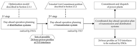
Figure 1.
Bilevel coordination scheme of day-ahead operation planning of transmission and distribution systems.
Usually, the number of DERs in all distribution systems is so very high that including all of them in one central optimization problem would affect too much the computation effort. This issue motivates to aggregate DERs’ capabilities at T–D interfaces as it is considered in [18,19]. This assumption is also adopted in the LINK-based holistic architecture for future power systems [17] where TSO and DERs do not communicate directly to each other but only through DSO and in an aggregated form with a maximally reduced amount of data exchange. It means that single DERs are not visible for TSO, and single resources of the transmission system are not visible for DSO. This paradigm is also adopted in the bilevel coordination scheme presented in this paper.
Representation of DERs’ capabilities in the form of several various profiles for a longer time horizon, as proposed in Figure 1, instead of possible changes per, e.g., each 15 min, has not been considered yet. Obviously, such an approach is attractive as long as capabilities of DERs are properly allocated in such a profile. However, this attractiveness is provided by the optimization model developed in Section 2.2.1.
A detailed description of the two steps presented in Figure 1 is provided in the subsections below.
2.1.1. First Step of the Coordinated Day-Ahead Planning
On day d-1, each DSO collects data for day d from distribution energy resources located in his distribution system. These data are: self-dispatch positions (output powers resulting from earlier concluded bilateral contracts, market contracts or from the priority dispatch), prices declared by DERs’ owners for deviating them from the self-dispatch positions and their technical capabilities/constraints for day d. It is assumed that DERs specify two prices for each market time unit of the next day: one price for upward deviation and the second one for downward deviation. In line with art 53.1 of the EU Electricity Balancing Guideline (EBGL) [60] and art. 8.3 of Regulation (EU) 943/2019 [9] about the imbalance settlement period in scheduling areas, in the proposed method the upward and downward prices are supposed to be declared per each 15 min of day d.
Basing on the data collected from DERs, each DSO specifies a set of several possible 24-h profiles at his T–D interface for the next day, including:
- One non-modified 24-h power profile at T–D interface;
- Several modification/variations of the profile.
The non-modified 24-h profile includes deviations of DERs’ output powers from their self-dispatch positions only due to identified congestions in the distribution network for these positions. The necessary corrections of DERs output powers were introduced on the basis of deviation prices declared by DERs and through minimizing of the total cost, which is to be borne by DSO. However, this 24-h profile had a zero price assigned and was to be seen by TSO.
Modified 24-h profiles at the T–D interface were shaped to deal also with the problems at the transmission system level. In this case, the additional cost of deviating DERs, in relation to the cost of the non-modified profile, poses the price of a modified profile, which is to be seen and to be borne by TSO in the case he chooses that profile for executing on day d. It means that the cost of network congestions, which was calculated for the non-modified profile, was also covered by DSO in the case of any modified profile. It results from the fact that it is the natural cost that should be independent from the TSO decision on choosing a modified or the non-modified profile. This approach is visualized in Figure 2.
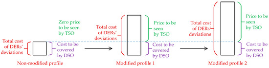
Figure 2.
Visualization of calculating the cost to be covered by the Distribution System Operator (DSO) and the price to be seen by the Transmission System Operator (TSO) for a given modified 24-h power profile.
The process of day-ahead operation planning of a distribution system is visualized in Figure 3.
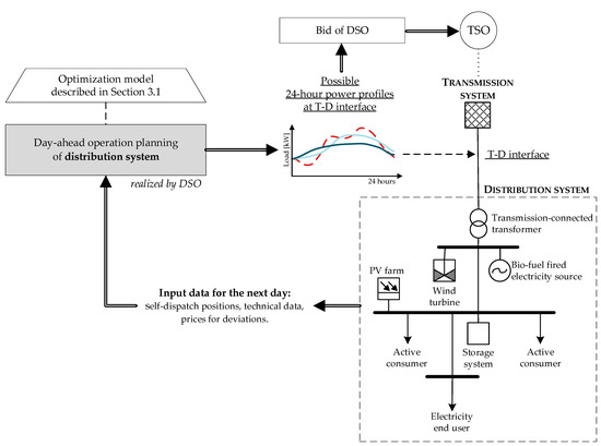
Figure 3.
First step of the coordination—day-ahead operation planning of a distribution system.
A Modified Profile at the T–D Interface
A single modified 24-h profile at the T–D interface was obtained by solving the dedicated optimization model, which dispatches local DERs and makes effort to decrease the variability of the power profile at the T–D interface. In comparison to the non-modified profile, a 24-h power profile obtained from this optimization model had a lower peak value, lower difference between maximum and minimum values, lower power changes between each two consecutive moments and no sharp points. While generating such a modified profile, the optimization model takes many aspects into account, among others, technical constraints of DERs’ operation, remuneration models of DERs, required level of upward and downward power reserved in DERs and network constraints of the distribution system. The mentioned requirement of the powers reserved in DERs results from the following assumptions:
- DSOs are obliged to compensate deviations of real values from their projections if they come from their distribution system and;
- DSOs are obliged to make it possible to offer, e.g., frequency ancillary services by the distributed energy resources.
The mathematical description of the optimization model for generating a modified 24-h power profile at the T–D interface was included in Section 2.2.1.
Design of a DSO Bid
The variety between modified profiles was made via setting gradually a lower limit on the possible total cost of deviations of DERs’ output powers. It is done while launching the optimization model for creating each next modified profile at the T–D interface. Simulations have shown that control of the cost limit impacts most comprehensively the shape of the profile at the T–D interface. The set consisting of one non-modified profile and several modified profiles at the T–D interface poses the bid of DSO for day d, where the design is presented in Figure 4.
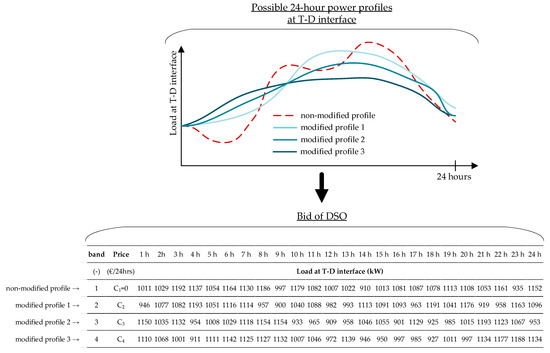
Figure 4.
Design of the bid submitted by DSO to his TSO. For better illustration the 1-h resolution is applied for 24-h profiles, however, actually it should be the 15-min time resolution.
The existence of the non-modified profile in the bid of DSO is obligatory because it allows one to make the day-ahead operation plan of the power system without modification of DERs’ positions if it is justified, e.g., economically. The number of modified profiles in the bid of DSO is a parameter that is to be agreed between all DSOs and TSO. However, in order to form the bid of DSO, the following sequence is applied:
- At first, the non-modified 24-h power profile at the T–D interface is created;
- Then, the first modified profile is created without the limit on the total cost of deviations of the DERs’ output powers. It enables the optimization model to shape the profile as smooth as possible but with the restriction on the total energy transfer to be not higher than the energy in the non-modified profile;
- Finally, other modified profiles are created with the increasingly stringent limits on the total cost per each next profile. These limits were calculated basing on the obtained cost in the first modified profile. The restriction on the total energy transfer was still binding.
2.1.2. Second Step of the Coordinated Day-Ahead Planning
In the second step of the DSO–TSO coordination, bids from power plants and DSOs were collected by TSO to supply the ‘extended’ Unit Commitment (UC) problem. The solution of the extended UC problem is the day-ahead, security-constrained and cost-effective operation plan including:
- Commitment and dispatch of conventional power plants on day d (business as usual);
- 24-h power profiles to be realized at T–D interfaces on day d (novelty).
The extension of the UC problem consists of adding:
- The cost of selected power profiles at T–D interfaces to the minimized objective function;
- Decision variables and equations that allow for selecting which 24-h profile from all submitted by a given DSO in his bid is to be realized during the next day.
In this approach, the modified profiles at T–D interfaces were selected only when it was cheaper than not paying for non-modified profiles but, e.g., with the increased start-ups costs of conventional power plants. A detailed mathematical description of this extension was provided in Section 2.2.2, whereas the process of a day-ahead operation planning of transmission system was visualized below in Figure 5.
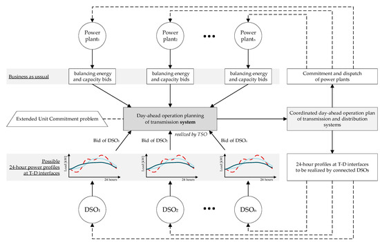
Figure 5.
Second step of the coordination—day-ahead operation planning of the transmission system.
Importantly, taking decisions on power profiles at T–D interfaces in the UC problem is compatible with the assumption of determination of the profile exchange between DSO and TSO in the “Shared Balancing Responsibility model” [16,17].
Although it is out of the scope of this paper, it is worth noting that just after the finished day-ahead operation planning of transmission system, the DSO–TSO coordination of intra-day operation planning should be launched and repeated cyclically with the rolling horizon up to the execution time. It should be done in order to react to new and more exact projections of weather-dependent generation and power consumption, unplanned events in the power system and updates of self-dispatch positions as well as balancing bids. The process of updating cyclically the DSO–TSO operation plan allows for keeping the real power profiles at T–D interfaces as close as possible to the profiles agreed between TSO and DSOs. Additionally, if the prearranged profiles are impossible to be served by TSO or DSOs due to an event happened in the power system (e.g., an emergency in power system) it allows for agreeing new power profiles at the T–D interfaces.
2.2. Optimization Models Included in the DSO–TSO Coordination of Day-Ahead Operation Planning
This section presents mathematical descriptions of two optimization models referred to in the previous section. In the first subsection below, it is the optimization model used by DSO in the first step of the considered DSO–TSO coordination. In the second subsection below, it is the extension of the unit commitment problem used by TSO in the second step of the considered coordination.
2.2.1. Optimization Model for Generating a Modified Profile at the T–D Interface
The mathematical description of the optimization model was put in separate paragraphs concerning the:
- Objective function;
- Power at the T–D interface;
- Technical constraints on the operation of biofuel-fired electricity sources, energy storage systems, PV, wind turbines and active consumers, including limitations of their cycling operation;
- Remuneration models of DERs;
- Cost constraint of the 24-h power profile at the T–D interface;
- Required minimum level of upward and downward power reserved in DERs.
As mentioned in the introduction, this paper describes the concept of DSO–TSO day-ahead operation planning with focus on the variability of the residual load at the transmission system. Due to this reason, congestions at the distribution network and, therefore, power flow calculations were omitted in the mathematical description of the optimization model presented below.
The operation of DERs was modeled by linear equations. It resulted from the fact that, so far, linear expressions modeling the operation of generation units and energy storage systems have been proven to be sufficient [48,50,56,61]. However, it should be noted that the presented constraints concerning the possible operation of DERs are only a proposition of how these sources can be modeled and how their cycling operation can be limited. There are no objections to modeling their operation in a more detailed way or, conversely, to relax their operation constraints.
The issue of uncertainty in renewable generation and load forecasts is addressed by reserving the minimum upward and downward powers in DERs with status “on”. It results from the fact that recent advances in computationally-intelligent forecasting methods reflect quite high accuracy of prediction in the short-time horizon [52,53]. Additionally, the concept presented above assumes the rolling updates of the operation planning process up to the execution time, which gives an ability to compensate day-ahead predictions errors and, therefore, to realize the pre-arranged power profile at the T–D interface.
In the equations below, the unit of power is kW, energy—kWh and time—minutes.
Objective Function
The objective function to be minimized was the sum of squared differences in power at the T–D interface between each two consecutive moments, indexed by , of the next day:
The second element in the objective function, which was the squared difference between the first and last moments of the next day, was included to allow for operating with similar profile shapes day after day. Without that, the optimization model could generate a profile with the broad difference of power between the first and last moments, which prevents from applying similar shapes of the profile at the T–D interface on consecutive days.
As the review presented in the introduction revealed, various objective functions are proposed in the literature to deal with the problem of variable power profile but not one is formulated in the way as presented here. Developing the optimization model with ramp rate limits and the linear cost-oriented objective function, as presented in [50], results in sharp points in the shape of the optimized profile. Although quadratic non-cost-oriented objective functions have been proposed in other papers, they minimize deviations from a reference point. For example, the expected average load is applied as the reference in study [45]. However, it is questionable whether it is always the most appropriate reference point for the whole optimized time horizon (e.g., 24 h). Another study [41] minimizes quadratically the deviations from a straight line, but uses only a battery energy storage system, which neglects the capabilities of other DERs to contribute in the objective function.
The objective function proposed in this paper does not handle any reference point but considers deviations between consecutive time moments as well as possible contribution from various DERs, which is a major novelty.
Power at the T–D Interface
At each moment t, the value of power at the T–D interface was calculated as the difference between loads and generations in the distribution system, e.g., loads of passive end-users , charging powers of energy storage systems , loads of active consumers , generations from bio-fuel-fired electricity sources , generations from PVs and wind sources and discharging powers of energy storage systems . However, the final list of DERs considered in Equation (2) depends on a given distribution system:
Additionally, total electricity transferred under the modified profile was limited by the value of energy transferred under non-modified profile . The included magnitude was the time resolution applied in the optimization model. It is expressed in minutes and was used here for proper calculating of energy (kWh) from power (kW) in time.
Bio-Fuel Fired Electricity Sources
Bio-fuel fired electricity sources were indexed by . Output power can be set between the minimum stable output power and maximum possible output power . Status on/off was modelled by binary variable . Upward and downward power reserves were modelled by and :
Maximum ramping up and down was limited by magnitudes: and which are expressed in kW/min:
Minimum online and offline times ( and ) were introduced to prevent bio-fuel fired electricity sources from too excessive on/off status changes during their scheduling:
PV and Wind Turbines
PV and wind turbines were jointly indexed by . Output power cannot be lower than minimum output power and cannot be higher than projected maximum generation expressed in percent. Magnitude is related to the technical maximum (rated) output power . Status on/off was modeled by binary variable . Upward and downward power reserves were modeled by and :
Maximum ramping up and down is dependent both on the maximum technical capabilities to change output power ) and on the variability of the projected maximum generation at a given time. For example, if is increasing by 10 kW/min, and maximum technical capabilities to decrease the generation is 8 kW/min, this increase can be limited at most to 10 − 8 = 2 kW at this moment:
Energy Storage Systems
Energy storage systems (ESSs) are indexed by . Charging and discharging modes were modeled by binary variables: and . There were minimum and maximum charging and discharging powers: , , , and , which parametrization can be done with a view to limiting the degradation process of the energy storage system (e.g., lower values of charging and discharging powers make thermal conditions better). The state of charge is limited by the maximum and minimum possible states of the charge: and . Apart from using these parameters to specify technical limits of ESSs, they can be also employed to limit the depth of discharge if it impacts the battery lifetime as in the case of, e.g., lead-acid batteries [35]. The round-trip efficiency specifies the ratio of discharged to charged energy. Upward and downward power reserves were modeled by , :
As charging and discharging cycles influence the lifetime of energy storage systems, the parameters and were assumed to limit the numbers of started charging and discharging cycles. In the proposed approach, these magnitudes represent the numbers of charging and discharging cycles resulting from energy contracts (self-dispatch positions) concluded earlier by the ESS owner for the same day. Thus, the ESS life-time was not reduced more when ESS was deviated by DSO from self-dispatch positions. Four binary variables were introduced to model these limitations: indicating the start of charging cycle, indicating the end of a charging cycle and variables and with analogous meanings for discharging cycle:
Active Consumers
Active consumers are indexed by . In this paper, they were modeled as entities that can reduce their load by a fixed value within a fixed duration . The reduction mode is activated by binary variable . Importantly, just after deactivating the reduction mode, which is indicated by , there is a rebound effect. This is a momentary phenomenon when the consumer tries to compensate at least a part of an earlier lost load by an increase in his demand for electric power (e.g., an air-conditioner operates with a higher electricity load in order to restore the most suitable temperature in rooms) [62]. Thus, there is a duration of the rebound effect when the load of an active consumer is higher by the value . In the proposed approach, the value of during time was calculated as the multiplication of: (1) indicating the percent increase on time k after deactivation of the reduction mode and (2) the value of power reduction during the reduction mode.
Maximum number of reduction activations is limited by the magnitude . In order to model that, there are binary variables indicating activation and deactivation of the reduction mode: and .
Additionally, the activation of the reduction mode can be impossible in some periods, e.g., at night from time t1 to time t2.
Minimum Level of Power Reserved in DERs
The sums of upward and downward powers reserved in distributed energy resources cannot be lower than imposed limits: and at each moment:
Remunerations of DERs
For all considered DERs, remuneration models were developed with the use of piece-wise linear functions (special ordered sets), and the only one difference between them was the applied reference point:
- For the energy storage system, it is the state of the charge that results from earlier concluded commercial contracts on purchase and selling energy;
- For other DERs, they are output powers that result from energy market contracts, bilateral contracts or some law regulations (e.g., priority dispatch of RESs).
Due to the reason, the description of remuneration models was narrowed here to the example concerning only energy storage systems.
For each time unit t of the next day, the owner of energy storage system s specifies two unit prices: for deviating up and for deviating down from the state of the charge that results from his prior self-dispatch (the reference point). The remuneration of energy storage system is dependent on the difference between and state of the charge which is a decision variable in the optimization model. This difference is multiplied by if or is multiplied by if , whereas there is no remuneration if . The dependence of on is modeled with three break points. As presented in Figure 6, these break points are at axis Y: , , , and at axis X: , , and . These break points represent incomes for maximum downward deviation, no deviation and maximum upward deviation, respectively (Figure 6). The magnitude is a weighting factor enabling one to specify a for a given . From all three weighting factors (indexed by I = 0, 1, 2) at most two can be nonzero and they must be adjacent in ordering. These assumptions result from the fact that the can be placed either directly between two adjacent breakpoints or exactly on one breakpoint. In the first case, these two breakpoints indicate directly which adjacent weighting factors (respectively to index i) are to be nonzero. In the second case, the one breakpoint indicates exactly one weighting factor (respectively to index i) to adopt the nonzero value. In both cases the sum of all weighting factors has to equal one.
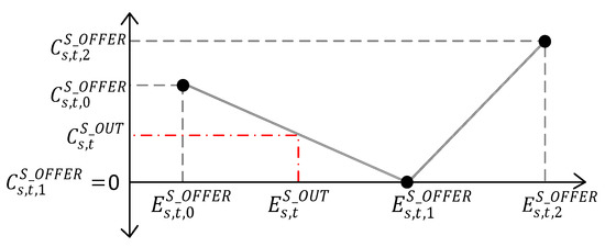
Figure 6.
Visualization of the piece-wise remuneration model of the energy storage system.
Cost of the Modified Profile at the T–D Interface
The cost of a modified 24-h power profile at the T–D interface is the sum of the remunerations of all DERs employed in shaping this profile:
where:
- —the remuneration of energy storage system s at time t;
- —the remuneration of bio-fuel electricity source g at time t;
- —the remuneration of renewable energy source r at time t;
- —the remuneration of active consumer j at time t.
The magnitude can be limited by the arbitrarily set value :
As it is discussed in Section 2.1.1, this constraint is used to make the modified power profiles at the T–D interface different from each other.
2.2.2. Extension of the Unit Commitment Problem
In the optimization model of the classical Unit Commitment (UC) problem, the cost-effective balance between generation and load at the transmission system is achieved by making decisions only on the commitment and dispatch of power plants. In the approach proposed in this paper, the UC problem was extended by the decision on the 24-h power profile at each node representing a connection with a distribution system. This extension is universal and can be introduced regardless of whether it is a network-constrained or security-constrained UC problem.
The first key change in the UC problem is introduced in the equality modeling the balance between generation and load. It consists of the separation of distribution system loads from other loads (e.g., large industrial loads). In the balance equality presented below, distribution systems are indexed by and the load of distribution system d at time t is labeled by :
When the power flows are included and calculated in the UC problem, the formula of the balance equality presented in Equation (50) may be slightly different from that presented here. Load is determined by the multiplication of: (1) binary decision variable indicating which profile (band) b from the bid of DSO d is chosen to be realized and (2) the value of power at time t from a profile included in band b of the bid:
In order to make only one band b chosen for each distribution system d, the following constraint is introduced:
The binary decision variable is also included in the equation, which computes the total costs of all selected profiles at T–D interfaces on the basis of the prices of bands :
Finally, the cost is included in the minimized objective function of the UC problem:
3. Numerical Results and Their Discussion
Simulations were carried out to verify whether the use of the optimization model for shaping the profile at the T–D interface, described in Section 2.2.1, results in:
- A reduction of the demand for operation flexibility at the transmission system level;
- A decrease of the number of conventional power plants that are required to ensure the load-generation balance in the power system during a day;
- An extension of the set of tools that can be used to manage congestions in the transmission network at the stage of operation planning.
The verification procedure was carried out in two steps:
- The 1st step consisted in the generation of several possible 24-h profiles at the T–D interface of a distribution system model. The non-modified 24-h power profile was constructed as the difference between loads and self-dispatched operation of DERs in the distribution system model. Modified power profiles were generated using the optimization model described in Section 2.2.1. Each generated profile posed a separate simulation scenario.
- The 2nd step consisted in the evaluation of the impact of power profiles generated in the 1st step on the transmission system operation. Within a given simulation scenario, a profile obtained in the 1st step was assigned to all load nodes of a transmission system model. The network-constrained UC problem was solved to make it possible to analyze conditions of the transmission system operation.
These two steps are visualized in Figure 7.
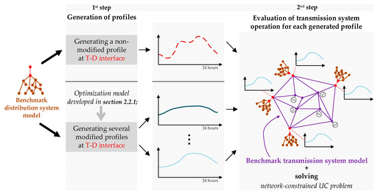
Figure 7.
Two-step procedure of verifying the impact of modified profiles at the T–D interfaces on the day-ahead operation plan and condition of the transmission system operation.
The applied distribution system model was a modified version of the distribution system model developed by the CIGRE Task Force C6.04.02 [63]. There were 8 PV, 1 wind turbine, 2 energy storage systems, 2 biofuel fired electricity sources, 3 active consumers and 10 aggregated passive electricity consumptions. The applied transmission system model was a modified version of the IEEE RTS 24-Bus Transmission System [64]. There were 28 fossil-fueled power plants, 11 load nodes representing connections with distribution systems and 2 large-scale and non-dispatchable renewable energy sources.
The network-constrained UC problem applied in the 2nd step of the verification procedure includes constraints modeling:
- Minimum and maximum output powers of power plants;
- Three temperature-dependent start-up modes of power plants;
- Minimum level of upward and downward power reserved in power plants;
- Maximum upward and downward ramping of output powers of power plants;
- Minimum online and offline times of power plants;
- Minimum number of units operating in each zone of the transmission network;
- Generation and start-up prices of power plants;
- DC power flows and flow limits of the transmission network.
Details on the modifications introduced in the distribution and transmission system models and all input data, which were not originally included in these models, but are required to carry out the simulations, were provided in the Supplementary Material.
Four scenarios were designed to analyze accurately differences in the transmission system operation when non-modified and modified 24-h power profiles were applied to T–D interfaces. In terms of the modified profiles, the scenarios also aimed to highlight the differences when the variety in these profiles was stimulated by changing substantially the limit on the maximum possible cost of DERs’ deviations. The scenarios are as follows:
- Reference scenario R1—represents the following self-dispatch of DERs in the distribution system model: PVs and wind turbines operate with the forecasted weather-dependent generation, bio-fuel fired electricity sources operate with their maximum output powers, active consumers do not activate the reduction mode and energy storage systems realize the arbitrage on an energy market. Therefore, the power profile at the T–D interface was determined as the difference between generations and loads in the distribution system model.
- Main scenario S1—the optimization model developed in Section 2.2.1 was applied. Since the cost of DERs’ deviations was unlimited, the capabilities of DERs were used to the maximum for smoothing 24-h power profile at the T–D interface;
- Main scenario S2—the optimization model developed in Section 2.2.1 was applied. The maximum possible cost of DERs’ deviations was limited to be twice lower than the analogous cost obtained in Scenario S1;
- Main scenario S3—the optimization model developed in Section 2.2.1 was applied. The maximum possible cost DERs’ deviations was limited to be four times lower than the analogous cost obtained in Scenario S1.
Before launching the 2nd step of the verification procedure, all the profiles obtained in the 1st step were respectively scaled up. It was done in a way that:
- In scenario R1 the peak total load in the transmission system model could be met by 80% of total generation capabilities of power plants,
- In scenarios S1, S2 and S3 the total load profile in the transmission system model kept the original proportion to the profile from Scenario R1.
Optimization models used in these simulations were developed in MOSEL programming language, whereas simulations were performed using the Computing & Information Services Center infrastructure at Lodz University of Technology with the use of the FICO Xpress solver. The time resolution was 15 min in the case of generating the power profiles at the T–D interface (1st step of the verification procedure), and 60 min when the UC problem was solved for the transmission system (2nd step of the verification procedure). The obtained simulation results are discussed below.
Figure 8 presents the obtained shapes of the 24-h power profile at the T–D interface in the 1st step of the verification procedure. It can be noted there that the modified profiles S1, S2 and S3 were much more smooth than profile R1, which represents the outcome of the only self-dispatch of DERs. The modified power profiles had no spikes, no sharp changes over time and had lower differences between peak and off-peak powers than the non-modified profile R1. Even the profile S3, where the strongest limit was set on the cost of DERs’ deviations, seems to be more attractive than profile R1. Table 1, Table 2 and Table 3 present the results from solving the network-constrained UC problem for the transmission system model with the adoption of the obtained profiles (the 2nd step of the verification procedure).
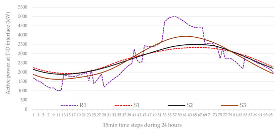
Figure 8.
Shapes of the 24-h power profile at the T–D interface, obtained in scenarios: R1, S1, S2 and S3. Positive values on axis Y mean the transfer of power from transmission system to the distribution system.

Table 1.
The operation condition of power plants.
Table 2.
Peak loads and occurrences of congestions in the transmission network.
Table 3.
Costs of the transmission system operation.
As Table 1 presents, when the 24-h profile obtained in the 1st step of scenario S1 was adopted to load nodes in the transmission system model there were only one hot start-up and one shut-down within 24 h. To compare, in scenario R1, which represents the lack of DERs’ coordination, there were 16 start-ups and shut-downs of power plants within 24 h. In scenarios S2 and S3, which represent modified profiles at the T–D interface with imposed cost limits, there were 3 and 8 of the on/off status changes, respectively, which was still significantly fewer than in scenario R1. In accordance with [5], the operation of thermal power plants without frequent start-ups and shut-downs decreased the risk of their failure, which could be identified as making the power system operation more reliable.
Results from Table 1 also unveiled that in scenarios S1, S2 and S3 there were fewer occurrences of power plants forced to operate with the maximum possible ramping, and more occurrences of their constant output powers within two consecutive moments. It confirms that there was less demand for variable operation of electricity sources in the transmission system when the proposed optimization model for shaping power profiles at T–D interfaces was applied.
Finally, the number of all power plants, which were committed to operate within 24 h, was lower in scenario S1, S2 and S3, but the number of power plants operating then without any break was higher. Therefore, there was a lower need for conventional electricity sources, like fossil-fueled power plants, but these units, which were committed to work, had better operation conditions.
In terms of power flows in scenario S1, S2 or S3, there were fewer moments when the transmission branches were fully loaded. As Table 2 shows, it was associated with lower peak loads at nodes representing connections with distribution systems (T–D interfaces). Importantly, a fully loaded branch indicates that the optimization solver had taken effort to keep the power flow not higher than the power flow limit. It is done to by a reduction of generation from a cheaper unit and replacement of that by a more expensive generation. Hence, the bids of DSOs, together with the extended UC problem as proposed in Section 2.2.2, could extend the set of tools that can be used by TSO to manage congestions in the transmission network at the stage of operation planning.
However, the most important fact was the lower total cost of transmission system operation in scenarios S1, S2 and S3. As Table 3 shows, there were significant reductions of start-up and generation costs of power plants in these scenarios in comparison to scenario R1.
It has to be noted that costs of modified 24-h power profiles at T–D interfaces were not included in the total costs presented in Table 3. On the other hand, the presented results indicate what the maximum additional cost could be incurred for these modified profiles to keep their selection economically attractive when solving the extended UC problem by TSO. As Table 3 shows, in the case of scenario S1, 24-h modified profiles at T–D interfaces were attractive up to €470,182 of their costs in total, which was simultaneously saved in the operation of power plants when comparing to scenario R1. In fact, reflection of ramping costs of power plants in the minimized objective function of the UC problem, as considered, e.g., in [65,66], could result in even more stronger economic justification for utilizing DERs in smoothing the 24-h profiles at T–D interfaces.
The obtained results make the proposed method attractive in the perspective of other methods that focus mainly on the involvement of energy storage systems to alleviate the problem of the residual load variability. Among them, the common approach is to extend the unit commitment problem solved at the transmission system level by dispatching of energy storage systems. As validations in studies [66,67,68,69,70] show, the approach is also reflected in the reduced total costs of the power system operation and in lower numbers of start-ups required from conventional power plants. However, it is worth underlining that it is mostly based on large-scale energy storage systems and rather not easily applicable for much more numerous small-scale energy storage systems and other types of DERs, which an increase is expected in distribution systems. An interesting study and results are shown in [35] where the proposed method controls the renewable generation, energy storage systems and demand side management in a microgrid and is proved to smooth the power exchange with the utility grid. However, this method is dedicated only for real-time controlling. Studies [48,49,50] show optimization models for scheduling the operation of various DERs with the linear cost-oriented objective function and linear constraints on ramping the power exchange with the utility grid. However, it results in sharp points appearing in the profile. As Figure 8 shows, the method proposed in this paper is free from this feature.
The results presented in this section give the sufficient justification and motivation for carrying out further research. These studies are going to extend the presented concept by dealing with congestions in the distribution network. As indicated in Section 2.1.2, there is also a need to develop a DSO–TSO coordination of intra-day operation planning with a rolling horizon up to execution time. On the other hand, it is also crucial to verify whether prices of modified profiles at T–D interfaces, which are identified as attractive in the extended UC problem, after disaggregation, are still attractive to DERs, which make the profiles.
4. Conclusions
The growing share of uncoordinated Distributed Energy Resources (DERs) increases the variability of the load to be covered by conventional power plants. Permanent operation under such conditions makes the power plants more vulnerable to failures. It, in turn, increases the risk of emergencies in the power system and, therefore, poses a major threat to reliable electricity delivery.
This paper shows how to handle this issue at the stage of day-ahead operation planning and proposes a concept of smoothing the power profiles at transmission–distribution (T–D) interfaces by the use of DERs. The concept assumes that each Distribution System Operator (DSO) creates a bid of several possible 24-h smoothed power profiles at its T–D interface for the next day and submits that to his Transmission System Operator (TSO). Subsequently, TSO solves the extended Unit Commitment (UC) problem to specify not only the commitment and dispatch of conventional electricity sources at the transmission system level but also to choose one profile for each T–D interface to be realized on the next day. In order to create a bid, DSO uses a dedicated optimization model for shaping several various and possible 24-h smoothed power profiles at its T–D interface for the next day.
As simulation results show, the proposed optimization model generates a 24-h power profile at the T–D interface, which is more much attractive than the non-modified profile resulting only from the self-dispatch of local DERs. The obtained, modified power profile at the T–D interface has no spikes, no sharp changes over time and has lower differences between peak and off-peak powers than the non-modified profile. Simulations carried out on the transmission system model proved that fewer conventional power plants are required to operate during a day if distribution systems follow modified profiles at their T–D interfaces. Importantly, there are also much fewer start-ups and shut-downs of power plants, and their output powers were less fluctuating in comparison to the scenario where is no coordination of DERs but only their self-dispatch. In terms of power flows, when there were modified 24-h profiles at the T–D interfaces, there were fewer moments when the branches at transmission network were fully loaded. Finally, calculated costs of transmission system operation with and without modified profiles at T–D interfaces indicate that there was a significant economic justification for further developing the solution presented in this paper.
Therefore, it could be concluded that the concept presented in this paper gives a new view on how the transformation to low-emission and reliable power system with a high share of DERs can be supported. It has been proven that this concept brings less need for conventional power plants and gives better operation conditions for those ones that are committed to operate. Importantly, the better operation conditions of power plants prevent them from failures and, as a result, emergencies in the power system. Finally, pre-definition of the profile exchange between DSO and TSO, as presented in this concept, can be considered as contributing to the ‘Shared Balancing Responsibility model’ and as being in line with the ‘LINK-based architecture’ for future power systems.
Supplementary Materials
Details on the modifications introduced in the distribution and transmission system models and all input data which are not originally included in these models, but were required to carry out the simulations, are provided at https://www.mdpi.com/1996-1073/13/14/3559/s1.
Funding
This research received no external funding.
Acknowledgments
The author would like to express the gratitude to the FICO corporation for provision of academic licenses for Xpress Optimization Suite to Institute of Electrical Power Engineering at Lodz University of Technology.
Conflicts of Interest
The author declares no conflict of interest.
References
- REN21. REN21—2019 Global Status Report; REN21: Paris, France, 2019. [Google Scholar]
- Pérez-Arriaga, I.J.; Ruester, S.; Schwenen, S.; Battle, C.; Glachant, J.-M. From Distribution Networks to Smart Distribution Systems: Rethinking the Regulation of European Electricity DSOs; RSCAS—European University Institute: Firenze, Italy, 2013. [Google Scholar]
- Rehman, S.; Al-Hadhrami, L.M.; Alam, M.M. Pumped hydro energy storage system: A technological review. Renew. Sustain. Energy Rev. 2015, 44, 586–598. [Google Scholar] [CrossRef]
- Cochran, J.; Lew, D.; Kumar, N. Flexible Coal Evolution from Baseload to Peaking Plant; NREL: Golden, CO, USA, 2013. [Google Scholar]
- Kumar, N.; Besuner, P.; Lefton, S.; Agan, D.; Hilleman, D. Power Plant Cycling Costs; NREL: Golden, CO, USA, 2012. [Google Scholar]
- EU. European Union Directive (EU) 2018/2001 on the promotion of the use of energy from renewable sources. Off. J. Eur. Union 2018, 2018, 1–128. [Google Scholar]
- Miller, G. Beyond 100% renewable: Policy and practical pathways to 24/7 renewable energy procurement. Electr. J. 2020, 33, 106695. [Google Scholar] [CrossRef]
- Zappa, W.; Junginger, M.; van den Broek, M. Is a 100% renewable European power system feasible by 2050? Appl. Energy 2019, 233–234, 1027–1050. [Google Scholar] [CrossRef]
- European Union Regulation (EU). 2019/943 of 5 June 2019 on the internal market for electricity. Off. J. Eur. Union 2019, 158, 54–124. [Google Scholar]
- European Union Directive (EU). 2019/944 of 5 June 2019 on common rules for the internal market for electricity and amending Directive 2012/27/EU. Off. J. Eur. Union 2019, 158, 125–199. [Google Scholar]
- Comission Regulation (EU). 2017/1485 of 2 August 2017 on electricity transmission system operation. Off. J. Eur. Union 2017, 220, 1–120. [Google Scholar]
- CEDEC; EDSOE; ENTSO-E; EURELECTRIC; GEODE TSO-DSO. Report—An Integrated Approach to Active System Management; CEDEC–ENTSO-E–GEODE–E.DSO–EURELECTRIC: Berlin, Germany, 2019. [Google Scholar]
- Lind, L.; Cossent, R.; Chaves-Ávila, J.P.; Gómez San Román, T. Transmission and distribution coordination in power systems with high shares of distributed energy resources providing balancing and congestion management services. Wiley Interdiscip. Rev. Energy Environ. 2019, 8, 1–19. [Google Scholar] [CrossRef]
- Nieto-martin, J.; Bunn, D.W.; Varga, L. Design of Local Services Markets for Pricing DSO-TSO Procurement Coordination. In Proceedings of the 2018 IEEE Power & Energy Society General Meeting (PESGM), Portland, OR, USA, 5–10 August 2018; pp. 1–5. [Google Scholar]
- Vicente-Pastor, A.; Nieto-Martin, J.; Bunn, D.W.; Laur, A. Evaluation of flexibility markets for retailer-dso-tso coordination. IEEE Trans. Power Syst. 2019, 34, 2003–2012. [Google Scholar] [CrossRef]
- Gerard, H.; Rivero Puente, E.I.; Six, D. Coordination between transmission and distribution system operators in the electricity sector: A conceptual framework. Util. Policy 2018, 50, 40–48. [Google Scholar] [CrossRef]
- ETIP-SNET. White Paper—Holistic Architectures for Future Power Systems; INTENSYS4EU: Brussels, Belgium, 2019. [Google Scholar]
- Delfanti, M.; Galliani, A.; Olivieri, V. The new role of DSOs: Ancillary services from RES towards a local dispatch. CIRED Work. 2014, 1, 1–5. [Google Scholar]
- Kristov, L.; De Martini, P.; Taft, J.D. A tale of two visions: Designing a decentralized transactive electric system. IEEE Power Energy Mag. 2016, 14, 63–69. [Google Scholar] [CrossRef]
- Le Cadre, H.; Mezghani, I.; Papavasiliou, A. A game-theoretic analysis of transmission-distribution system operator coordination. Eur. J. Oper. Res. 2019, 274, 317–339. [Google Scholar] [CrossRef]
- Yuan, Z.; Hesamzadeh, M.R. Hierarchical coordination of TSO-DSO economic dispatch considering large-scale integration of distributed energy resources. Appl. Energy 2017, 195, 600–615. [Google Scholar] [CrossRef]
- Yan, R.; Saha, T.K. Power Ramp Rate Control for Grid Connected Photovoltaic System. In Proceedings of the 9th International Power and Energy Conference (IPEC), Singapore, 27–29 October 2010; pp. 83–88. [Google Scholar]
- Sangwongwanich, A.; Yang, Y.; Blaabjerg, F. A Cost-effEctive Power Ramp-Rate Control Strategy for Single-Phase Two-Stage Grid-Connected Photovoltaic Systems. In Proceedings of the 2016 IEEE Energy Conversion Congress and Exposition (ECCE), Milwaukee, WI, USA, 18–22 September 2016; pp. 1–7. [Google Scholar]
- Chen, X.; Du, Y.; Wen, H. Forecasting Based Power Ramp-Rate Control for PV Systems Without Energy Storage. In Proceedings of the 2017 IEEE 3rd International Future Energy Electronics Conference and ECCE Asia (IFEEC 2017-ECCE Asia), Kaohsiung, Taiwan, 3–7 June 2017; pp. 733–738. [Google Scholar]
- Alam, M.J.E.; Muttaqi, K.M.; Sutanto, D. A novel approach for ramp-rate control of solar PV using energy storage to mitigate output fluctuations caused by cloud passing. IEEE Trans. Energy Convers. 2014, 29, 507–518. [Google Scholar]
- Akagi, S.; Yoshizawa, S.; Ito, M.; Fujimoto, Y.; Miyazaki, T. Electrical Power and Energy Systems Multipurpose control and planning method for battery energy storage systems in distribution network with photovoltaic plant. Electr. Power Energy Syst. 2020, 116, 105485. [Google Scholar] [CrossRef]
- Salehi, V.; Radibratovic, B. Ramp rate control of photovoltaic power plant output using energy storage devices. IEEE Power Energy Soc. Gen. Meet. 2014, 2014, 1–5. [Google Scholar]
- Zhou, H.; Bhattacharya, T.; Tran, D.; Siew, T.S.T.; Khambadkone, A.M. Composite energy storage system involving battery and ultracapacitor with dynamic energy management in microgrid applications. IEEE Trans. Power Electron. 2011, 26, 923–930. [Google Scholar] [CrossRef]
- Zhao, Q.; Xian, L.; Roy, S. Kong xin optimal control of pv ramp rate using multiple energy storage system. Phys. A Stat. Mech. Appl. 2007, 374, 483–490. [Google Scholar]
- Karmiris, G.; Tengnér, T. Control Method Evaluation for Battery Energy Storage System Utilized in Renewable Smoothing. In Proceedings of the IECON 2013—39th Annual Conference of the 2013 IEEE Industrial Electronics Society, Vienna, Austria, 10–13 November 2013; pp. 1566–1570. [Google Scholar]
- Ahmed, M.; Member, S.; Kamalasadan, S.; Member, S. An Approach for Net-Load Management to Reduce Intermittency and Smooth the Power Output on Distribution Feeders with High PV Penetration. In Proceedings of the 2018 IEEE Industry Applications Society Annual Meeting (IAS), Portland, OR, USA, 23–27 September 2018; pp. 1–9. [Google Scholar]
- Kim, S.K.; Jeon, J.H.; Cho, C.H.; Ahn, J.B.; Kwon, S.H. Dynamic modeling and control of a grid-connected hybrid generation system with versatile power transfer. IEEE Trans. Ind. Electron. 2008, 55, 1677–1688. [Google Scholar] [CrossRef]
- Meng, L.; Dragicevic, T.; Guerrero, J. Adaptive Control of Energy Storage Systems for Power Smoothing Applications. In Proceedings of the 2017 IEEE 3rd International Future Energy Electronics Conference and ECCE Asia (IFEEC 2017—ECCE Asia), Kaohsiung, Taiwan, 3–7 June 2017; pp. 1014–1018. [Google Scholar]
- Kakimoto, N.; Satoh, H.; Takayama, S.; Nakamura, K. Ramp-rate control of photovoltaic generator with electric double-layer capacitor. IEEE Trans. Energy Convers. 2009, 24, 465–473. [Google Scholar] [CrossRef]
- Pascual, J.; Sanchis, P.; Marroyo, L. Implementation and control of a residential electrothermal microgrid based on renewable energies, a hybrid storage system and demand side management. Energies 2014, 7, 210–237. [Google Scholar] [CrossRef]
- Hund, T.D.; Gonzalez, S.; Barrett, K. Grid-Tied PV System Energy Smoothing. In Proceedings of the 2010 35th IEEE Photovoltaic Specialists Conference, Honolulu, HI, USA, 20–25 June 2010; pp. 2762–2766. [Google Scholar]
- Pascual, J.; Barricarte, J.; Sanchis, P.; Marroyo, L. Energy management strategy for a renewable-based residential microgrid with generation and demand forecasting. Appl. Energy 2015, 158, 12–25. [Google Scholar] [CrossRef]
- Arcos-Aviles, D.; Pascual, J.; Guinjoan, F.; Marroyo, L.; Sanchis, P.; Marietta, M.P. Low complexity energy management strategy for grid profile smoothing of a residential grid-connected microgrid using generation and demand forecasting. Appl. Energy 2017, 205, 69–84. [Google Scholar] [CrossRef]
- Aviles, D.A.; Guinjoan, F.; Barricarte, J.; Marroyo, L.; Sanchis, P.; Valderrama, H. Battery Management Fuzzy Control for a Grid-Tied Microgrid with Renewable Generation. Proceedings of IECON 2012—38th Annual Conference on IEEE Industrial Electronics Society, Montreal, QC, Canada, 25–28 October 2012; pp. 5607–5612. [Google Scholar]
- Puri, A. Bounds on the Smoothing of Renewable Sources. In Proceedings of the 2015 IEEE Power & Energy Society General Meeting, Denver, CO, USA, 26–30 July 2015; pp. 1–5. [Google Scholar]
- Reihani, E.; Motalleb, M.; Ghorbani, R.; Saad, L. Load peak shaving and power smoothing of a distribution grid with high renewable energy penetration. Renew. Energy 2016, 86, 1372–1379. [Google Scholar] [CrossRef]
- Li, P.; Dargaville, R.; Cao, Y.; Li, D.; Xia, J. Storage aided system property enhancing and hybrid robust smoothing for large-scale PV systems. IEEE Trans. Smart Grid 2017, 8, 2871–2879. [Google Scholar] [CrossRef]
- Liu, S.; Cao, Z.; Li, J.; Liu, H. Control Strategy of Energy Storage Station to Smooth Real-Time Power Fluctuation. In Proceedings of the 2015 International Symposium on Smart Electric Distribution Systems and Technologies (EDST), Vienna, Austria, 8–11 September 2015; pp. 58–62. [Google Scholar]
- Elghitani, F.; El-saadany, E. Smoothing net load demand variations using residential demand management. IEEE Trans. Ind. Inform. 2019, 15, 390–398. [Google Scholar] [CrossRef]
- Liu, X.; Hua, Y.; Liu, X.; Yang, L.; Sun, Y. Smoother: A Smooth Renewable Power-Aware Middleware. In Proceedings of the 2019 IEEE 39th International Conference on Distributed Computing Systems (ICDCS), Dallas, TX, USA, 7–10 July 2019; pp. 249–260. [Google Scholar]
- Nosratabadi, S.M.; Hooshmand, R.A.; Gholipour, E. A comprehensive review on microgrid and virtual power plant concepts employed for distributed energy resources scheduling in power systems. Renew. Sustain. Energy Rev. 2017, 67, 341–363. [Google Scholar] [CrossRef]
- Khatami, R.; Member, S.; Heidarifar, M.; Member, S. Scheduling and Pricing of Load Flexibility in Power Systems. IEEE J. Sel. Top. Signal Process. 2018, 12, 645–656. [Google Scholar] [CrossRef]
- Majzoobi, A.; Khodaei, A. Application of Microgrids in Addressing Distribution Network Net-Load Ramping. In Proceedings of the 2016 IEEE Power & Energy Society Innovative Smart Grid Technologies Conference (ISGT), Minneapolis, MN, USA, 6–9 September 2016; pp. 1–5. [Google Scholar]
- Majzoobi, A.; Khodaei, A. Application of microgrids in supporting distribution grid flexibility. IEEE Trans. Power Syst. 2017, 32, 3660–3669. [Google Scholar] [CrossRef]
- Lesniak, A. Optimization of the flexible virtual power plant operation in modern power system. Int. Conf. Eur. Energy Mark. EEM 2018, 2018, 1–5. [Google Scholar]
- Gigoni, L.; Betti, A.; Crisostomi, E.; Franco, A.; Tucci, M.; Bizzarri, F.; Mucci, D. Day-ahead hourly forecasting of power generation from photovoltaic plants. IEEE Trans. Sustain. Energy 2018, 9, 831–842. [Google Scholar] [CrossRef]
- Ren, Y.; Suganthan, P.N.; Srikanth, N. Ensemble methods for wind and solar power forecasting—A state-of-the-art review. Renew. Sustain. Energy Rev. 2015, 50, 82–91. [Google Scholar] [CrossRef]
- Fallah, S.N.; Deo, R.C.; Shojafar, M.; Conti, M.; Shamshirband, S. Computational intelligence approaches for energy load forecasting in smart energy management grids: State of the art, future challenges, and research directions. Energies 2018, 11, 596. [Google Scholar] [CrossRef]
- Zakaria, A.; Ismail, F.B.; Lipu, M.S.H.; Hannan, M.A. Uncertainty models for stochastic optimization in renewable energy applications. Renew. Energy 2019, 145, 1543–1571. [Google Scholar] [CrossRef]
- Fair Isaac Corporation (FICO). White Paper—Robust Optimization with Xpress—Usage Guidelines and Examples; Fair Isaac Corporation (FICO): San Jose, CA, USA, 2017. [Google Scholar]
- Taylor, J.A. Convex Optimization of Power Systems; Cambridge University Press: Cambridge, UK, 2015; ISBN 978-1-107-07687-7. [Google Scholar]
- Hussain, A.; Bui, V.H.; Kim, H.M. Robust optimization-based scheduling of multi-microgrids considering uncertainties. Energies 2016, 9, 278. [Google Scholar] [CrossRef]
- Choi, S.H.; Hussain, A.; Kim, H.M. Adaptive robust optimization-based optimal operation of microgrids considering uncertainties in arrival and departure times of electric vehicles. Energies 2018, 11, 2646. [Google Scholar] [CrossRef]
- Van Den Bergh, K.; Delarue, E. Cycling of conventional power plants: Technical limits and actual costs. Energy Convers. Manag. 2015, 97, 70–77. [Google Scholar] [CrossRef]
- European Commission. EB GL: Comission Regulation (EU) 2017/2195 Establishing a Guideline on Electricity Balancing; Official Journal of the European Union: Brussels, Belgium, 2017; Volume 2017, pp. 312/6–312/53. [Google Scholar]
- Bakirtzis, E.A.; Simoglou, C.K.; Biskas, P.N.; Bakirtzis, A.G. Storage management by rolling stochastic unit commitment for high renewable energy penetration. Electr. Power Syst. Res. 2018, 158, 240–249. [Google Scholar] [CrossRef]
- Palensky, P.; Dietrich, D. Demand side management: Demand response, intelligent energy systems, and smart loads. IEEE Trans. Ind. Inform. 2011, 7, 381–388. [Google Scholar] [CrossRef]
- Rudion, K.; Orths, A.; Styczynski, Z.A.; Strunz, K. Design of Benchmark of Medium Voltage Distribution Network for Investigation of DG Integration. In Proceedings of the 2006 IEEE Power Engineering Society General Meeting, Montreal, QC, Canada, 18–22 June 2006; pp. 1–6. [Google Scholar]
- Zimmerman, R.D.; Murillo-Sanchez, C.E. MatPower—Users’s Manual Version 7.0b1; Power Systems Engineering Research Center (PSerc): Tempe, AZ, USA, 2018. [Google Scholar]
- Troy, N.; Flynn, D.; Member, S.; Milligan, M.; Member, S.; Malley, M.O. Unit commitment with dynamic cycling costs. IEEE Trans. Power Syst. 2012, 27, 2196–2205. [Google Scholar] [CrossRef]
- Bruninx, K.; Delarue, E. Improved Energy Storage System & Unit Commitment Scheduling. In Proceedings of the 2017 IEEE Manchester PowerTech, Manchester, UK, 18–22 June 2017; pp. 1–6. [Google Scholar]
- Li, N.; Uckun, C.; Constantinescu, E.M.; Birge, J.R.; Hedman, K.W.; Botterud, A. Flexible operation of batteries in power system scheduling with renewable energy. IEEE Trans. Sustain. Energy 2016, 7, 685–696. [Google Scholar] [CrossRef]
- Li, N.; Hedman, K.W. Economic assessment of energy storage in systems with high levels of renewable resources. IEEE Trans. Sustain. Energy 2015, 6, 1103–1111. [Google Scholar] [CrossRef]
- Senjyu, T.; Miyagi, T.; Ahmed Yousuf, S.; Urasaki, N.; Funabashi, T. A technique for unit commitment with energy storage system. Int. J. Electr. Power Energy Syst. 2007, 29, 91–98. [Google Scholar] [CrossRef]
- Careri, F.; Genesi, C.; Montagna, M.; Rossi, S. The Role of Energy Storage Systems to Manage RES Volatility in Day-Ahead Scheduling. In Proceedings of the 2012 IEEE International Energy Conference and Exhibition (ENERGYCON), Florence, Italy, 9–12 September 2012; pp. 680–686. [Google Scholar]


© 2020 by the author. Licensee MDPI, Basel, Switzerland. This article is an open access article distributed under the terms and conditions of the Creative Commons Attribution (CC BY) license (http://creativecommons.org/licenses/by/4.0/).