Data-Driven Optimization for Capacity Control of Multiple Ground Source Heat Pump System in Heating Mode

Abstract
:
1. Introduction
2. Model Description
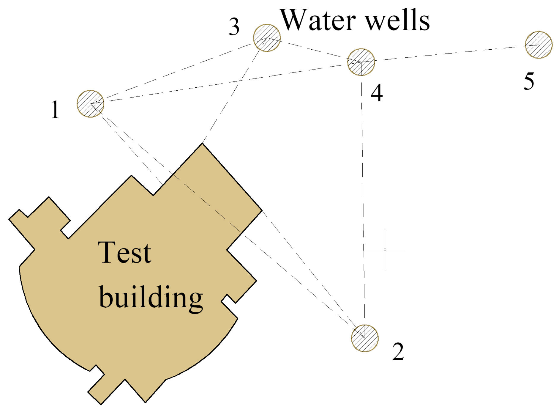
2.1. System Description and Data Monitoring
2.2. ANN Model
2.3. Detailed Model
- one-dimensional flow of refrigerant and secondary fluid;
- refrigerant pressure drop and viscous friction neglected in heat exchangers; and,
- only axial flows taken into account in heat exchanges.
2.4. DOE-2 Model
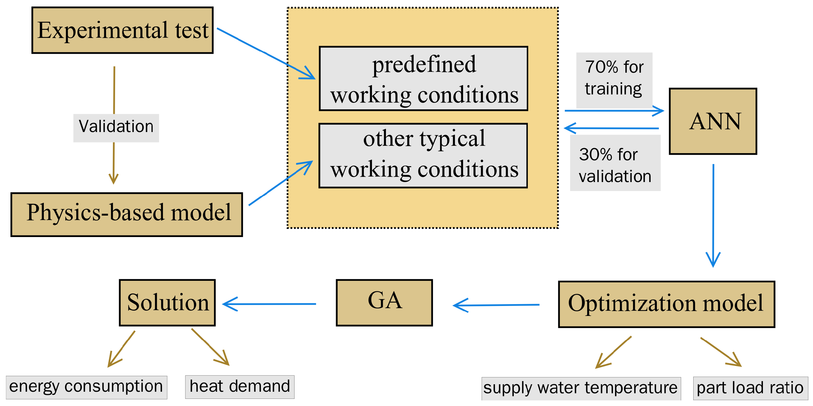
3. Optimization Model Formulation and Solving
3.1. Formulation
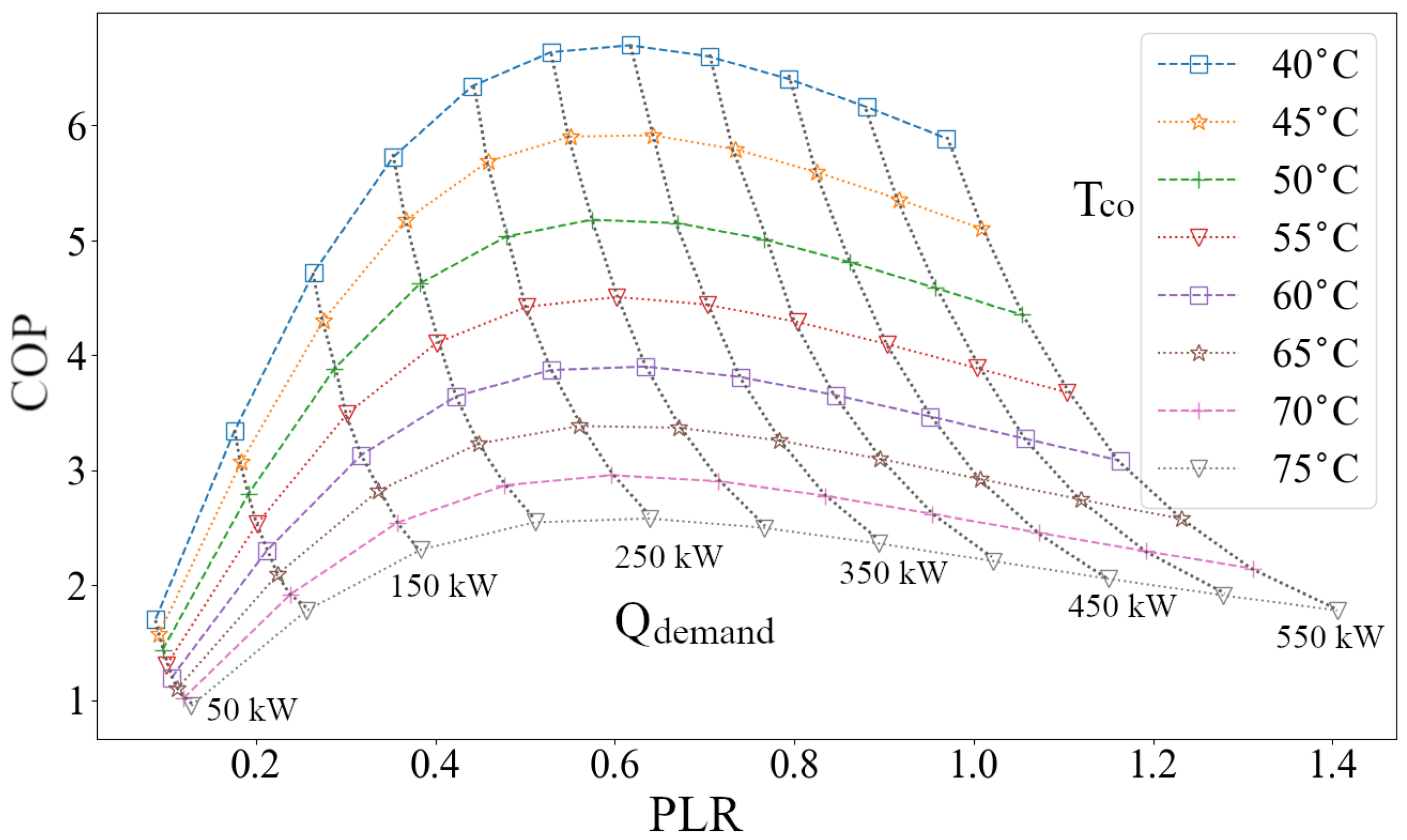
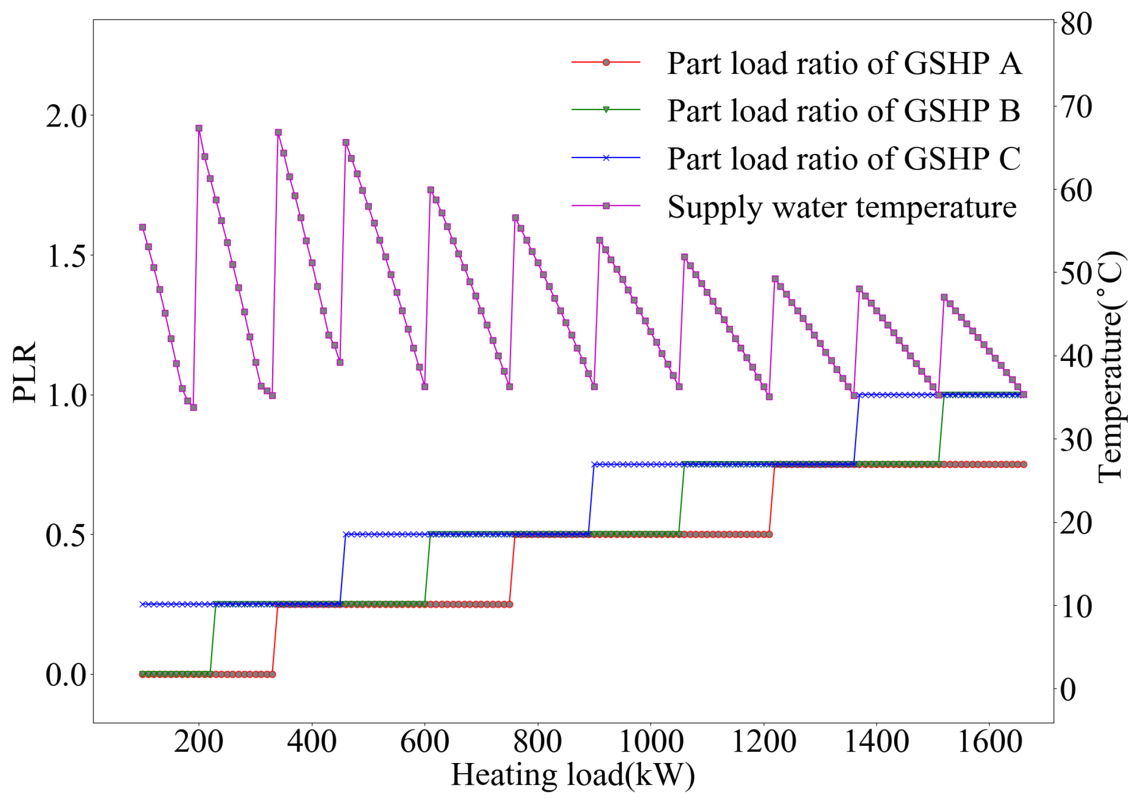
- Water supply temperatureFrom the performance analysis of the GSHP system, as shown in Figure 5, it could be concluded that a lower water supply temperature leads to higher COP of the system while providing the same amount of heating. However, the temperature range of supply water is restricted by the load capacity and operation mode of the indoor terminal units. The indoor terminal units operate automatically to satisfy the heating demand and maintain the temperature setpoint in each room. If the water supply temperature is too low, the output of the terminal units may be unable to meet the heating demand and desired indoor comfort even with full capacity. Thus, the optimization of water supply temperature depends not only on the system itself, but also on the external load conditions. An EnergyPlus model of the building, including the HVAC system, was setup to evaluate the supply water temperature range related to heating demand.
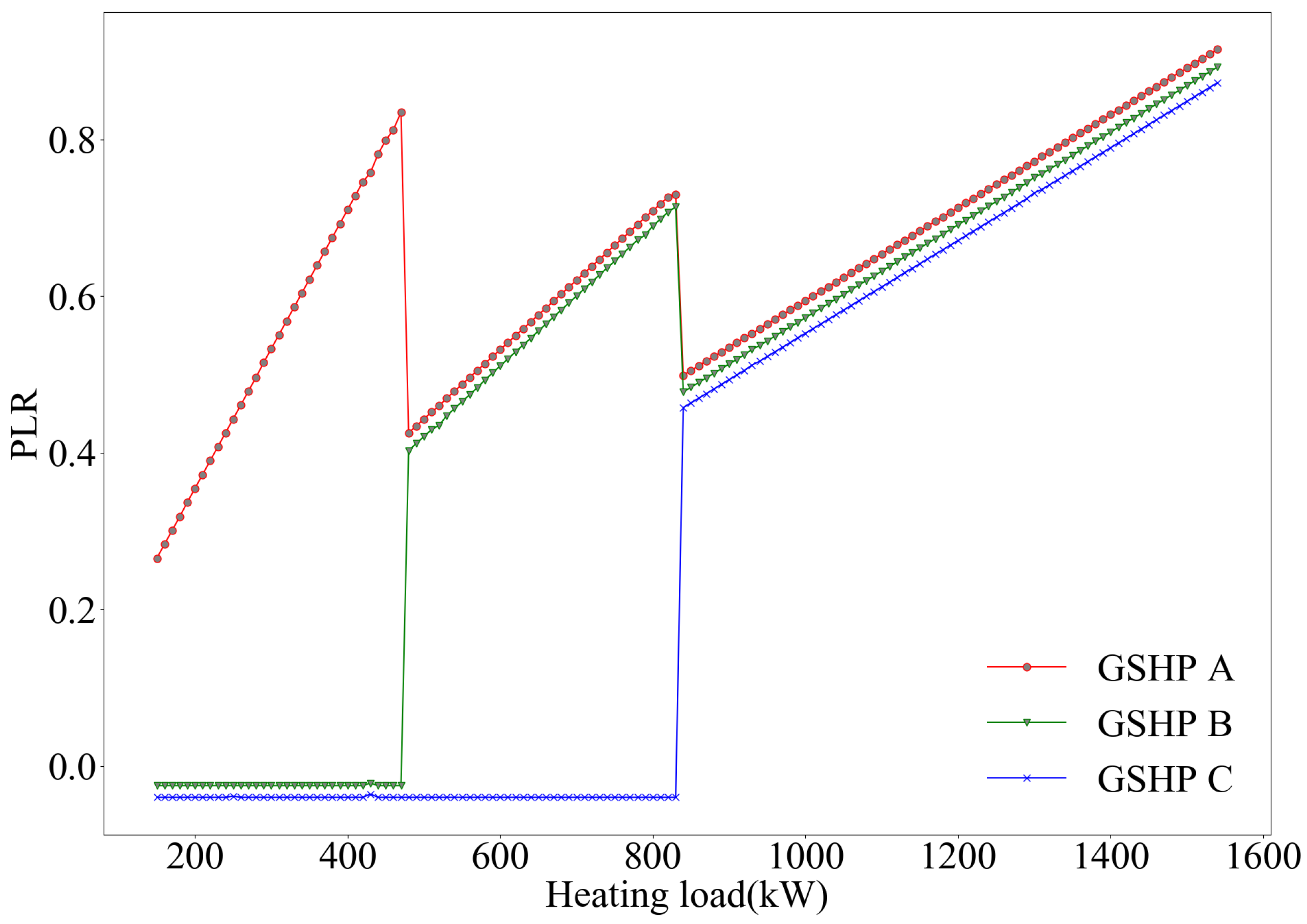
- GSHP stagingFor a fixed speed compressor, capacity control can be done by regulating slide valve position in the suction area to adjust the amount of refrigerant being compressed. On the basis of operation mode, the capacity control can be either continuous (from 10% to 100%) or staged with only several specific slide valve positions, like 25%, 50%, 75%, and 100%. Thus, the optimization of PLR depends on the part-load energy performance of GSHP.
3.2. Solving
4. Results and Discussion
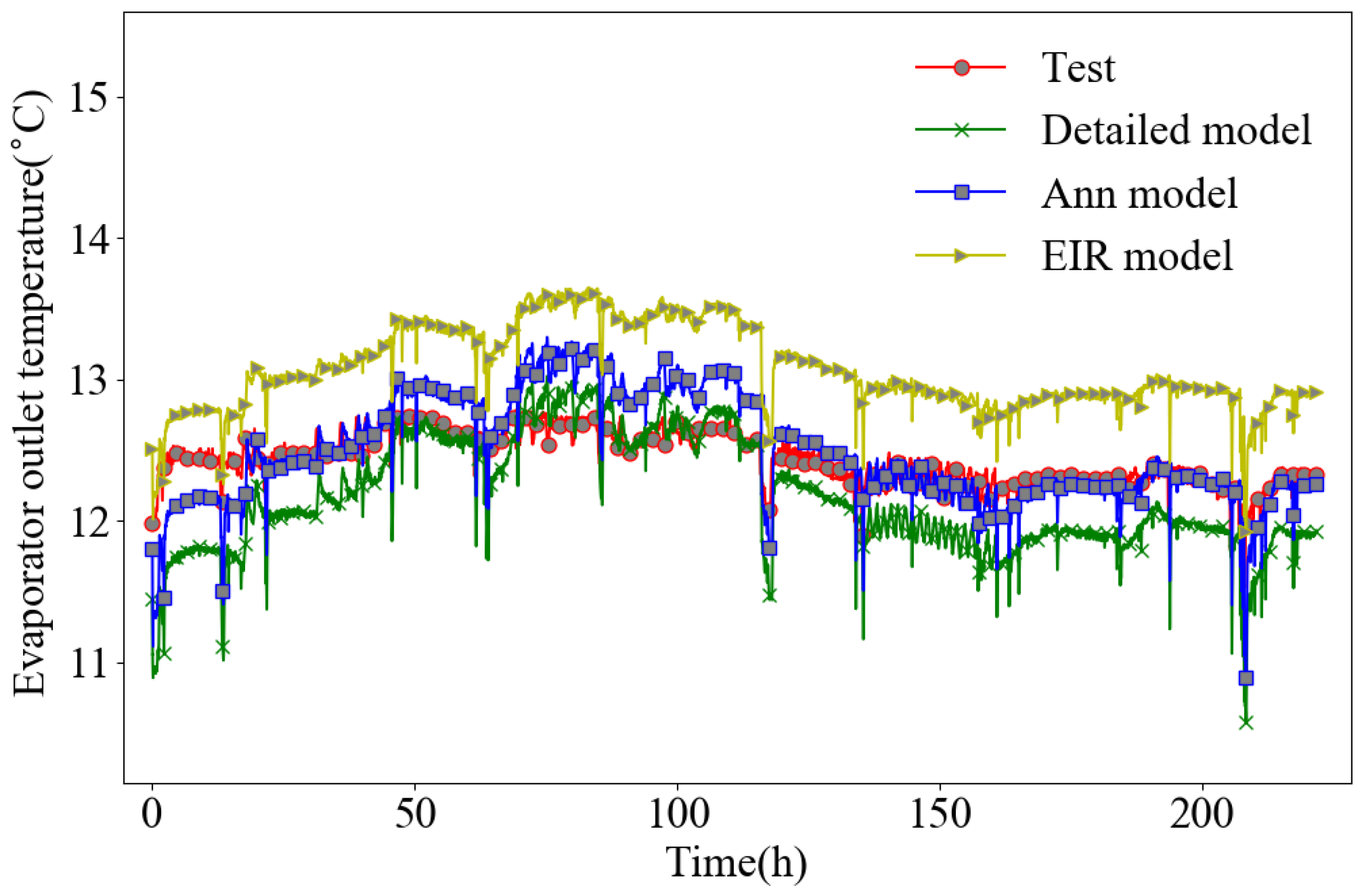
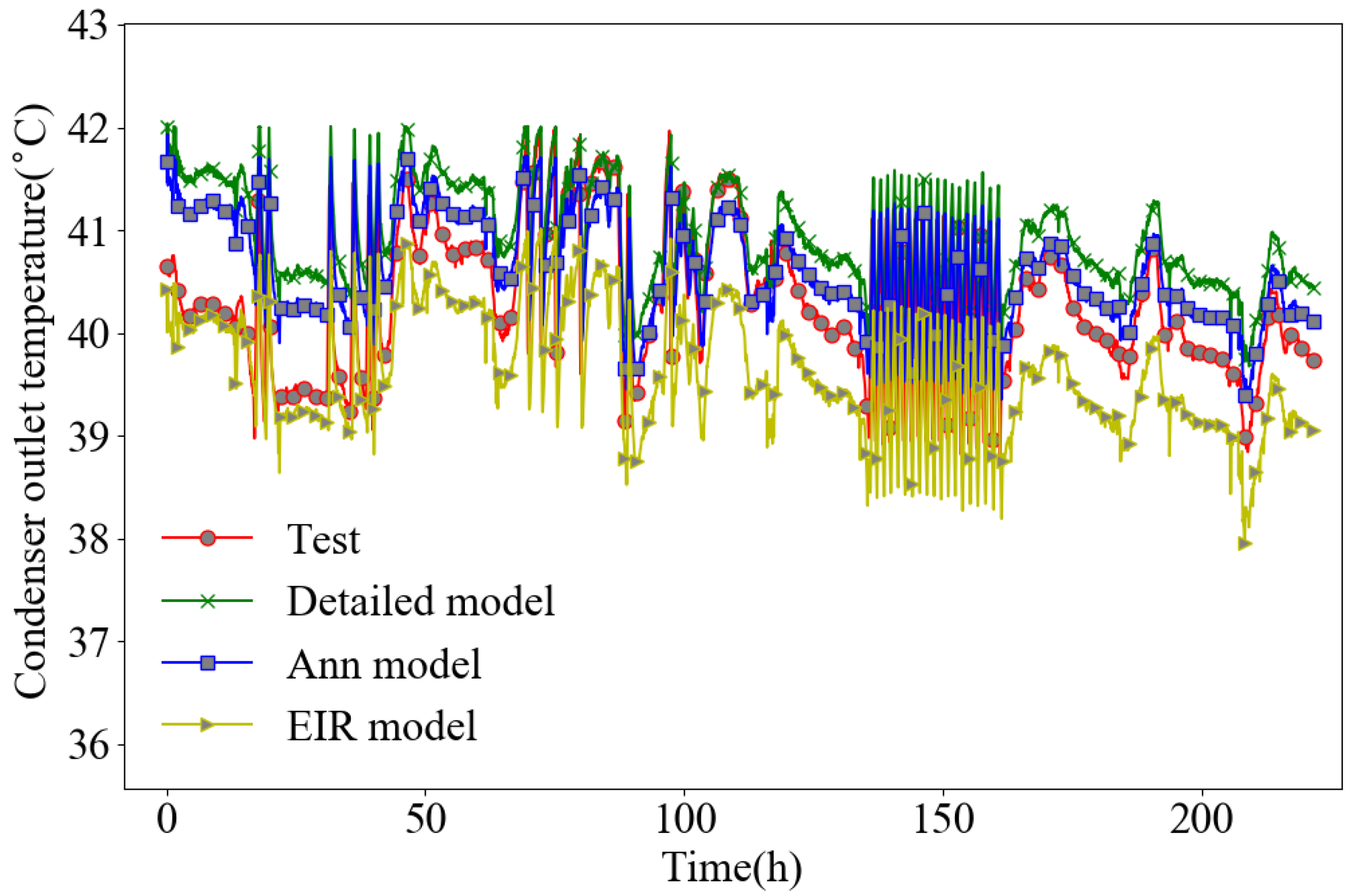
4.1. Experimental Analysis and Model Validation
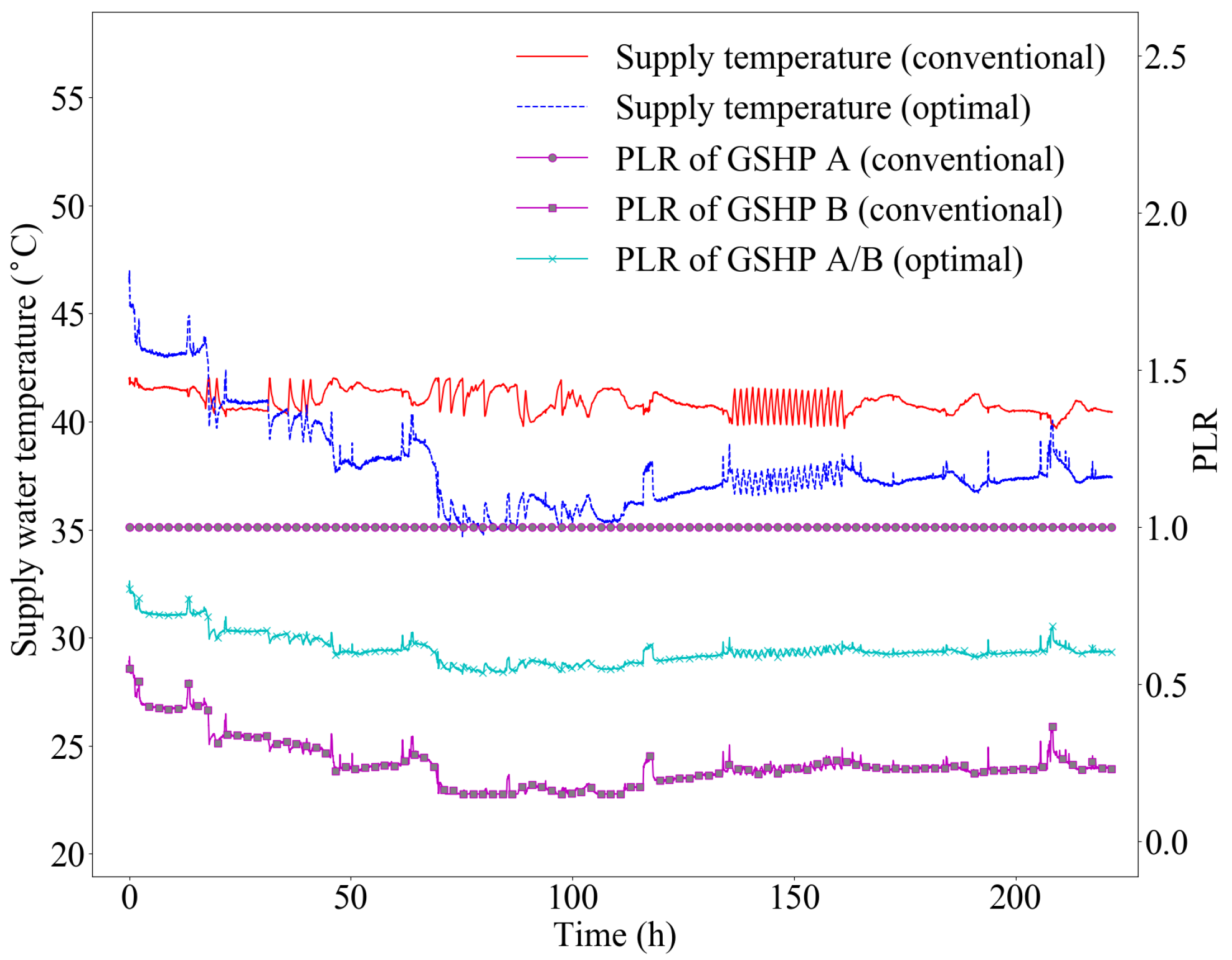
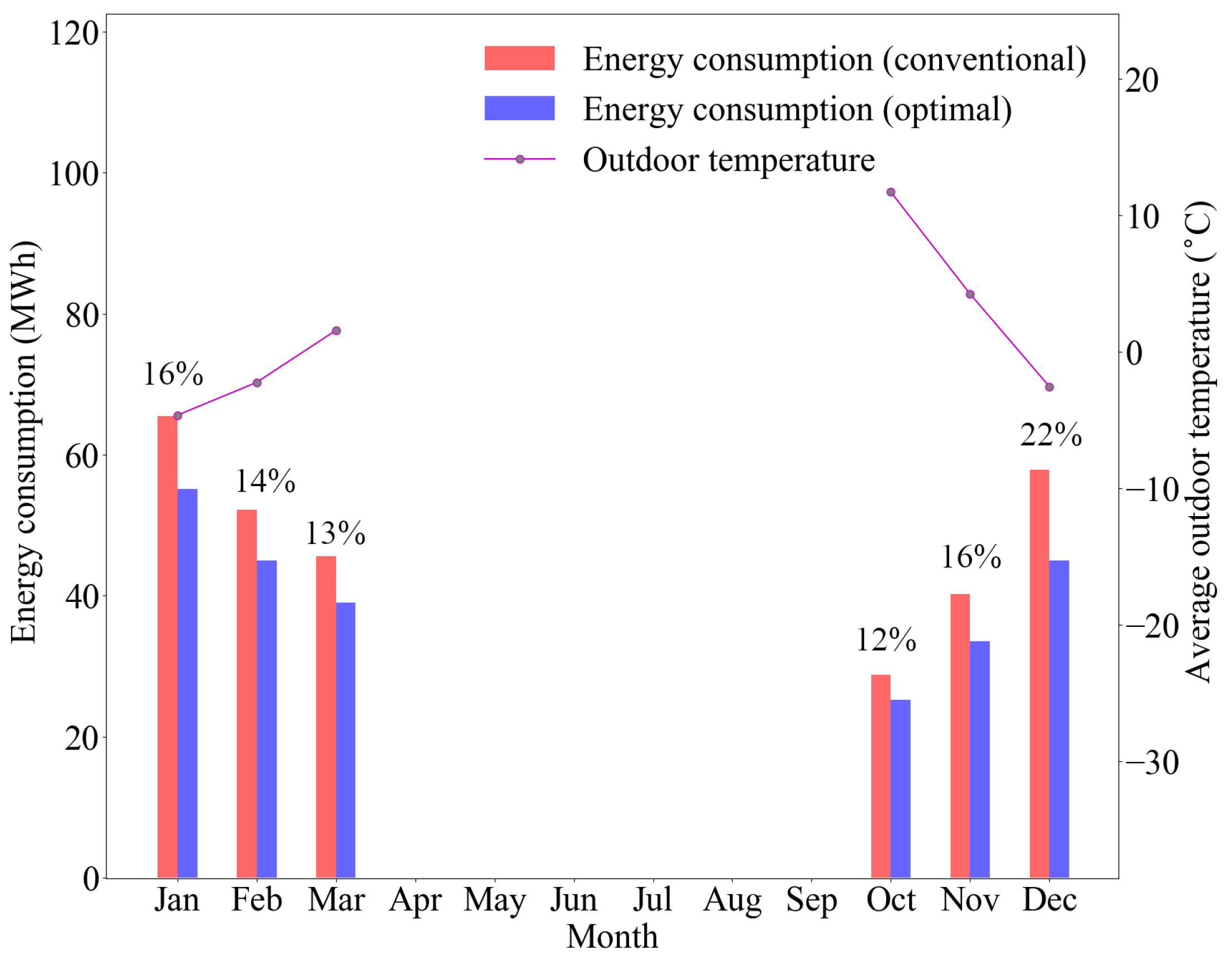
4.2. Optimized Operation Strategy
4.2.1. Water Supply Temperature
4.2.2. GSHP Staging
5. Conclusions
Author Contributions
Funding
Conflicts of Interest
List of Symbols
| Symbol | |
| density () | |
| u | velocity () |
| e | specific internal energy () |
| P | pressure () |
| Q | heat transfer rate () |
| T | temperature () |
| A | cross-sectional area () |
| D | tube diameter () |
| specific heat () | |
| m | flow rate () |
| time () | |
| z | length in the flow direction () |
| W | power consumption () |
| coefficients (-) | |
| objective function (-) | |
| Subscripts | |
| r | refrigerant |
| t | tube |
| w | water |
| i | inner |
| o | outer |
| evaporator outlet | |
| condenser outlet | |
| reference | |
| available | |
| heat pump | |
| c | evaporator |
| e | condenser |
| evaporator inlet | |
| condenser inlet | |
| Acronyms | |
| GSHP | ground source heat pump |
| ANN | artificial neural network |
| ANFIS | adaptive neuro-fuzzy inference system |
| HVAC | Heating, Ventilation and Air Conditioning |
| PLR | part load ratio (-) |
| COP | coefficient of performance (-) |
References
- Zeng, Y.; Zhang, Z.; Kusiak, A. Predictive Modeling and Optimization of a Multi-Zone HVAC System with Data Mining and Firefly Algorithms. Energy 2015, 86, 393–402. [Google Scholar] [CrossRef]
- Mossolly, M.; Ghali, K.; Ghaddar, N. Optimal Control Strategy for a Multi-Zone Air Conditioning System Using a Genetic Algorithm. Energy 2009, 34, 58–66. [Google Scholar] [CrossRef]
- Zhang, L.; Liu, X.; Jiang, Y. Application of Entransy in the Analysis of HVAC Systems in Buildings. Energy 2013, 53, 332–342. [Google Scholar] [CrossRef]
- Sakulpipatsin, P.; Itard, L.C.M.; van der Kooi, H.J.; Boelman, E.C.; Luscuere, P.G. An Exergy Application for Analysis of Buildings and HVAC Systems. Energy Build. 2010, 42, 90–99. [Google Scholar] [CrossRef]
- Vakiloroaya, V.; Ha, Q.P.; Samali, B. Energy-Efficient HVAC Systems: Simulation–Empirical Modelling and Gradient Optimization. Autom. Constr. 2013, 31, 176–185. [Google Scholar] [CrossRef] [Green Version]
- Sánta, R.; Garbai, L.; Fürstner, I. Optimization of Heat Pump System. Energy 2015, 89, 45–54. [Google Scholar] [CrossRef]
- Sun, W.; Hu, P.; Lei, F.; Zhu, N.; Jiang, Z. Case Study of Performance Evaluation of Ground Source Heat Pump System Based on ANN and ANFIS Models. Appl. Therm. Eng. 2015, 87, 586–594. [Google Scholar] [CrossRef]
- Esen, H.; Inalli, M. ANN and ANFIS Models for Performance Evaluation of a Vertical Ground Source Heat Pump System. Expert Syst. Appl. 2010, 37, 8134–8147. [Google Scholar] [CrossRef]
- Wang, J.; Li, G.; Chen, H.; Liu, J.; Guo, Y.; Sun, S.; Hu, Y. Energy Consumption Prediction for Water-Source Heat Pump System Using Pattern Recognition-Based Algorithms. Appl. Therm. Eng. 2018, 136, 755–766. [Google Scholar] [CrossRef]
- Gang, W.; Wang, J.; Wang, S. Performance Analysis of Hybrid Ground Source Heat Pump Systems Based on ANN Predictive Control. Appl. Energy 2014, 136, 1138–1144. [Google Scholar] [CrossRef]
- Kinab, E.; Marchio, D.; Rivière, P.; Zoughaib, A. Reversible Heat Pump Model for Seasonal Performance Optimization. Energy Build. 2010, 42, 2269–2280. [Google Scholar] [CrossRef]
- Alamin, Y.I.; Alvarez, J.D.; del Mar Castilla, M.; Ruano, A. An Artificial Neural Network (ANN) Model to Predict the Electric Load Profile for an HVAC System. IFAC Pap. 2018, 51, 26–31. [Google Scholar] [CrossRef]
- Guo, Y.; Wang, J.; Chen, H.; Li, G.; Liu, J.; Xu, C.; Huang, R.; Huang, Y. Machine Learning-Based Thermal Response Time Ahead Energy Demand Prediction for Building Heating Systems. Appl. Energy 2018, 221, 16–27. [Google Scholar] [CrossRef]
- Kusiak, A.; Xu, G.; Tang, F. Optimization of an HVAC System with a Strength Multi-Objective Particle-Swarm Algorithm. Energy 2011, 36, 5935–5943. [Google Scholar] [CrossRef]
- Kusiak, A.; Tang, F.; Xu, G. Multi-Objective Optimization of HVAC System with an Evolutionary Computation Algorithm. Energy 2011, 36, 2440–2449. [Google Scholar] [CrossRef]
- Kusiak, A.; Xu, G. Modeling and Optimization of HVAC Systems Using a Dynamic Neural Network. Energy 2012, 42, 241–250. [Google Scholar] [CrossRef]
- Kusiak, A.; Li, M.; Tang, F. Modeling and Optimization of HVAC Energy Consumption. Appl. Energy 2010, 87, 3092–3102. [Google Scholar] [CrossRef]
- He, X.; Zhang, Z.; Kusiak, A. Performance Optimization of HVAC Systems with Computational Intelligence Algorithms. Energy Build. 2014, 81, 371–380. [Google Scholar] [CrossRef]
- Wei, X.; Kusiak, A.; Li, M.; Tang, F.; Zeng, Y. Multi-Objective Optimization of the HVAC (Heating, Ventilation, and Air Conditioning) System Performance. Energy 2015, 83, 294–306. [Google Scholar] [CrossRef]
- Nassif, N. Modeling and Optimization of HVAC Systems Using Artificial Neural Network and Genetic Algorithm. Build. Simul. 2014, 7, 237–245. [Google Scholar] [CrossRef]
- Xia, L.; Ma, Z.; McLauchlan, C.; Wang, S. Experimental Investigation and Control Optimization of a Ground Source Heat Pump System. Appl. Therm. Eng. 2017, 127, 70–80. [Google Scholar] [CrossRef]
- Sivasakthivel, T.; Murugesan, K.; Thomas, H.R. Optimization of Operating Parameters of Ground Source Heat Pump System for Space Heating and Cooling by Taguchi Method and Utility Concept. Appl. Energy 2014, 116, 76–85. [Google Scholar] [CrossRef]
- Gao, J.; Huang, G.; Xu, X. An Optimization Strategy for the Control of Small Capacity Heat Pump Integrated Air-Conditioning System. Energy Convers. Manag. 2016, 119, 1–13. [Google Scholar] [CrossRef] [Green Version]
- Cervera-Vazquez, J.; Montagud, C.; Corberan, J.M. In Situ Optimization Methodology for Ground Source Heat Pump Systems: Upgrade to Ensure User Comfort. Energy Build. 2015, 109, 195–208. [Google Scholar] [CrossRef]
- Hussain, S.; Gabbar, H.A.; Bondarenko, D.; Musharavati, F.; Pokharel, S. Comfort-Based Fuzzy Control Optimization for Energy Conservation in HVAC Systems. Control Eng. Pract. 2014, 32, 172–182. [Google Scholar] [CrossRef]
- Esen, H.; Turgut, E. Optimization of Operating Parameters of a Ground Coupled Heat Pump System by Taguchi Method. Energy Build. 2015, 107, 329–334. [Google Scholar] [CrossRef]
- Bendapudi, S. Development and Evaluation of Modeling Approaches for Transients in Centrifugal Chillers. Ph.D. Thesis, University of Wisconsin, Madison, WI, USA, 2004. [Google Scholar]
- Bendapudi, S.; Braun, J.E.; Groll, E.A. A Comparison of Moving-Boundary and Finite-Volume Formulations for Transients in Centrifugal Chillers. Int. J. Refrig. 2008, 31, 1437–1452. [Google Scholar] [CrossRef]
- Hydeman, M.; Gillespie, K.L., Jr.; Dexter, A. Tools and Techniques to Calibrate Electric Chiller Component Models. ASHRAE Trans. 2002, 108, 733–741. [Google Scholar]
- Yuan, S.; Grabon, M. Optimizing Energy Consumption of a Water-Loop Variable-Speed Heat Pump System. Appl. Therm. Eng. 2011, 31, 894–901. [Google Scholar] [CrossRef]
- Jeon, J.; Lee, S.; Hong, D.; Kim, Y. Performance Evaluation and Modeling of a Hybrid Cooling System Combining a Screw Water Chiller with a Ground Source Heat Pump in a Building. Energy 2010, 35, 2006–2012. [Google Scholar] [CrossRef]


| Components | Parameters | Values |
|---|---|---|
| ground source heat pumps | Nominal heating capacity | 545.3 kW |
| Nominal cooling capacity | 401.4 kW | |
| Nominal power consumption for heating | 107.3 kW | |
| Nominal power consumption for cooling | 82.7 kW | |
| underground water pumps | 65 | |
| circulating pumps | 80 | |
| Refrigerant | R22 |
| Models | RMS | Computational Time | |
|---|---|---|---|
| Detailed | 0.7729 | 0.9408 | 3~5 s for each timestep |
| ANN | 0.7903 | 0.9378 | 171 ms for whole simulation |
| DOE-2 | 1.2032 | 0.9102 | 2.2 ms for whole simulation |
© 2020 by the authors. Licensee MDPI, Basel, Switzerland. This article is an open access article distributed under the terms and conditions of the Creative Commons Attribution (CC BY) license (http://creativecommons.org/licenses/by/4.0/).
Share and Cite
Wang, G.; Wang, H.; Kang, Z.; Feng, G. Data-Driven Optimization for Capacity Control of Multiple Ground Source Heat Pump System in Heating Mode. Energies 2020, 13, 3595. https://doi.org/10.3390/en13143595
Wang G, Wang H, Kang Z, Feng G. Data-Driven Optimization for Capacity Control of Multiple Ground Source Heat Pump System in Heating Mode. Energies. 2020; 13(14):3595. https://doi.org/10.3390/en13143595
Chicago/Turabian StyleWang, Guiqiang, Haiman Wang, Zhiqiang Kang, and Guohui Feng. 2020. "Data-Driven Optimization for Capacity Control of Multiple Ground Source Heat Pump System in Heating Mode" Energies 13, no. 14: 3595. https://doi.org/10.3390/en13143595
APA StyleWang, G., Wang, H., Kang, Z., & Feng, G. (2020). Data-Driven Optimization for Capacity Control of Multiple Ground Source Heat Pump System in Heating Mode. Energies, 13(14), 3595. https://doi.org/10.3390/en13143595