Abstract
Electro-hydraulic excitation systems are key equipment in various industries. Electric motor driving rotary valves are mostly used in existing systems. However, due to the separate design of the driving and hydraulic parts, highly compact integration cannot be achieved by these type of systems. Moreover, investigation on the influence of relevant parameters on the system has been insufficient in previous studies. To overcome these problems, a novel full electro-hydraulic excitation system scheme as well as a parameters analysis are presented in this paper. Theoretical models of the flow areas for valve orifices of different geometric shapes are obtained, based on which an AMESim® simulation model of the system is established. The effects of the main parameters are analyzed using numerical simulations, and the coupling relationship of the parameters is revealed. The results demonstrate the feasibility and effectiveness of the proposed method. Experimental studies were conducted to verify the effectiveness of the proposed system scheme and the analysis results. We found that a highly compact integration can be obtained while maintaining a high reversing frequency. We also found that the proposed system has a certain level of load adaptability, which is superior to the existing methods.
1. Introduction
Electro-hydraulic vibration technology is an indispensable basic technology widely used in the automation, aerospace, construction machinery, and military fields [1,2,3,4]. The working process of the electro-hydraulic vibration exciter (EHVE) is as follows. Drive signals are input to the electromagnetic directional valve to achieve high-speed reversing, whereas the hydraulic cylinder is controlled to reciprocate with high speeds to realize vibration. According to the working principle of the EHVE, the control valve is the key component, whose performance directly determines the operational quality of the EHVE.
Servo valves have been widely used in most EHVEs before 2006 [5,6,7]. However, there are several limitations on the servo valve in the context of EHVE, such as serious waveform distortion and limited vibration frequency (less than 50 Hz). Electric motor driving rotary valve based solutions are widely considered by researchers in the literature as the most important approach to overcome these problems [8,9,10,11,12,13,14,15,16,17,18]. Sallas [8] developed a low inertia servo valve that set the reversing frequency to 160 HZ. However, the structure of the valve core was complex for processing and the rotational inertia was large when the valve’s cavity was filled with hydraulic oil. Leonard et al. [9] proposed a rotary shaft type hydraulic valve, which reduced the spool’s driving torque and pre electromechanical converter power. However, this structure also reduced the vibration frequency’s efficiency and controllability. Griffin et al. [10] designed a rotary plate type valve that achieved a high reversing frequency, but the valve was only suitable for cases where pressures were not very high. Lu [11] contributed a limited-angle rotating of an electro-hydraulic servo-valve, which had a simple structure and set the reversing frequency at up to 120 HZ. Zhang et al. [12] developed a balanced stepped hydraulic rotary valve that obtained a higher reversing frequency and reduced the hydraulic oil leakage, but it is mainly applied to situations with high pressures and large flows. Ruan et al. [13,14,15] proposed an electro-hydraulic exciter controlled by a two dimensional valve that greatly improved the excitation frequency up to 200 HZ. However, the exciter had to design a special drive motor controller, which made the motor control circuits and the control algorithms more complex and only analyzed the influence of parameters including supply pressures and spool structures on the vibration waveform. Haidegger et al. [16] proposed a proportional-integral-derivative fuzzy controller’s application solution and Precup et al. [17] developed a stable fuzzy logic controller’s concept, which are useful for the controller’s design of the electric motor. Han et al. [18] developed a new electro-hydraulic exciter with different spools, showing advantages including a simple structure, a design free of a motor controller, and a high frequency up to 300 Hz.
In the existing systems, most of the high speed rotary directional control valves are driven by the electric motor to rotate the spool to achieve a high frequency switching of the flow port. These electro-hydraulic excitation systems overcome the limitation of the spool reciprocating structure on the bandwidth, based on previous study [19]. However, practical engineering applications require more simplified and integrated drive and control system structures, and the separate design of the driving and hydraulic parts cannot achieve a highly compact integration with this type of systems. Moreover, the importance of parameters analysis to the vibration waveform control is far beyond the scope of system development, and the investigation regarding the effects of relevant parameters on the system has been insufficient in previous studies, which mainly focused on structural parameters’ effects. Additionally, parameters’ relationships are not motivated by the above observations. This paper aims to propose a novel full electro-hydraulic excitation system scheme. Many parameters affect the system’s output vibration waveform, such as the valve spool rotation speed, orifice number, supply pressure, orifice shape, orifice axial length, transient flow torque, and load, to mention but a few. To achieve accurate waveforms, the effects of the main parameters are analyzed, and the coupling relationship of the parameters is revealed.
2. System Design Overview
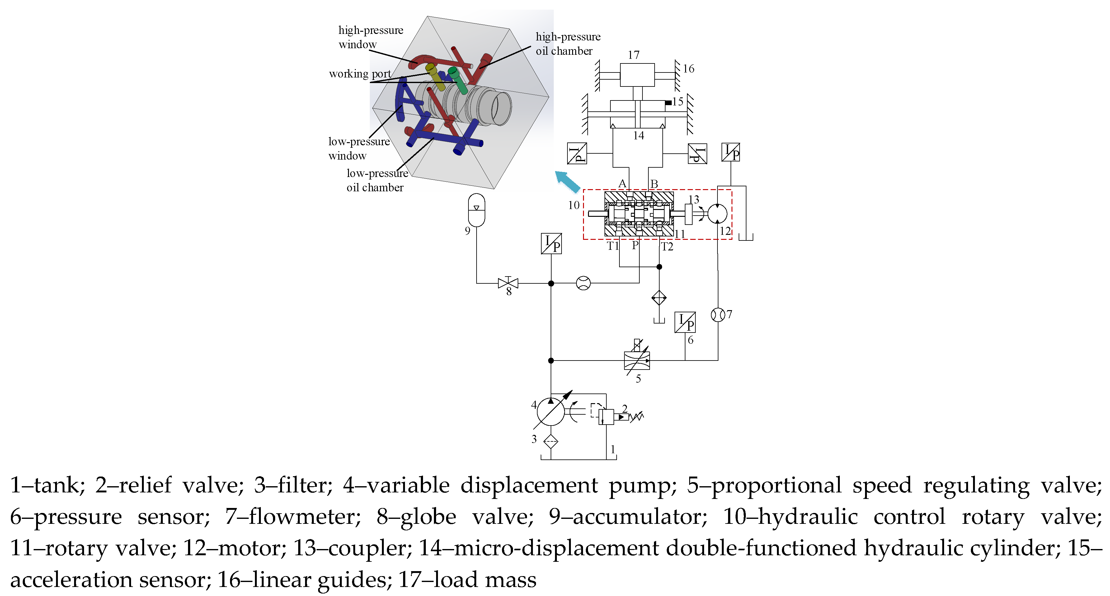
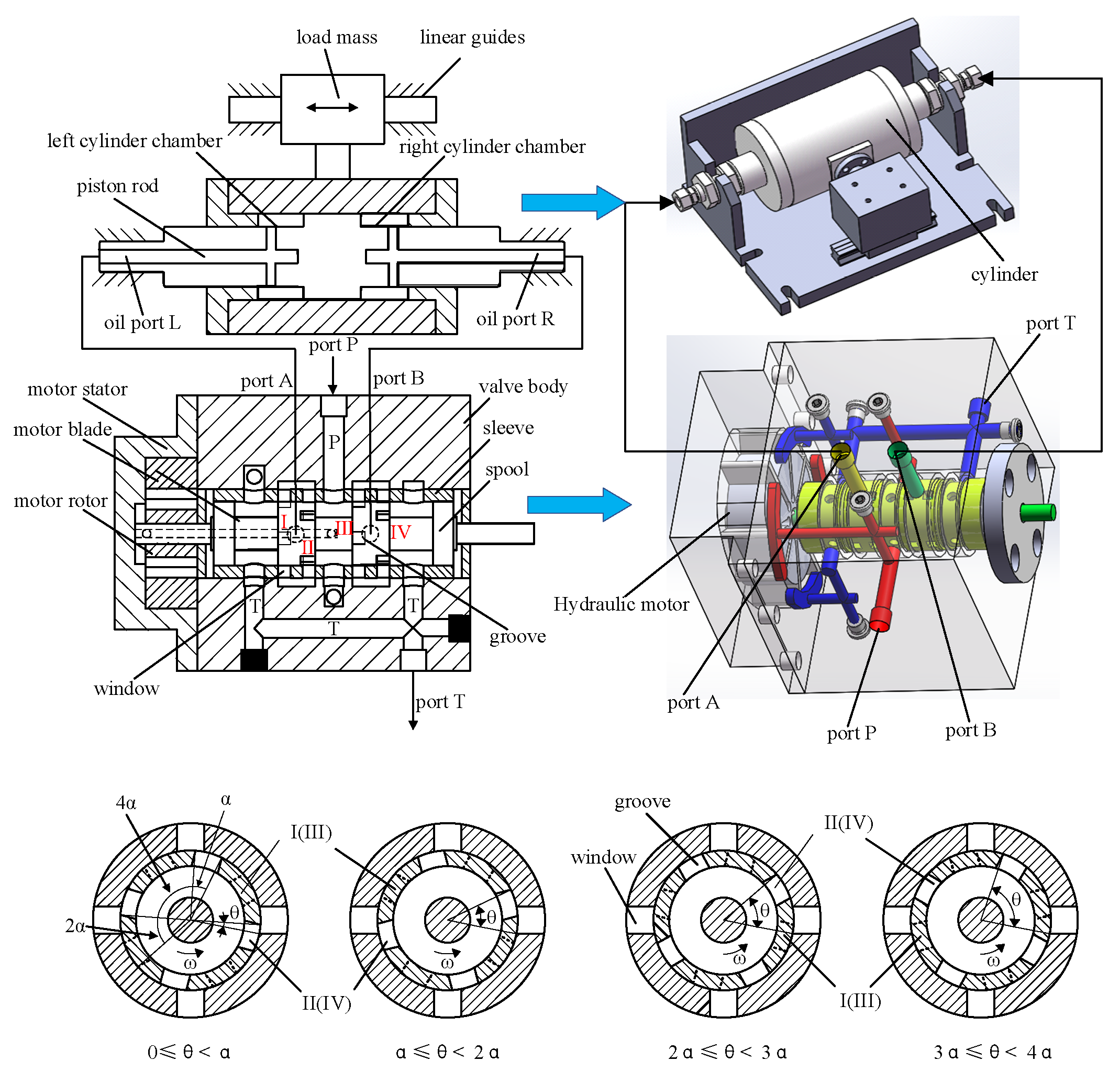
A prototype model of the hydraulic controlled rotary valve (HCRV) excitation system is shown in Figure 1. Component 10 represents the HCRV prototype model, which consists of elements 11, 12, and 13. The 3D diagram indicated by the blue arrow shows the designed HCRV [20]: the hydraulic oil enters the high pressure oil chamber and a portion of the oil enters the drive end of the HCRV to actuate the rotary valve spool to rotate (the drive end equals to a motor), while the other enters the rotary valve part of the HCRV and then enters the micro-displacement double-functioned hydraulic cylinder to realize excitation. The HCRV prototype model consists of a hydraulic motor and a rotary valve, which are connected through a coupler.
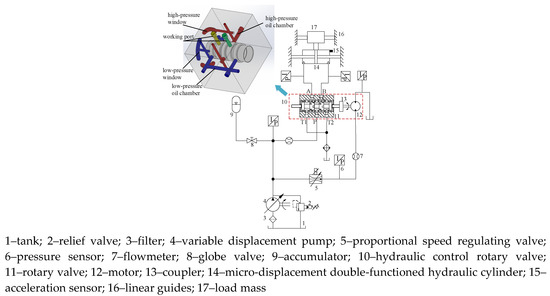
Figure 1.
Hydraulic controlled rotary valve excitation system.
The working process of the HCRV exciter is shown in Figure 2. The exciter controlled by the HCRV is composed of a HCRV and a micro-displacement double-functioned hydraulic cylinder. Taking the rotary valve with rectangular orifice as an example: there are two identical spool lands on the rotary spool. Each land has four identical rectangular grooves evenly distributed along the circumference direction. The valve sleeve is fitted with a rectangular window corresponding to the spool groove, and the valve ports are formed by the overlapping part between the valve sleeve windows and spool grooves, which are labeled as ports I, II, III, and IV. Valve ports I and IV are meter-in ports while ports II and III are meter-out oil ports. The variation of the flow area of valve ports I and III is the same as that of ports II and IV. Defining α as the central angle of one groove, 4α could be considered as the central angle between two adjacent grooves in geometry. On one spool land, the central angle between adjoining grooves belonging to different groups is 2α. The cylinder is controlled by the HCRV. When the hydraulic system starts to work, the hydraulic oil enters the high pressure oil chamber, a portion of the oil enters the HCRV drive end to actuate the rotary valve spool to rotate (the drive end is similar to a hydraulic motor), while the other enters the rotary valve part of the HCRV; the cylinder barrel is then driven to perform a reciprocating motion. The oil ports are set in the piston rod of the cylinder. The waveform of the HCRV excitation system is formed by the displacement change of the cylinder barrel.
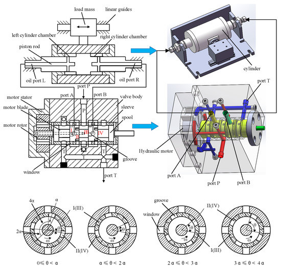
Figure 2.
Working process of the hydraulic controlled rotary valve exciter.
The specific working process of the HCRV exciter is as follows. The valves port flow area changes periodically in the process of spool rotation. When the angular displacement θ increases from 0 to α, valve ports II and IV remain open and their flow areas increase from zero to the maximum, while valve ports I and III remain closed. When the angular displacement increases from α to 2α, the flow area of valve ports II and IV decreases from the maximum to zero, while ports I and III remain closed. In this process, supply port P is connected to port A, whereas port B is connected to meter-out port T. The hydraulic oil enters the high pressure oil chamber (port P), and a portion of the oil enters the drive end of the HCRV to rotate the rotary valve spool (the drive end is similar to a hydraulic motor); the remaining oil enters the rotary valve through port P, valve port II, port A, and oil port L, and then enters the left cylinder chamber successively. The load mass driven by the cylinder barrel moves to the left side along the linear guides, and the oil in the right cylinder chamber flows back into the fuel tank through oil port R, port B, port IV of the value, and port T, successively.
Similarly, when the angular displacement θ changes from 2α to 3α, valve ports I and III remain open and their flow areas increase from zero to the maximum, while valve ports II and IV remain closed. When the angular displacement increases from 3α to 4α, the flow areas of valve ports I and III decrease from the maximum to zero, while ports II and IV remain closed. In this process, port P is connected to port B, whereas port A is connected to meter-out port T. One part of the hydraulic oil still enters the motor and drives the rotary valve spool to rotate, and the remaining oil enters the rotary valve successively through port P, valve port III, port B, and oil port R, and then enters the right cylinder chamber. The load mass driven by the cylinder barrel moves to the right along the linear guides and the oil in the left cylinder chamber flows back to the fuel tank through oil port L, port A, valve port I, and port T, successively.
The structures and working principles of the triangular and semicircular valves are the same as that of the rectangular valve.
3. Modeling of the System
To determine the rotation direction conveniently, the displacement of the cylinder is defined as positive when moving to the left and negative when moving to the right; thus, the range of the rotation angle displacement is changed from to .
Therefore, when , the theoretical model of flow areas for the rectangular orifice is shown in Equation (1) [21]; when , Equation (1) is rewritten as Equation (2):
where is the axial width of the rectangular orifice, N is the number of the groove, r is the valve spool radius, and α is the central angle of one groove, according to the rotary valve’s geometric structure, .
Rewriting the equation of flow areas change for triangular orifice as (4), corresponding to (3):
where is the axial width of the triangular orifice.
Reformulating the equation of flow areas for the semicircular orifice from (5) into (6):
where is the axial width of the semicircular orifice, and .
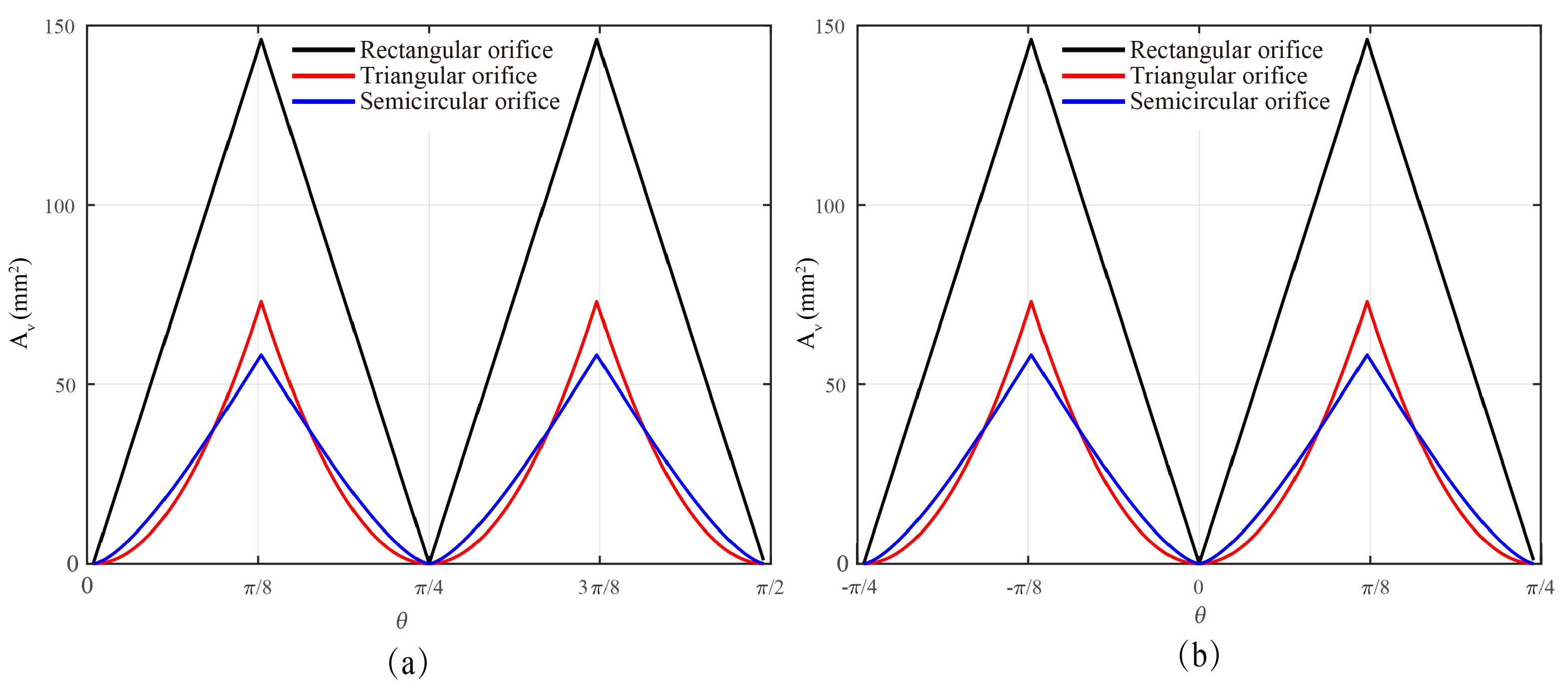
In the case of , the rectangular, triangular, and semicircular orifice flow areas as Equations (1), (3), and (5) are shown in Figure 3a. After reformulating , these flow areas under different orifices described through Equations (2), (4), and (6) are shown in Figure 3b. It can be seen that the flow areas of the rotary valve with different orifices remain unchanged, which reflects the correctness of Equations (2), (4), and (6).
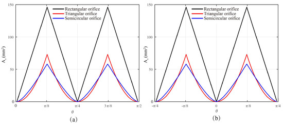
Figure 3.
Orifice flow areas: (a) in , (b) in .
Based on the Equations (2), (4), and (6), an AMESim® model of the HCRV excitation system was established. By referring to relevant literature [22,23], a slide valve model was selected to replace the rotary valve, and it was necessary to ensure that the change rule of the slide valve port flow areas is consistent with that of the rotary valve. The relevant parameters related to the valve port flow area in AMESim® are the diameter and the axial displacement of the spool, which can be described by the following equation:
Assuming that the diameter of the slide valve is the same as that of the rotary valve, , the maximum displacement can be obtained by Equation (8).
The reversing period of the slide valve spool model should be the same as that of the rotary valve, so the relationship between the axial displacement x and the rotation speed n of the rotary valve spool can be calculated easily.
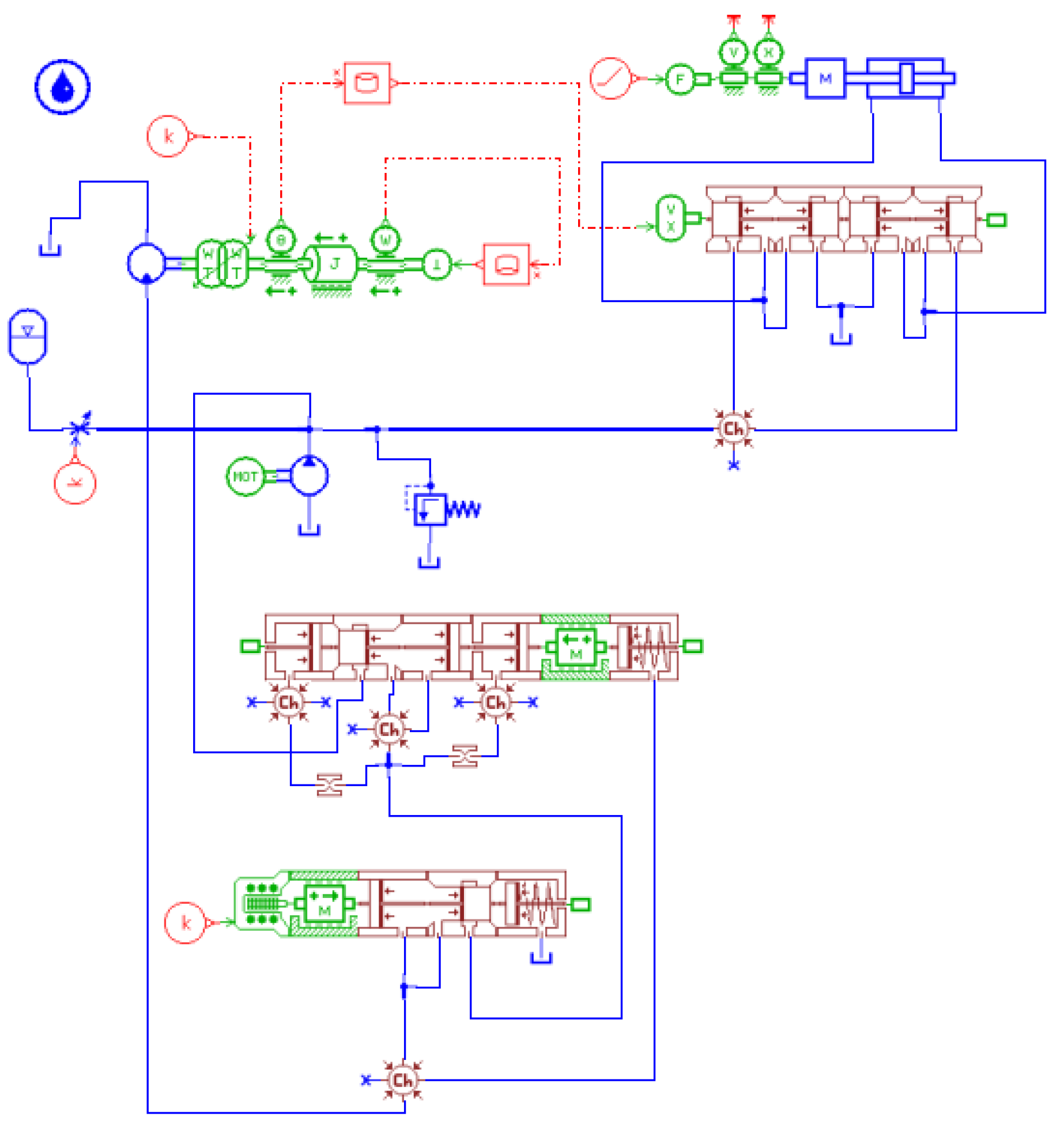
The simulation model of the HCRV excitation system constructed in the simulation platform AMESim® is shown in Figure 4 and the corresponding main parameters are given in Table 1.
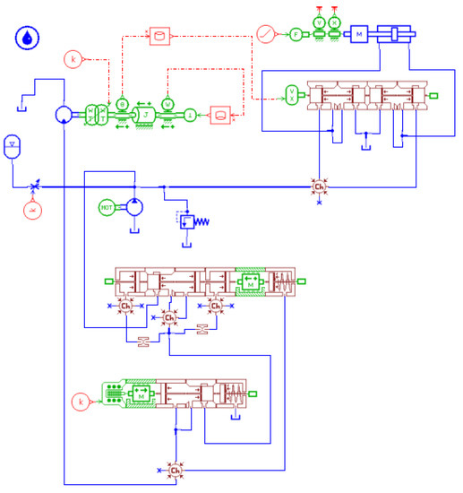
Figure 4.
Simulation model of the hydraulic controlled rotary valve excitation system.

Table 1.
Main parameters of the simulation model.
4. Simulation Results and Parameters Analysis
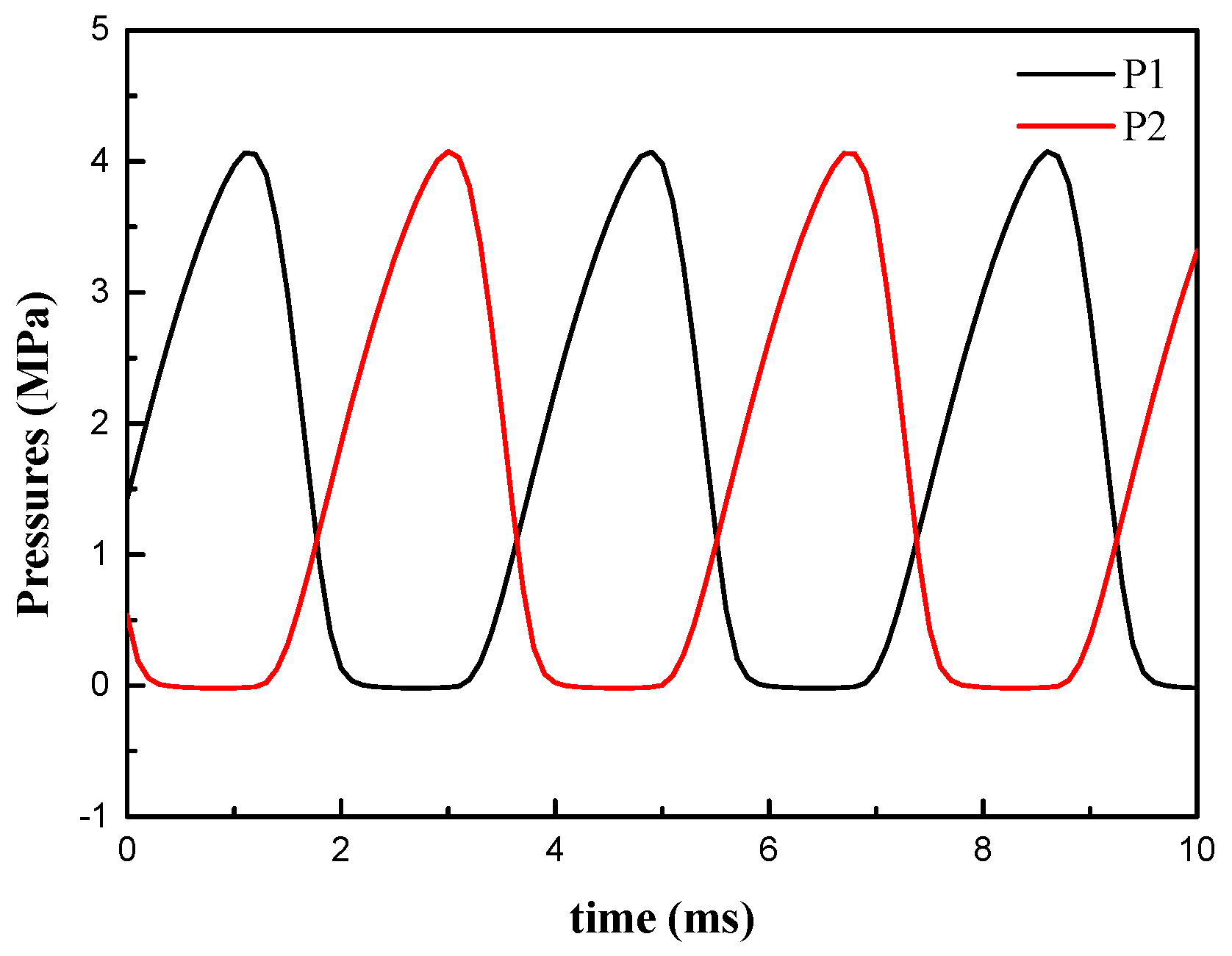
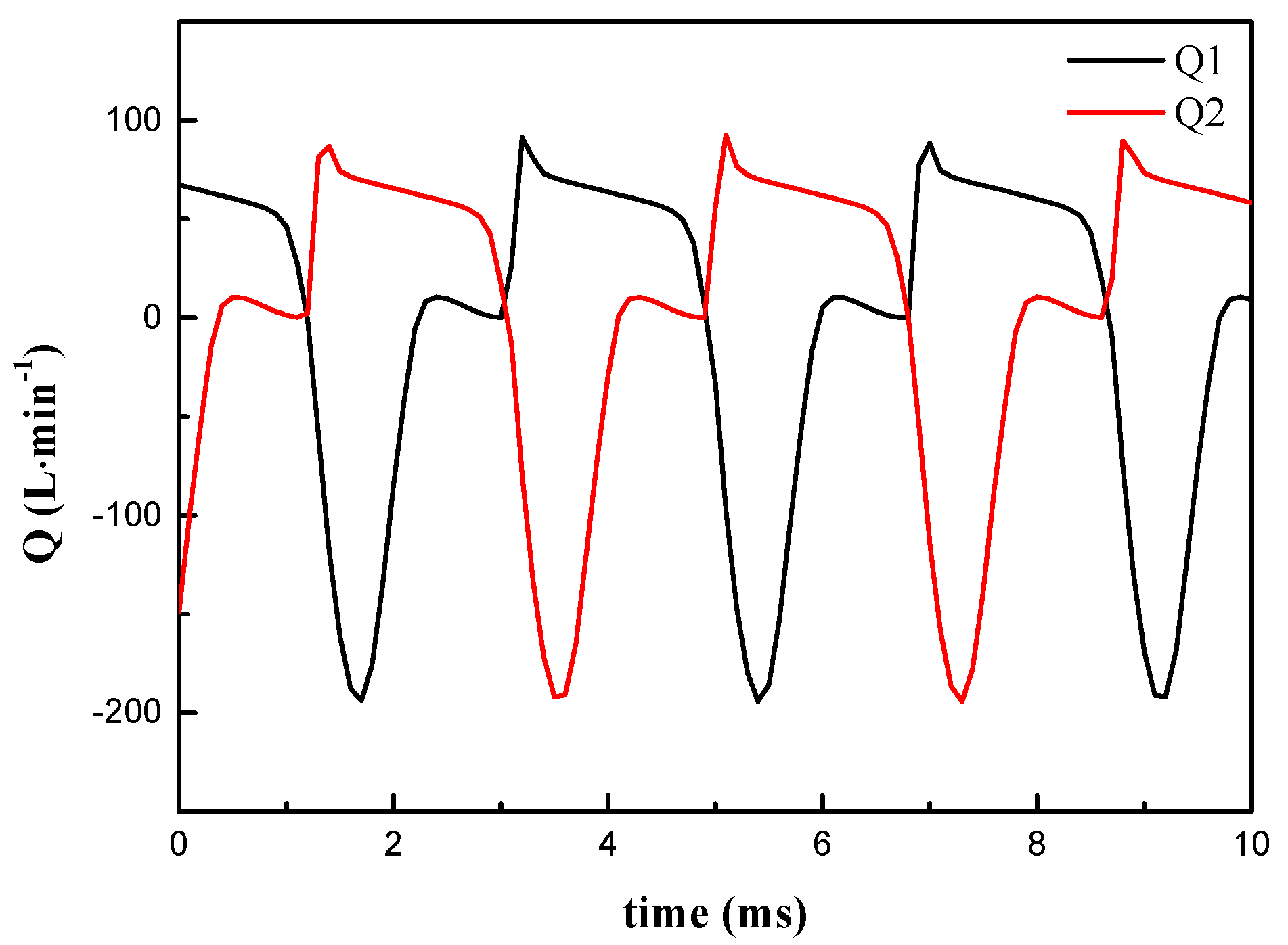
Figure 5 and Figure 6 show pressures and flows of the hydraulic cylinder’s two chambers. In a steady state, the pressure and flow waveforms of the cylinder’s two chambers are symmetrical to each other and the phase difference is 0.002 s. However, as soon as the rotary valve reverses, the valve port flow will increase significantly, and such instantaneous flow will exceed the system oil supply flow even after several times, which can momentarily lead to a strong hydraulic impact. Therefore, a proportional flow control valve is introduced into the HCRV excitation system to damp the hydraulic impact.

Figure 5.
Pressures of hydraulic cylinder’s two chambers.
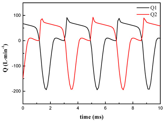
Figure 6.
Flows of hydraulic cylinder’s two chambers.
The main parameters that influence the waveform of the HCRV excitation system include the spool rotation speed, oil supply pressure, orifice number, orifice shape, orifice axial length, transient flow torque, and load mass.
4.1. The Influence of Different Spool Rotation Speeds on the Excitation Waveform
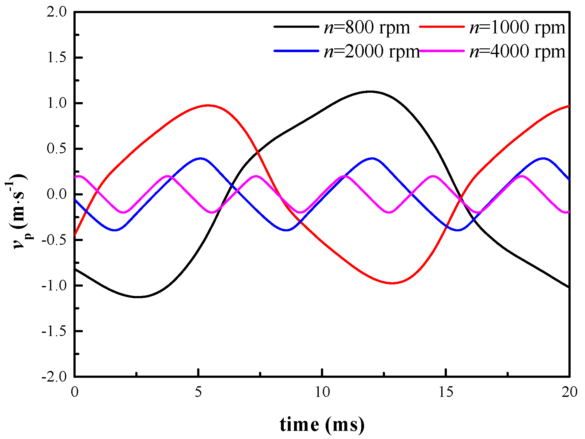
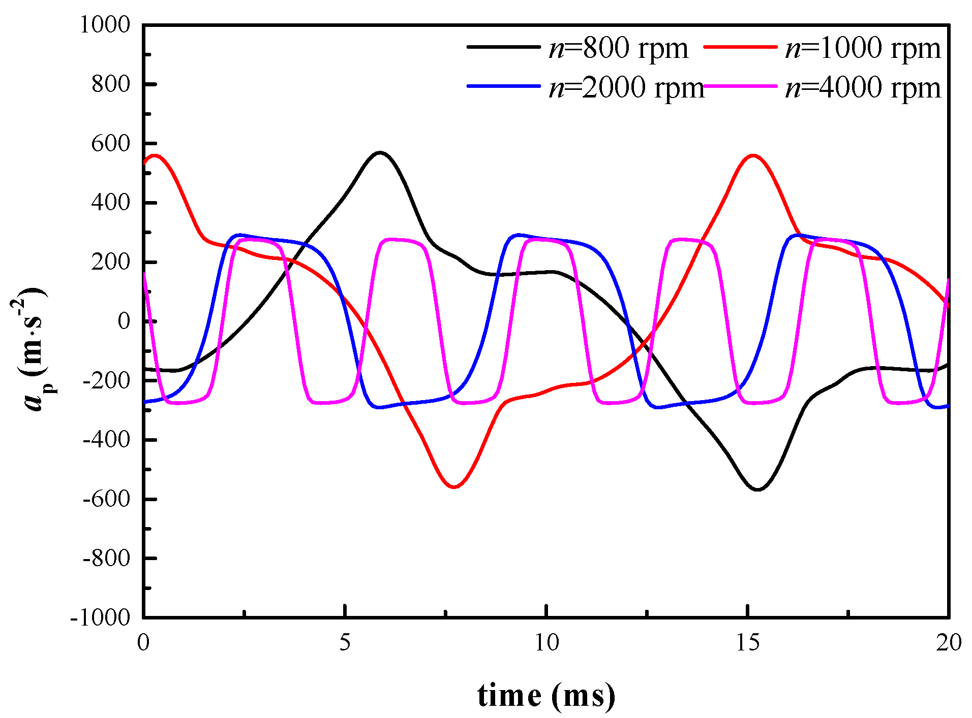
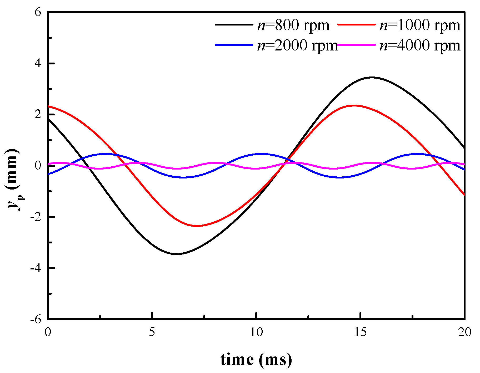
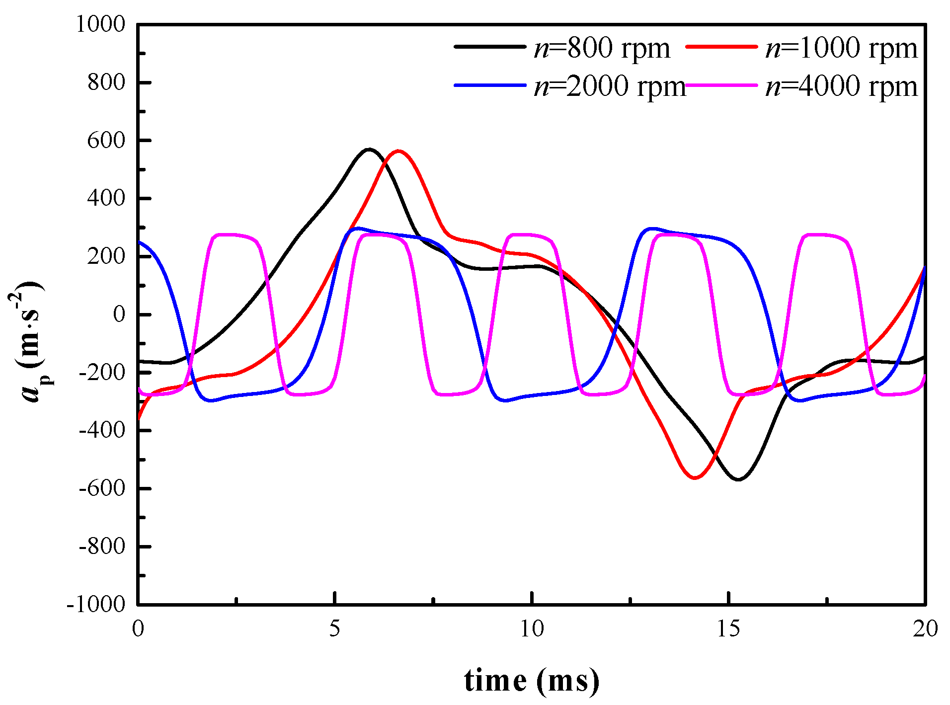
From the formula [21], when the orifice number is constant, the reversing frequency of the HCRV exciter is proportional to the spool rotation speed, that is, as the spool rotation speed increases, the reversing frequency of the HCRV exciter increases, and vice versa. It can be seen from Figure 1 that the spool rotation speed is positive in relation to the proportional flow control valve opening and the oil supply pressure; this is because the change in the valve opening or the supply pressure changes the flow rate, which in turn changes the hydraulic motor speed; thus the simulation analysis is carried out in two cases separately. When the proportional flow control valve port is fully open, the relationships of the rotation speed with the displacement , velocity , and acceleration of the HCRV excitation system are shown in Figure 7, Figure 8 and Figure 9. When the supply pressure is 4 MPa, the relationships of the rotation speed to the displacement , velocity , and acceleration of the HCRV excitation system are shown in Figure 10, Figure 11 and Figure 12. It can be seen that as the spool rotation speed increases, the amplitudes of , , decrease and the amplitude reduction gradually decreases.
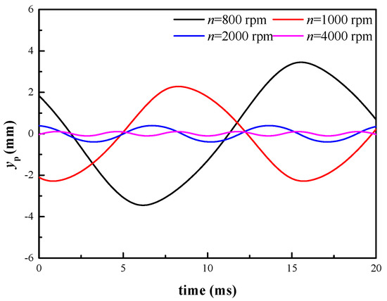
Figure 7.
Displacements of different valve spool rotation speeds when the proportional flow control valve port is fully open.
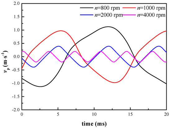
Figure 8.
Velocities of different valve spool rotation speeds when the proportional flow control valve port is fully open.

Figure 9.
Accelerations of different valve spool rotation speeds when the proportional flow control valve port is fully open.
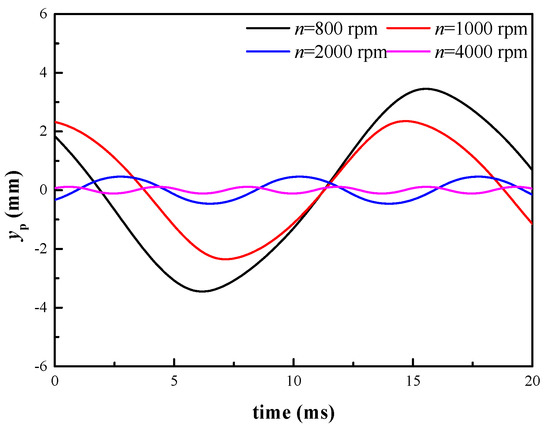
Figure 10.
Displacements of different valve spool rotation speeds when the supply pressure is 4 MPa.
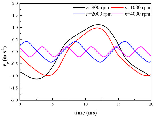
Figure 11.
Velocities of different valve spool rotation speeds when the supply pressure is 4 MPa.
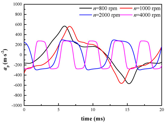
Figure 12.
Accelerations of different valve spool rotation speeds when the supply pressure is 4 MPa.
4.2. The Influence of Different Oil Supply Pressures on the Excitation Waveform
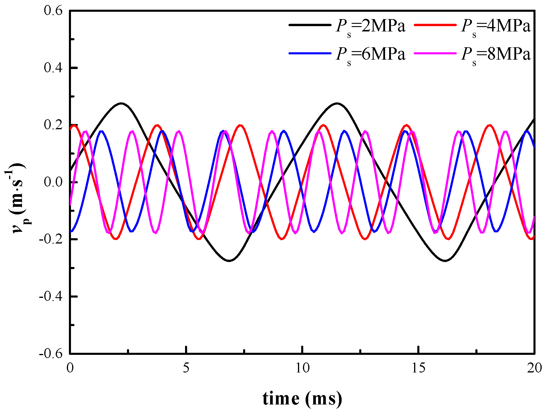
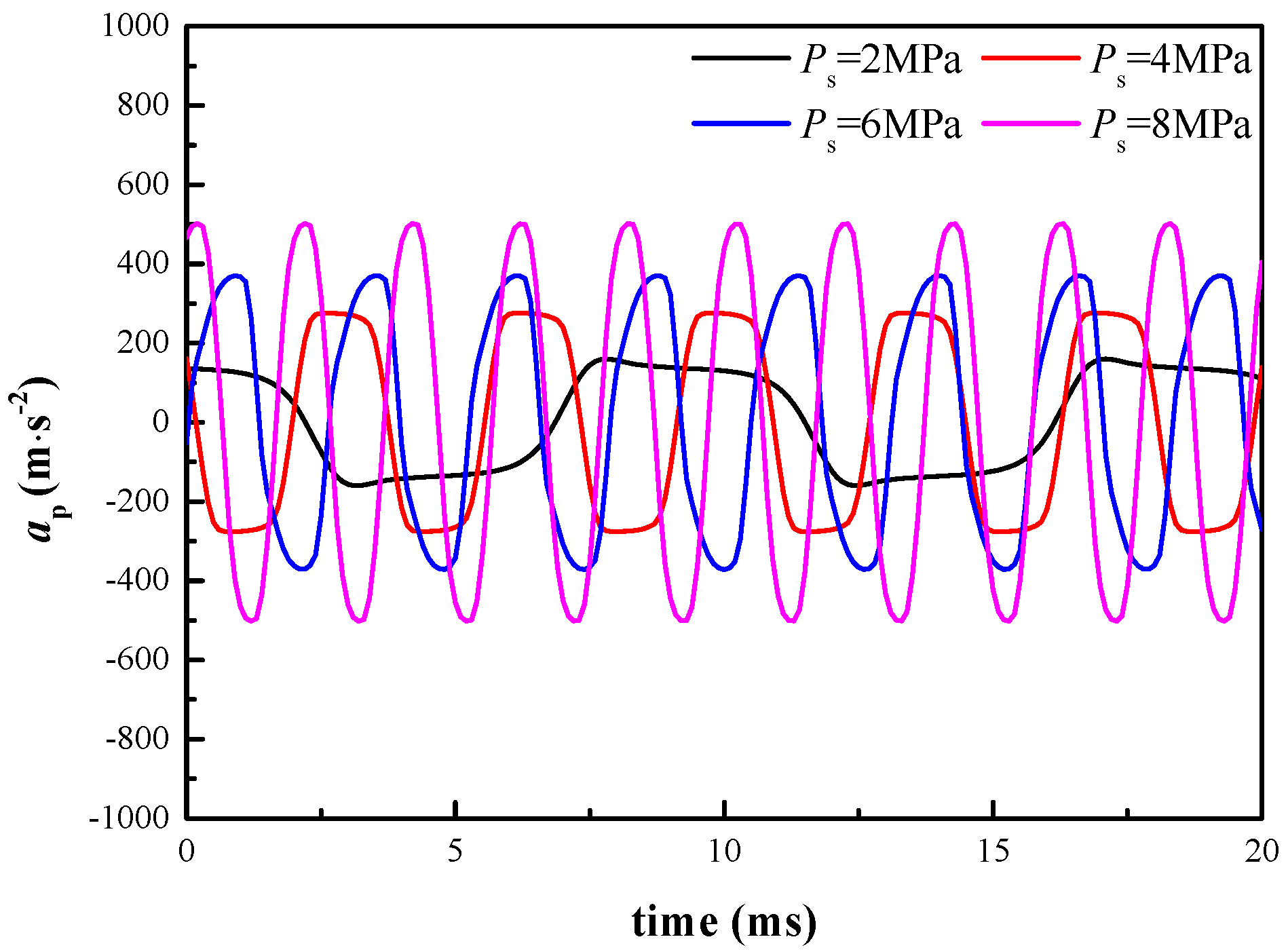
The relationships of the oil supply pressure with the displacement , velocity , acceleration , and reversing frequency curves are shown in Figure 13, Figure 14, Figure 15 and Figure 16. Figure 13 and Figure 14 indicate that as increases, the amplitude of and decreases gradually, and the amount of reduction in amplitude also decreases. Figure 15 and Figure 16 show that and increase as the oil supply pressure increases, because the motor branch and the rotary valve branch of the HCRV share the same hydraulic source. As the oil supply pressure increases, the flow into the motor branch also increases, causing the motor rotary speed to increase.
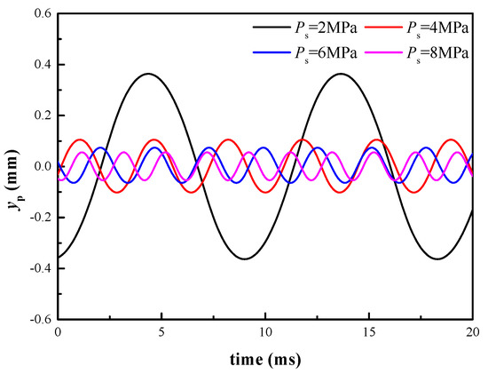
Figure 13.
Displacements of different supply pressures.

Figure 14.
Velocities of different supply pressures.

Figure 15.
Accelerations of different supply pressures.
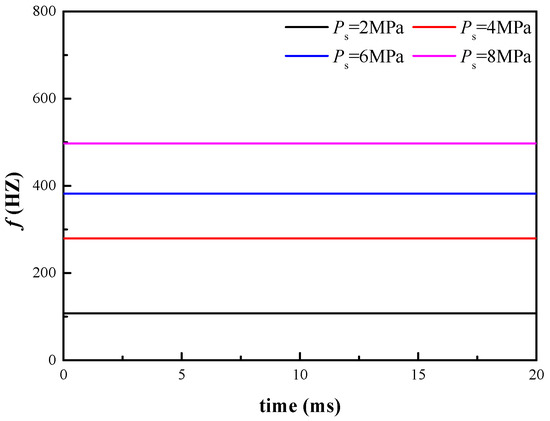
Figure 16.
Reversing frequencies s of different supply pressures.
4.3. The Influence of Different Orifice Numbers on the Excitation Waveform
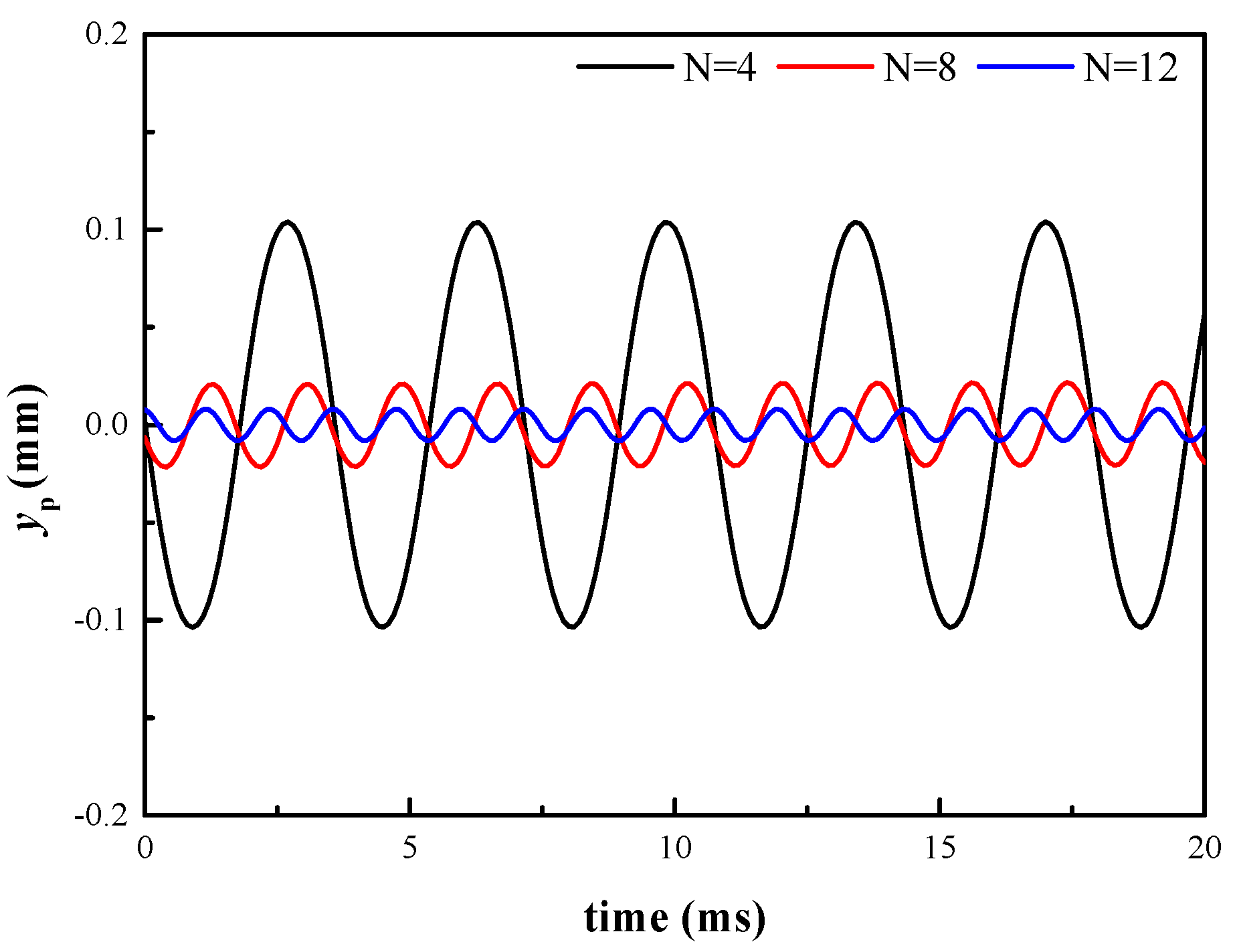
The relationships of the orifice number with the displacement , velocity , acceleration , and reversing frequency are shown in Figure 17, Figure 18, Figure 19 and Figure 20. Figure 17, Figure 18 and Figure 19 indicate that as increases, the amplitudes of , , and decrease gradually, and the amplitude reduction decreases too. Figure 20 shows that increases with , and the reversing frequency’s increase is proportional to the variation of the orifice number. According to the structure and working principle of the rotary valve, when the orifice number is doubled, the center angle corresponding to a single groove on the shoulder of the valve core becomes halved, and the peak value of the single orifice flow area is also halved. Therefore, in a vibration period, the peak value and change law of the orifice flow area remain unchanged. However, from formula , when the spool rotation speed is constant, is proportional to the orifice number (in other words, the change of the orifice number will cause another system parameter’s change–the reversing frequency), which means that the spool rotation speed increases.

Figure 17.
Displacements of different orifice numbers.
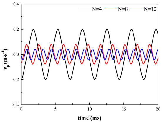
Figure 18.
Velocities of different orifice numbers.

Figure 19.
Accelerations of different orifice numbers.
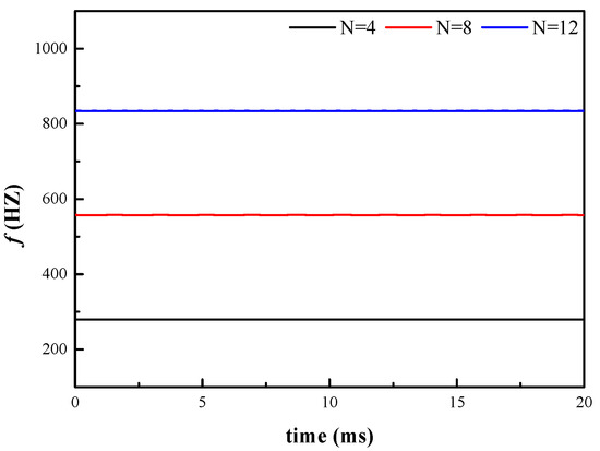
Figure 20.
Reversing frequencies of different orifice numbers.
4.4. The Influence of Different Orifice Shapes on the Excitation Waveform
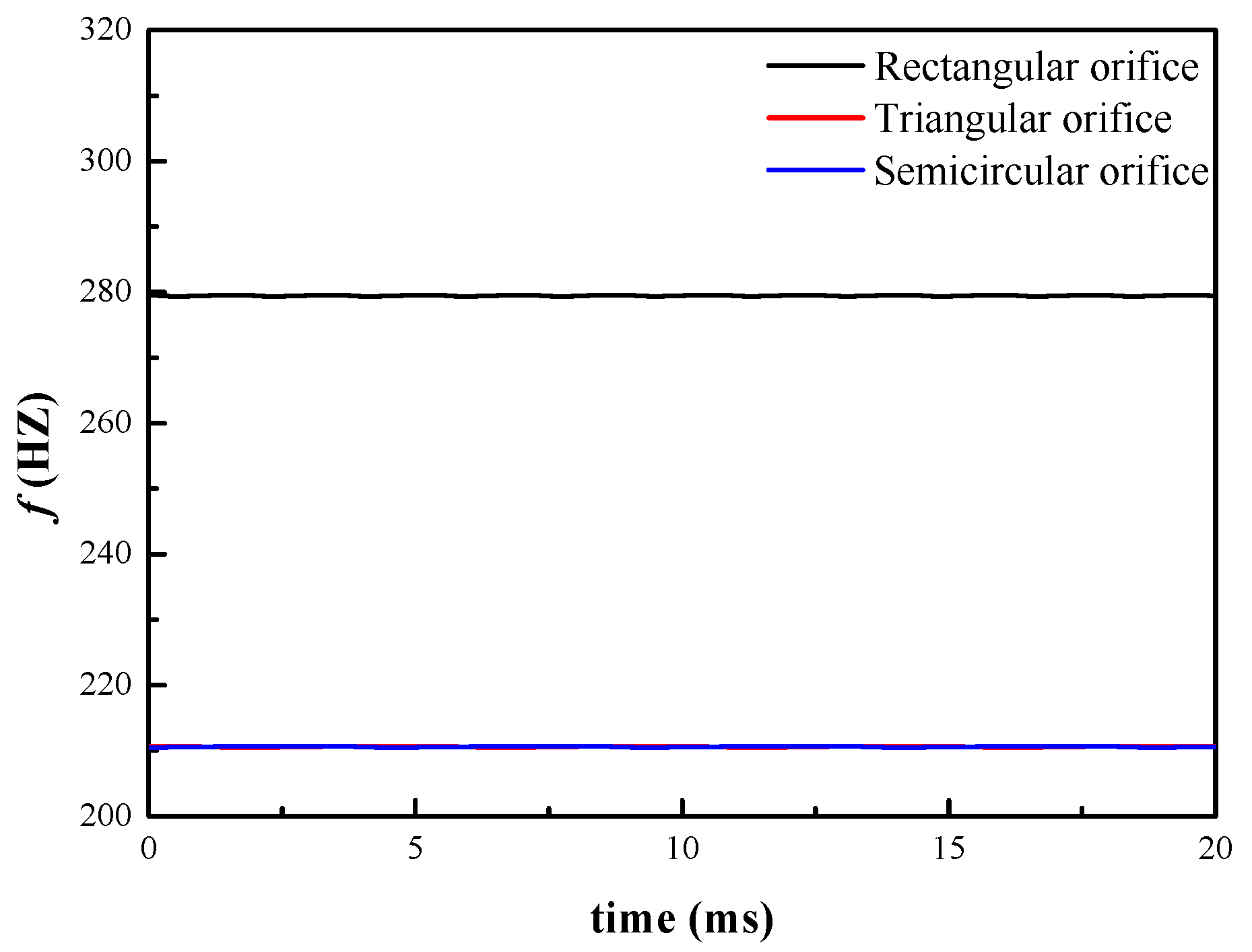
The relationships of the orifice shape with the displacement , velocity , acceleration , and reversing frequency are shown in Figure 21, Figure 22, Figure 23 and Figure 24. Figure 21 indicates that the amplitude of under the triangular and semicircular orifice is larger than that under the rectangular orifice, and the amplitude difference between the two orifice shapes is negligible. Figure 22 shows that the peak values of under the three orifice shapes are close to each other. Figure 23 indicates that the peak value of under the rectangular orifice is the maximum, and the peak value of under the semicircular orifice is the minimum. Figure 24 shows that under the rectangular orifice is greater than that under the triangular and semicircular orifices, and values under the triangular and semicircular orifices are not much different. From Equations (2), (4), and (6), when the supply pressure is constant, the flow under the rectangular orifice is the largest, which leads to the amplitudes of , , and under the rectangular orifice being larger than under the triangular and semicircular orifice. Moreover, in this case, the flow into the hydraulic motor branch also increases, which leads to a higher reversing frequency under the rectangular orifice.
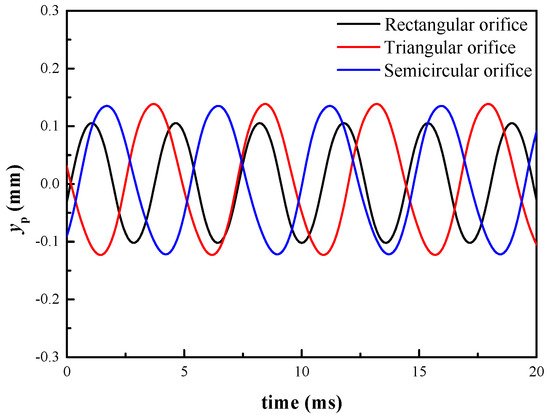
Figure 21.
Displacements of different orifice shapes.
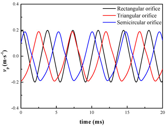
Figure 22.
Velocities of different orifice shapes.
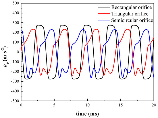
Figure 23.
Accelerations of different orifice shapes.

Figure 24.
Reversing frequencies of different orifice shapes.
4.5. The Influence of Different Orifice Axial Lengths on the Excitation Waveform
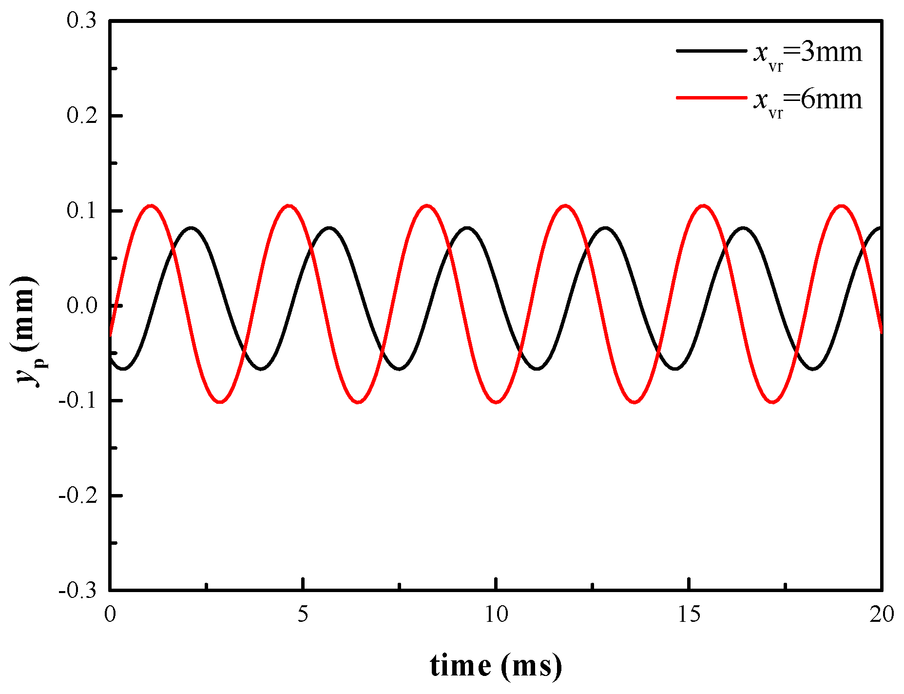
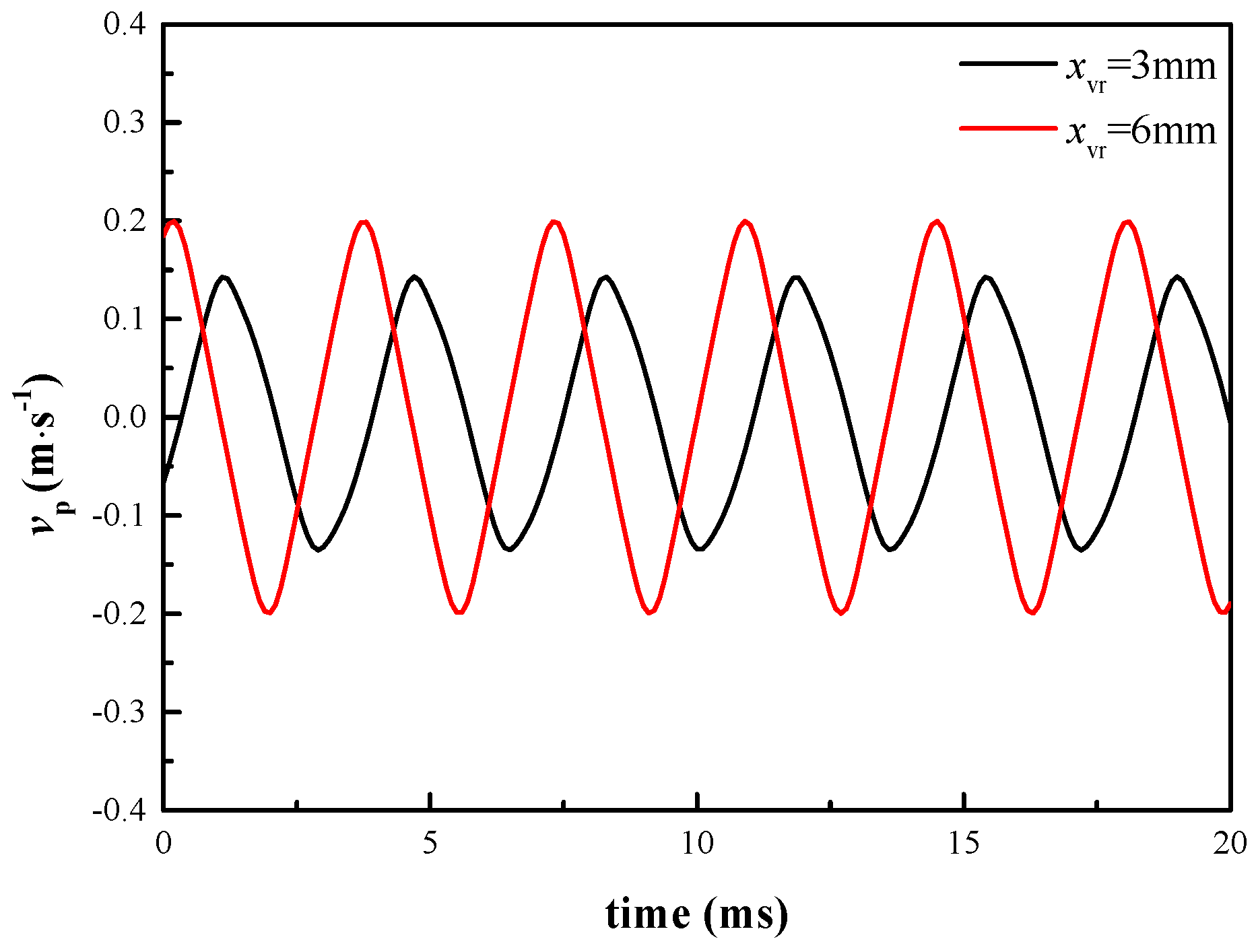
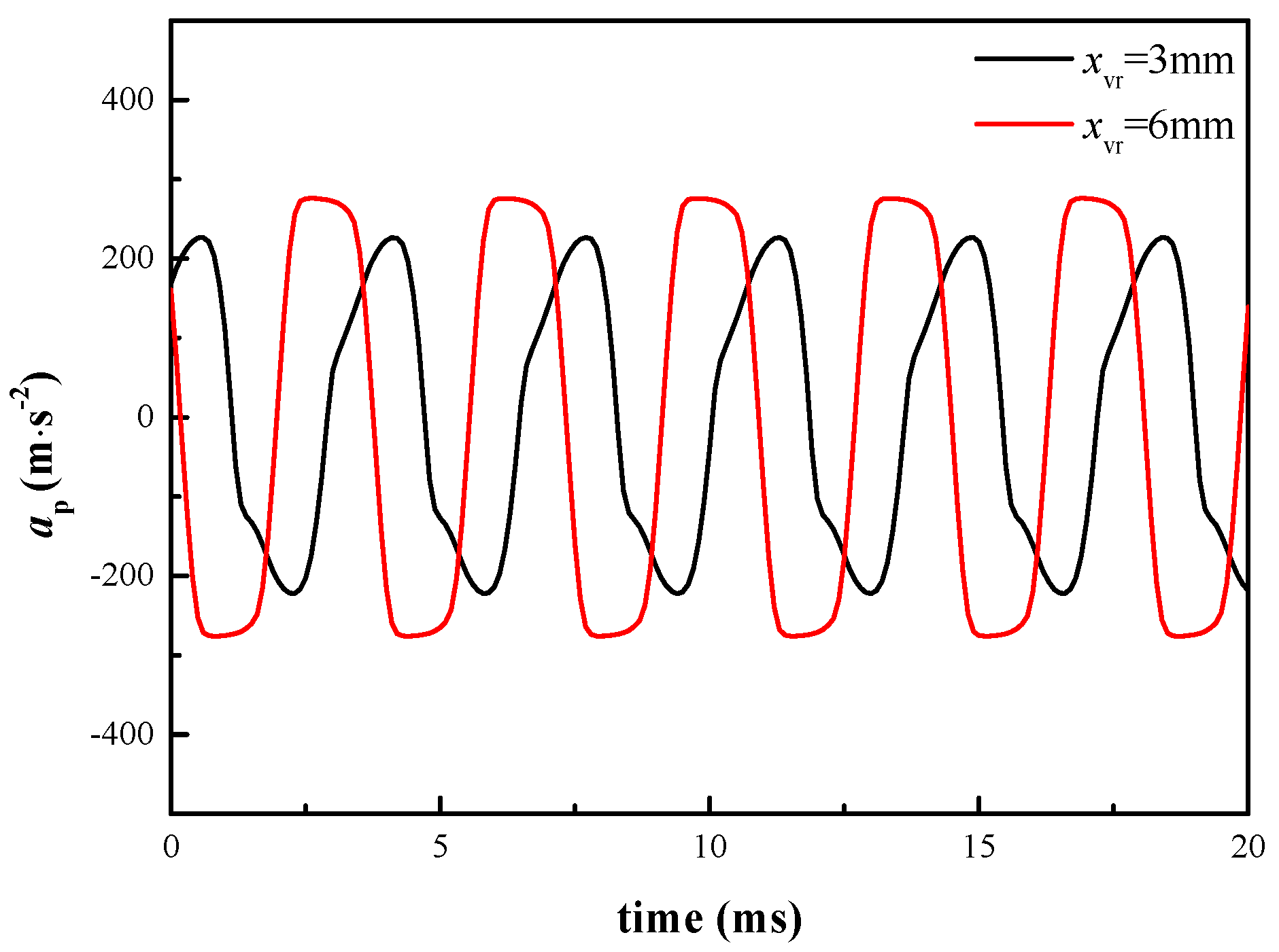
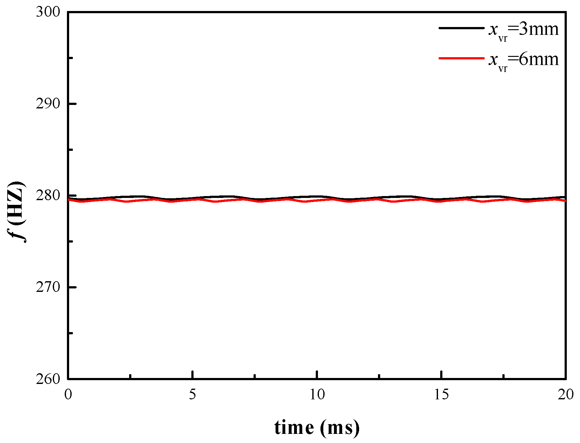
The relationships of the orifice axial length with the displacement , velocity , acceleration , and reversing frequency are shown in Figure 25, Figure 26, Figure 27 and Figure 28. It can be seen from Formula (3) that the greater the orifice axial length, the larger the flow area of the valve port. Therefore, when the spool rotation speed and oil supply pressure are constant, the amplitudes of , , and increase as the orifice axial length increases. Figure 28 shows that is not affected by the orifice axial length. In this case, the flow in the rotary valve branch increases as the orifice axial length increases, which leads the amplitudes of , , and to increase, while the flow in the hydraulic motor branch is almost unchanged.
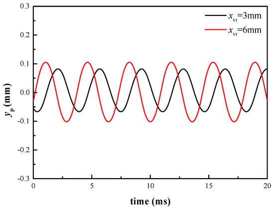
Figure 25.
Displacements of different orifice axial lengths.

Figure 26.
Velocities of different orifice axial lengths.
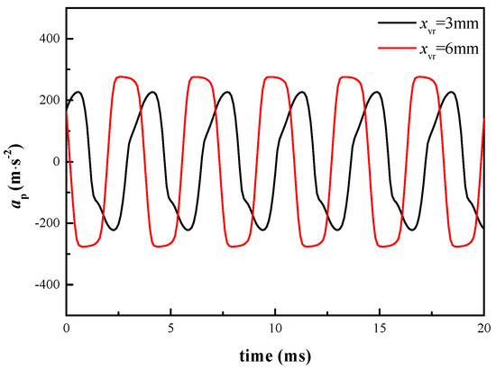
Figure 27.
Accelerations of different orifice axial lengths.
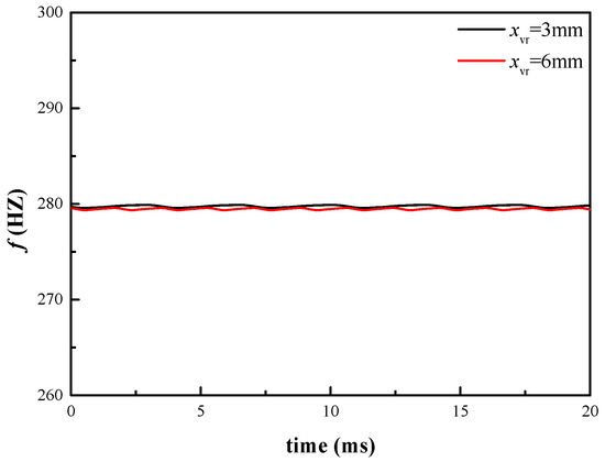
Figure 28.
Reversing frequencies of different orifice axial lengths.
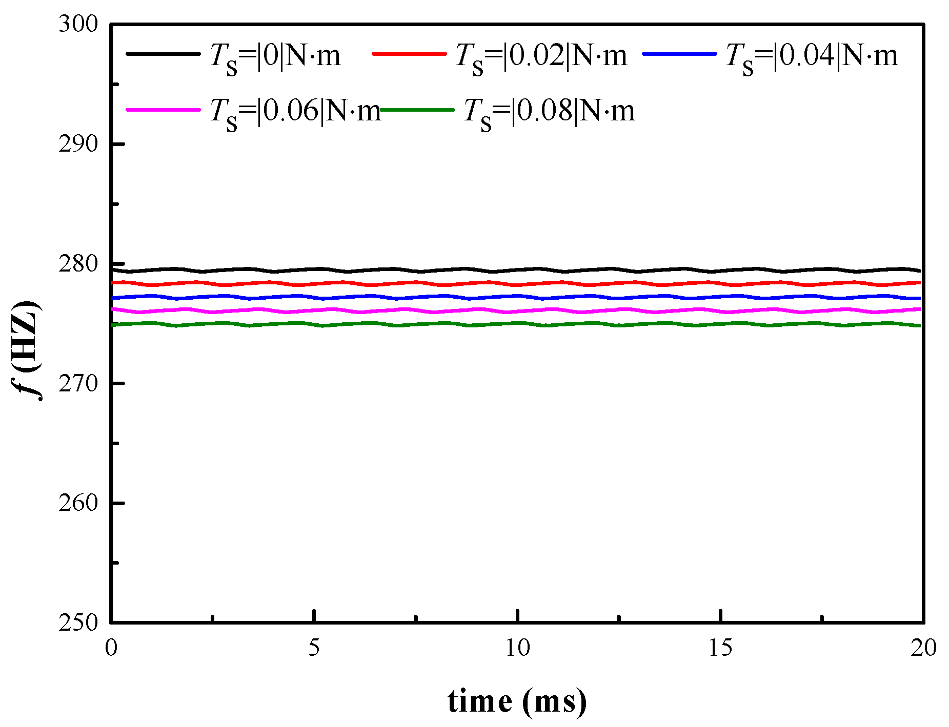
4.6. The Influence of Different Transient Flow Torques on the Excitation Waveform
The spool rotation process of the HCRV is affected by the transient hydraulic torque , and the direction of the transient flow torque is constantly changing. The relationships of the transient flow torque with the displacement , velocity , acceleration , and reversing frequency are shown in Figure 29, Figure 30, Figure 31 and Figure 32. The transient flow torque has little effect on the excitation waveform.
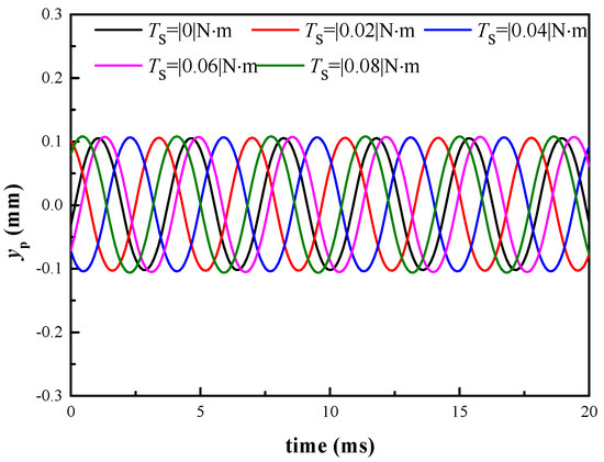
Figure 29.
Displacements of different transient flow torques.
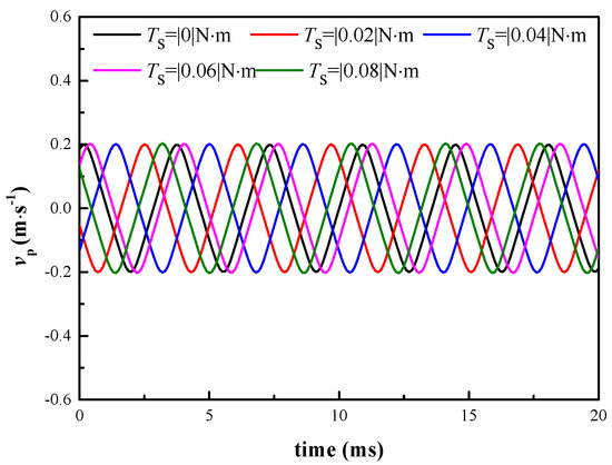
Figure 30.
Velocities of different transient flow torques.
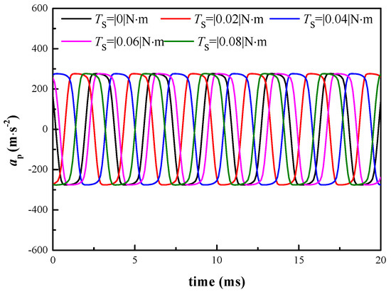
Figure 31.
Accelerations of different transient flow torques.
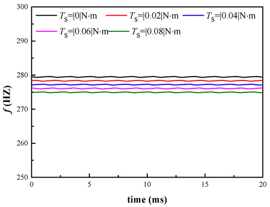
Figure 32.
Reversing frequencies of different transient flow torques.
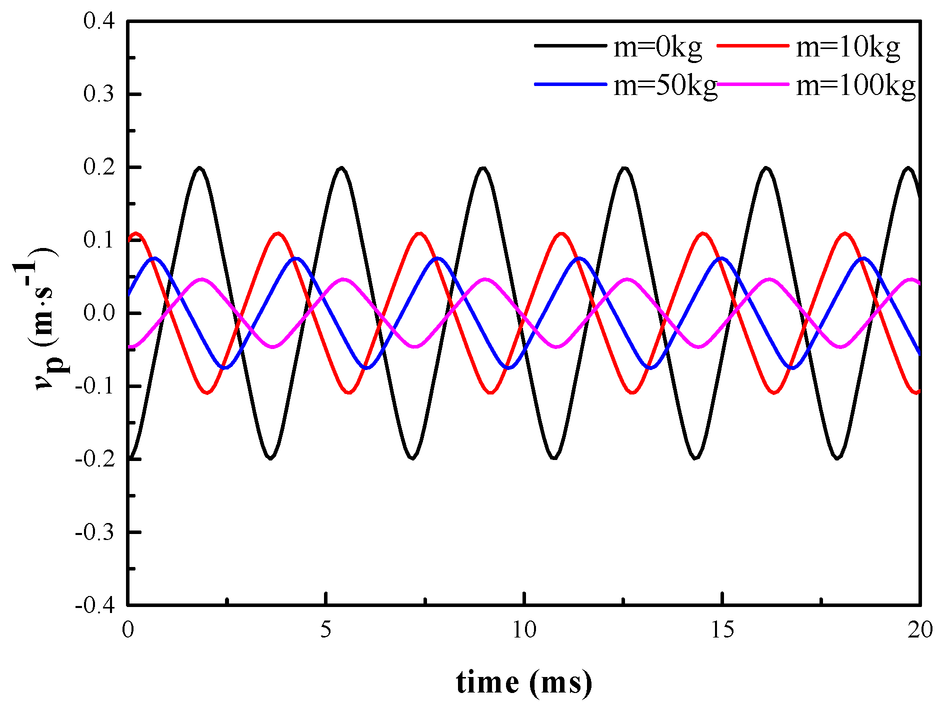
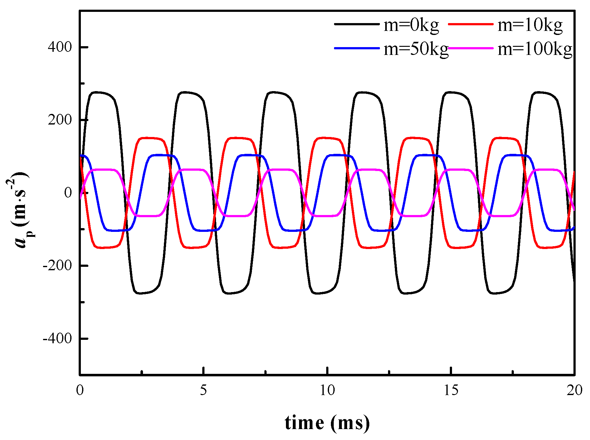
4.7. The Influence of Different Loads on the Excitation Waveform
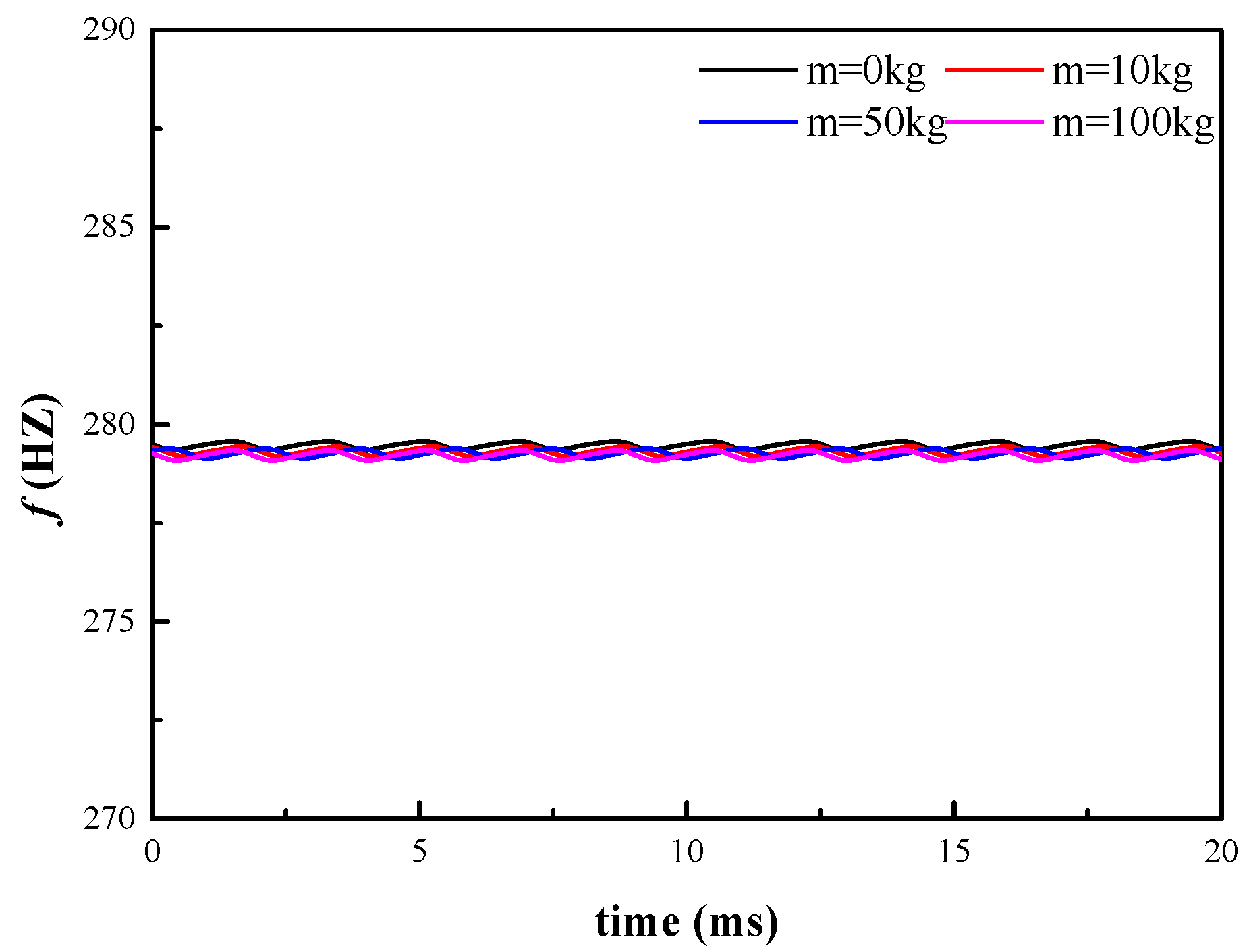
The relationships of the load with the displacement , velocity , acceleration , and reversing frequency are shown in Figure 33, Figure 34, Figure 35 and Figure 36. As the external load increases, the amplitude of and the peak values of and decrease. Figure 36 shows that the load has little effect on the reversing frequency , which reflects the load adaptability of the proposed system.
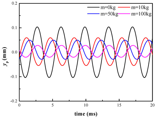
Figure 33.
Displacements of different loads.

Figure 34.
Velocities of different loads.
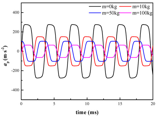
Figure 35.
Accelerations of different loads.

Figure 36.
Reversing frequencies of different loads.
5. Experimental Tests
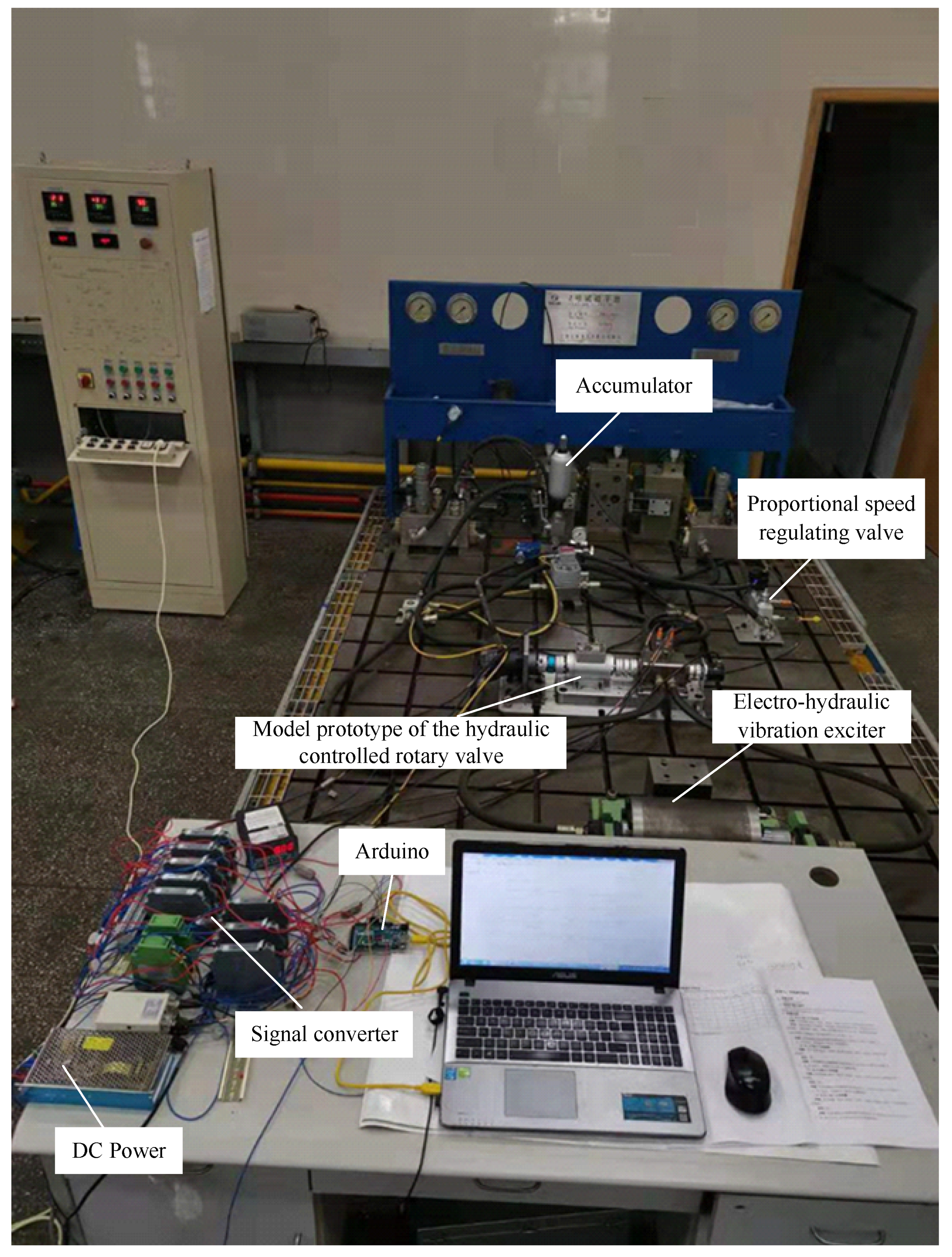
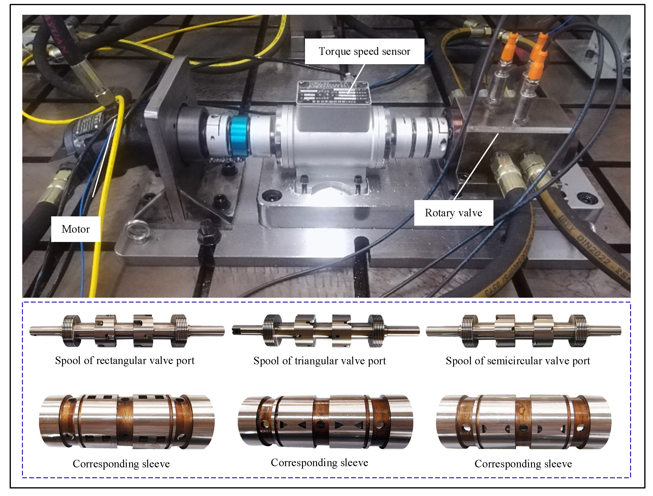
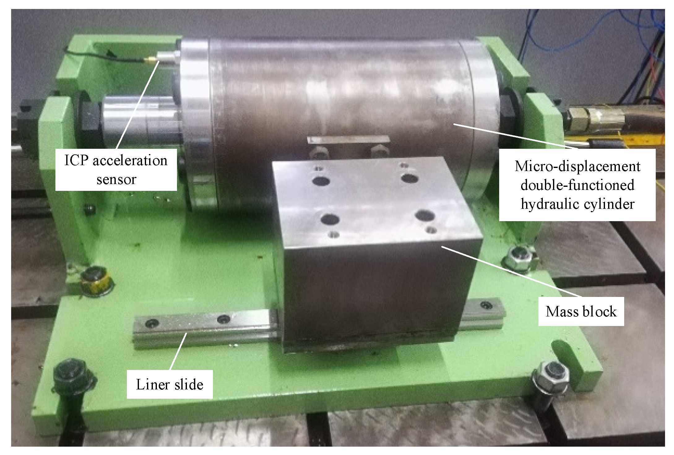
The experiments were conducted to verify the effectiveness of the proposed system scheme and the analysis results. In order to study more parameters’ relationships, the numerical simulation method was adopted, because the numerical simulation has the advantage of having more adjustable parameters and a lower cost than experiments. The experimental prototype bench of the HCRV excitation system is shown in Figure 37. The prototype model of the HCRV is shown in Figure 38, and is mainly composed of a hydraulic motor, a torque speed sensor, and a rotary valve. The electro–hydraulic vibration exciter is shown in Figure 39, and it includes a micro-displacement double functioned hydraulic cylinder, linear slide, and mass block. The hydraulic cylinder is equipped with an integrated circuits piezoelectric (ICP) acceleration sensor, which is used to measure the real time acceleration of the cylinder. The acquired acceleration signals are sent to the computer by the signal converter. The velocity and displacement waveforms of the HCRV excitation system are obtained by integrating and double integrating the acceleration. The specifications of the experimental setup are shown in Table 2.

Figure 37.
The experimental bench of the hydraulic controlled rotary valve excitation system.
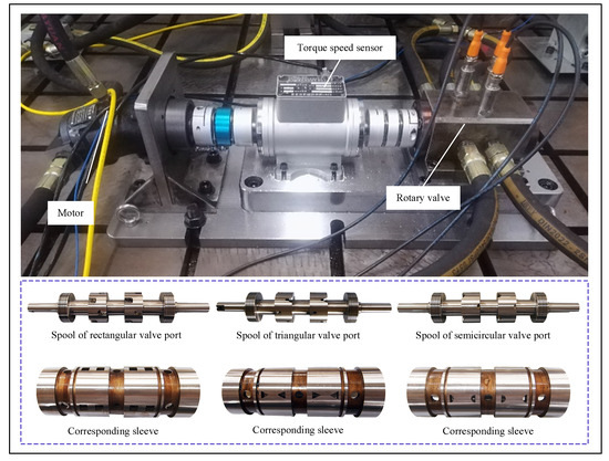
Figure 38.
Prototype model of the hydraulic controlled rotary valve.

Figure 39.
Electro-hydraulic vibration exciter.
Table 2.
The specifications of the experimental setup.
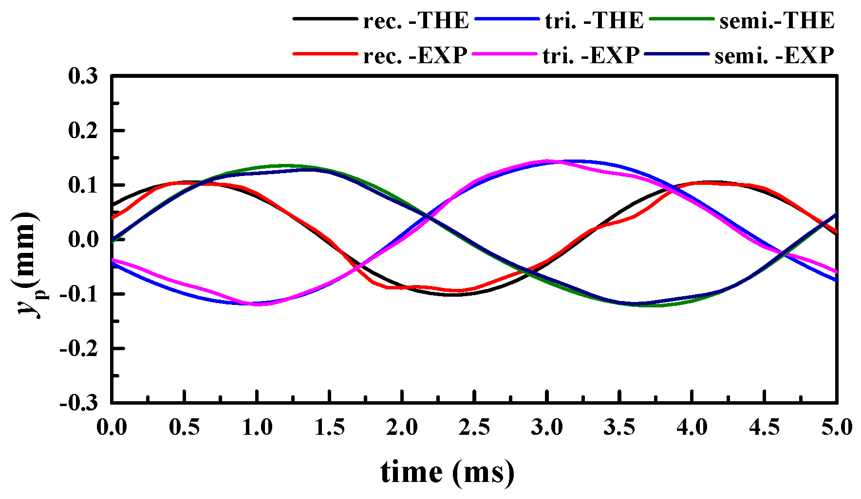
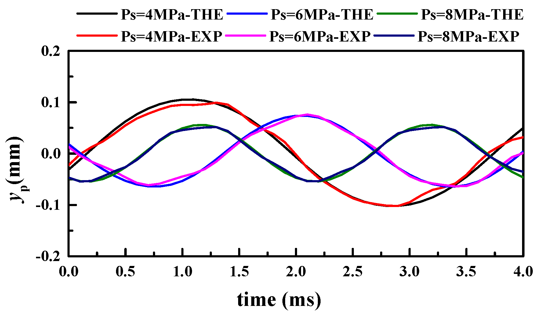
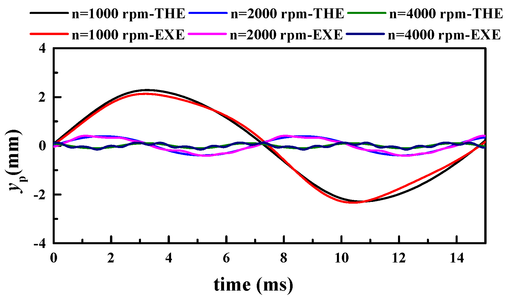
When the supply pressure is set to 4 MPa, experimental and theoretical curves of vibration waveforms of the HCRV excitation system with different orifice shapes are shown in Figure 40. The experimental and theoretical comparison of vibration waveforms of the HCRV excitation system at the rectangular valve orifice under different supply pressures is shown in Figure 41. The experimental and theoretical comparison of vibration waveforms at the rectangular valve orifice under different spool rotation speeds is shown in Figure 42. Meanwhile, the different mean square errors (MSE) between theoretical and experimental curves are given in Figure 40, Figure 41 and Figure 42. Comparing the experimental and theoretical curves under different conditions, it can be found that the experimental curve and theoretical curve are similar to each other. The comparison demonstrates the effectiveness of the proposed system scheme and the theoretical results.

Figure 40.
Vibration waveforms of different orifice shapes (MSErec. = 9.21 × 10⁻⁴, MSEtri. = 8.67 × 10⁻⁴, MSEtri. = 2.71 × 10⁻⁴).

Figure 41.
Vibration waveforms of different oil supply pressures (MSE4MPa = 5.33 × 10⁻⁴, MSE6MPa = 4.12 × 10⁻⁴, MSE8MPa = 2.24 × 10⁻⁴).

Figure 42.
Vibration waveforms of different spool rotation speeds (MSE1000rpm = 1.57 × 10⁻³, MSE2000rpm = 1.87 × 10⁻⁴, MSE4000rpm = 1.69 × 10⁻⁴).
6. Conclusions
In this paper, a novel full HCRV excitation system was proposed and a corresponding simulation model was developed. Many parameters affect the system’s output vibration waveform, such as the valve spool rotation speed, orifice number, supply pressure, orifice shape, orifice axial length, transient flow torque, and load, to mention but a few. The effects of the main parameters were analyzed, and the coupling relationship of parameters was revealed. Finally, experimental studies were conducted to show the effectiveness of the proposed system scheme and the analysis results.
- The proposed HCRV excitation system can achieve a high reversing frequency (300 HZ) and integrate the system more tightly. It is appropriate for electro-hydraulic excitation systems.
- The spool rotation speed is positive relative to the proportional flow control valve opening and the oil supply pressure.
- Parameters such as the spool rotation speed, oil supply pressure, orifice number, orifice axial length, and load have relatively obvious effects on the vibration waveform, while the orifice shape and transient flow torque have little influence on the waveform.
- The supply pressure, orifice number, and orifice shape have greater effects on the vibration reversing frequency, and the reversing frequency is proportional to the variation of the orifice number. The orifice axial length, transient flow torque, and load have almost no effects on the vibration reversing frequency.
- The external load has little effect on the vibration reversing frequency, which reflects the load adaptability of the HCRV excitation system.
Future work will be focused on the improvement of the proposed system and its parameters’ optimization.
Author Contributions
Writing—Original Draft Preparation, W.L.; Writing—Review & Editing, W.L., G.G. and Y.Z.; Software, W.L., J.L.; Validation, W.L.; Project Administration, G.G.; Investigation, Y.C., F.W.; Supervision, G.G., Y.Z. All authors have read and agreed to the published version of the manuscript.
Funding
This research was funded by the National Natural Science Foundation of China (Grant No. 51675472) and the National Key R&D Program of China (Grant Nos. 2017YFB1302600, 2017YFB1302602 and 2017YFB1302604), China.
Acknowledgments
The authors acknowledge Yuanchao Wang for his assistance in developing and maintaining the test bench.
Conflicts of Interest
The authors declare no conflict of interest. The funders had no role in the design of the study; in the collection, analyses, or interpretation of data; in the writing of the manuscript, and in the decision to publish the results.
References
- Kim, J.W.; Xuan, D.J.; Kim, Y.-B. Design of a forced control system for a dynamic road simulator using QFT. Int. J. Automot. Technol. 2008, 9, 37–43. [Google Scholar] [CrossRef]
- Chen, C.; Ricles, J.M. Improving the inverse compensation method for real-time hybrid simulation through a dual compensation scheme. Earthq. Eng. Struct. Dyn. 2009, 38, 1237–1255. [Google Scholar] [CrossRef]
- Rosas, D.I.; Velazquez, V.K.; Olivares, F.L.; Camacho, T.A.; Williams, I. Methodology to assess quality of estimated disturbances in active disturbance rejection control structure for mechanical system. ISA Trans. 2017, 70, 238–247. [Google Scholar] [CrossRef] [PubMed]
- Severn, R.T. The development of shaking tables—A historical note. Earthq. Eng. Struct. Dyn. 2011, 40, 195–213. [Google Scholar] [CrossRef]
- Stroud, R.C.; Hamma, G.A.; Underwood, M.A. A review of multi-axis/multi-exciter vibration technology. Sound Vib. 1996, 30, 20–27. [Google Scholar]
- Li, Q.P. Research on the Key Technologies of Direct Drive Servo Valve. Ph.D. Thesis, Zhejiang University, Hangzhou, China, 2005. [Google Scholar]
- Nascutiu, L. Voice Coil Actuator for hydraulic servo valves with high transient performances. In Proceedings of the 2006 IEEE International Conference on Automation, Quality and Testing, Robotics, Cluj-Napoca, Romania, 25–28 May 2006; pp. 185–190. [Google Scholar]
- Sallas, J.J. Low Inertia Servo Valve. U.S. Patent 5,467,800, 21 November 1995. [Google Scholar]
- Leonard, M.B. Rotary Servo Valve. U.S. Patent 5,954,093, 21 September 1999. [Google Scholar]
- David, G.; Ed, W.; Chris, W. Rotary Disc Valve. UK Patent GB 2,398,856 A, 24 August 2004. [Google Scholar]
- Lu, J.-x.; Li, S.-L.; Jiao, Z.X. A limited-angle rotating of electro-hydraulic servo-valve. Hydraul. Pneum. Seals 2005, 4, 40–42. [Google Scholar]
- Zhang, G.Q.; Chang, Y.D. Bidirectional polarized proportional electromagnet and its static and dynamic characteristics. Explos.-Proof Electr. Appar. 1989, 4, 28–32. [Google Scholar]
- Ruan, J.; Pei, X.; Li, S. A two-dimensional electrohydraulic digital directional valve. J. Mech. Eng. 2000, 36, 86–89. [Google Scholar] [CrossRef]
- Ruan, J.; Burton, R.T. An electrohydraulic vibration exciter using a two-dimensional valve. Proc. Inst. Mech. Eng. Part I J. Syst. Control. Eng. 2008, 223, 135–147. [Google Scholar] [CrossRef]
- Ruan, J. Electrohydraulic vibration exciter controlled by 2D valve. Chin. J. Mech. Eng. 2009, 45, 125. [Google Scholar] [CrossRef]
- Haidegger, T.; Kovács, L.; Preitl, S. Controller design solutions for long distance telesurgical applications. Int. J. Artif. Intell. 2011, 6, 48–71. [Google Scholar]
- Precup, R.-E.; Tomescu, M.-L. Stable fuzzy logic control of a general class of chaotic systems. Neural Comput. Appl. 2014, 26, 541–550. [Google Scholar] [CrossRef]
- Han, D.; Gong, G.F.; Liu, Y. New electro-hydraulic exciter based on different spools. J. Zhejiang Univ. (Eng. Sci.) 2014, 48, 757–763. [Google Scholar]
- Li, W.; Gong, G.; Wang, Y.; Zhang, Y.; Chen, Y. Modeling and analysis of hydraulic controlled rotary valve excitation system. In Proceedings of the 2019 IEEE/ASME International Conference on Advanced Intelligent Mechatronics, Hong Kong, China, 8–12 July 2019; pp. 340–345. [Google Scholar]
- Gong, G.F.; Wang, Y.C.; Li, W.J. An Integrated Machine of the Hydraulic Motor Coupled to the Rotary Valve. China Patent ZL 201810329041.3, 28 September 2018. [Google Scholar]
- Wang, H. Research on the Key Technologies of High Speed Rotary Directional Control Valve. Ph.D. Thesis, Zhejiang University, Hangzhou, China, 2016. [Google Scholar]
- Hou, Y.J.; Yuan, Q.H. Simulation analysis of the three-cylinder reciprocating pump hydraulic system controlled by rotary valve. China Petroleum Mach. 2011, 39, 15–18. [Google Scholar]
- Wu, W.R.; Huang, Q.; Wu, W.W. Simulation of high frequency excitation rotary valve with two degrees of freedom based on AMESim. World Sci.-Tech. R D 2016, 38, 1228–1233. [Google Scholar]


© 2020 by the authors. Licensee MDPI, Basel, Switzerland. This article is an open access article distributed under the terms and conditions of the Creative Commons Attribution (CC BY) license (http://creativecommons.org/licenses/by/4.0/).