Validating CFD Predictions of Flow over an Escarpment Using Ground-Based and Airborne Measurement Devices

Abstract

Micrometeorological observations from a tower, an eddy-covariance (EC) station and an unmanned aircraft system (UAS) at the WINSENT test-site are used to validate a computational fluid dynamics (CFD) model, driven by a mesoscale model. The observation site is characterised by a forested escarpment in a complex terrain. A two-day measurement campaign with a flow almost perpendicular to the escarpment is analysed. The first day is dominated by high wind speeds, while, on the second one, calm wind conditions are present. Despite some minor differences, the flow structure, analysed in terms of horizontal wind speeds, wind direction and inclination angles shows similarities for both days. A real-time strategy is used for the CFD validation with the UAS measurement, where the model follows spatially and temporally the aircraft. This strategy has proved to be successful. Stability indices such as the potential temperature and the bulk Richardson number are calculated to diagnose atmospheric boundary layer (ABL) characteristics up to the highest flight level. The calculated bulk Richardson values indicate a dynamically unstable region behind the escarpment and near the ground for both days. At higher altitudes, the ABL is returning to a near neutral state. The same characteristics are found in the model but only for the first day. The second day, where shear instabilities are more dominant, is not well simulated. UAS proves its great value for sensing the flow over complex terrains at high altitudes and we demonstrate the usefulness of UAS for validating and improving models.

1. Introduction

To achieve the objective of making the European Union climate-neutral by 2050, it will be necessary to maximize the deployment of renewable energy in the years to come [1]. The clean energy transition involves encouraging high levels of renewable energy penetrations. Harvesting power from wind power is one of the fastest-growing renewable energy methods. To meet the climate-neutral target, more wind energy capacity will be installed in the coming years. Independent of the exact number of new installations, most of them will be onshore [2].

A wind energy project includes site investigation, resource assessment, environmental impact assessment, technical and administrative procedures with local communities and, finally, construction work. The site investigation and resource assessment phases need accurate and reliable models for predicting the wind flow. During the last two decades, linear flow models, mainly based on the Jackson–Hunt theory [3], were extensively used in the wind industry for wind resource assessment and micro-siting. These models are, however, inaccurate for wind speed prediction in very complex terrain, which led to the use of computational fluid dynamics (CFD), capable of modelling the wind flow in details around specific orographic features. The spatial and temporal variability of the atmospheric boundary layer (ABL) makes the prediction of the wind flow by models one of the main challenges, especially in complex terrain. The commercial CFD software for wind resource assessment uses logarithmic wind profile and tunes parameters from the Monin–Obukhov similarity theory [4] to calculate annual energy prediction for site assessment. The logarithmic wind profiles are not site specific and don’t have micro meteorological information of wind at the particular site. This is a major error source for the calculation of annual energy production. Hence, the variability of the atmosphere should be considered at the mesoscale. Only weather forecast models, driven by global models, can capture the dynamic processes of the atmosphere [5]. Today’s mesoscale models are used increasingly for wind-energy applications with efforts in improving surface winds in complex terrain [6,7]. However, it has been observed that numerical noise is appearing with increasing terrain complexity [8]. A remedy is to use the data from mesoscale models of a given region as a realistic boundary condition for a more detailed microscale modelling. That way, the wind characteristics can be determined at a high resolution in the area of interest. This approach is referred in the literature as mesoscale-microscale modelling and have been successfully used in different domains. For instance, the improved predictability of pollutants such as NO${}_x$ and NO${}_2$ in urban areas by coupling a mesoscale model with a CFD model has been demonstrated in recent studies [9,10]. For wind assessment studies, the performance of coupled simulations is more and more recognized and has been extended. Even in the industry, it showed an improvement of wind power forecasting [11].

All methods and models should be validated, ideally with in-situ and/or remote sensing measurements. The need for field campaigns to provide data for model validation in complex terrain has led to the funding of several projects over the last few years. Examples are the Kassel Experiment in Germany [12], the Alaiz Experiment in Spain [13], the double-ridge Perdigao in Portugal [14] or the Wind Forecast Improvement Project (WFIP2) in the U.S [15], all aiming at improving the understanding of physical processes and wind forecasts in complex terrain. Traditional in-situ platforms for atmospheric measurements are towers installed at a certain location. The vertical information is provided by instruments installed at several discrete levels. They can provide continuous recording of the investigated variables over long time periods. To follow the growth of wind turbine sizes, the meteorological tower should ideally become taller and have the same height as the wind turbines, making their installation technically complicated and more expensive. These limitations have led to the use of lidar (light detection and ranging) technologies for wind measurements. However, in complex environments, the spatial heterogeneity and transient features introduced by the terrain can lead to difficulties in interpreting the line of sight wind speed and reconstructing the wind field [16]. For instance, the central goal of the International Energy Agency Wind Task 32 community is developing frameworks for the deployment and use of wind lidars in complex flow. One promising approach is the use of two or more lidars to reconstruct the flow field in a complex terrain. Limitations of this approach are mainly the high costs and the uncertainties [17]. Other emerging techniques for wind-energy applications are flying platforms. Small unmanned aircraft systems (UAS) have become frequently used platforms for ABL research. They have the advantage of being versatile, even in highly complex terrain and the necessary infrastructure is small compared to masts and active remote sensing techniques. They can fly in the close vicinity of a wind turbine, even at very low altitudes, where the main vertical and horizontal inhomogeneities are occurring. The capability of UAS for turbulence characterization and providing high spatial-temporal sampling frequencies has been demonstrated in research works over the last several years. The use of these systems contributed to a better characterisation and understanding in aerosol formations [18,19], storm developments [20], atmospheric research [21,22,23], or for wind energy purposes [24,25].

In the research project WINSENT (Wind Science and Engineering Test Site in Complex Terrain), a field test-site is being built on the Swabian Alb in Southern Germany [26]. It will be the first wind energy test-site of this size in complex terrain. The first phase of the WINSENT project investigates the local wind flow at the test-site using different measurement equipments and simulation models. During the second stage, two wind turbines with a nominal output of around 750 kW will be installed next to the escarpment. The effect of the topography on the wind-turbines performances, wakes, and material fatigue will be studied both experimentally and numerically [27,28]. The on-site instruments consist of permanently installed towers equipped with ultrasonic anemometers and eddy-covariance (EC) micro-meteorological stations. Additionally, the multipurpose airborne sensor carrier MASC [29] and several lidars [30] carry out measurements over and downstream of the escarpment during different measurement campaigns. All of the equipment is going to provide new datasets to evaluate and validate the numerical models. In the framework of the WINSENT project, a numerical study is conducted with models, with a different range of scales such as the Weather Research and Forecasting (WRF) model [31], the Open Source Field Operation and Manipulation (OpenFOAM) software [32], and the solver FlOWer [33].

In the present study, a numerical and experimental investigation of the flow at the WINSENT test-site is presented. Two flight measurement campaigns, which took place over two days in September 2018, are analysed. The first day is dominated by high wind speeds while the conditions on the second day are calmer. Measurements by the MASC, along with a meteorological tower and an EC station are used for the evaluation of our model. A real-time strategy is adopted for the comparison of the numerical results with the MASC measurements. The performance of our methodology is presented in this study as follows: in Section 2, the numerical tools are presented, while, in Section 3, the test-site along with the measurement devices are described. Section 4 discusses the numerical and experimental results from the measurement campaigns together with a stability analysis and finally a conclusion with outlooks is given in Section 5.

2. Methods

2.1. Numerical Model

In the current study, the wind flow is simulated using the software OpenFOAM v6. An unsteady Reynolds Averaged Navier–Stokes (URANS) approach, necessary for the investigation of non-stationary flow features, was considered [34,35]. The governing equations for mass, momentum, and potential temperature, under the Boussinesq approximation, are written relative to a hydrostatic state (index h) in a Cartesian coordinate system as:

$$\frac{\partial }{\partial t}\left({\rho }_h\right)+\frac{\partial }{\partial x_j}\left({\rho }_h{u}_j\right)=0$$

(1)

$$\frac{\partial }{\partial t}\left({\rho }_h{u}_i\right)+\frac{\partial }{\partial x_j}\left({\rho }_h{u}_i{u}_j\right)=-\frac{\partial p^{*}}{\partial x_i}+\frac{\partial }{\partial x_j}\left[(\mu +{\mu }_t)\left(\frac{\partial u_i}{\partial x_j}+\frac{\partial u_j}{\partial x_i}-\frac{2}{3}k{\delta }_{ij}\right)\right]-{\rho }_h{g}_i\frac{\theta -{\theta }_h}{{\theta }_h}+F_{Ci}+F_{Di}$$

(2)

$$\begin{array}{cc}\hfill \frac{\partial }{\partial t}\left({\rho }_h\theta \right)+\frac{\partial }{\partial x_i}\left({\rho }_h{u}_i\theta \right)& =\frac{\partial }{\partial x_i}\left[(\mu +\frac{{\mu }_t}{{\sigma }_h})\left(\frac{\partial \theta }{\partial x_i}\right)\right]\hfill \end{array}$$

(3)

where $u_i(i=1,2,3)$ are the velocity components in a Cartesian framework (x, y, z, where z is aligned with gravity), p and $\theta$ are the pressure perturbation from the hydrostatic reference state and potential temperature, $\mu$ and ${\mu }_t$ are the dynamic molecular and turbulent eddy viscosities, $g_i$ is the gravitational acceleration term, and ${\sigma }_h$ is the turbulent Prandtl number. $F_{Ci}$ and $F_{Di}$ are the source term representing the Coriolis and the drag force exerted by the forest on the wind flow, respectively. The hydrostatic fluid density ${\rho }_h$ is defined in a hydrostatic reference state (subscript 0) as a function of the hydrostatic pressure $p_h$ and the temperature $T_h$ as:

$$\begin{array}{cc}\hfill {\rho }_h& =\frac{p_h}{R_d{T}_h}\hfill \end{array}$$

(4)

$$\begin{array}{cc}\hfill T_h& =T_0\sqrt{1-\frac{2Agz}{R_d{T}_0^2}}\hfill \end{array}$$

(5)

$$\begin{array}{cc}\hfill p_h& =p_0\exp \left(\frac{-T_0}{A}\left(1-\sqrt{1-\frac{2Agz}{R_d{T}_0^2}}\right)\right)\hfill \end{array}$$

(6)

where $p_0$ is the constant reference pressure set to 1000 hPa, $T_0$ is the reference temperature equal to 288.5 K, $A=50$ K, and $R_d=287.05$ J kg${}^{-1}$ K${}^{-1}$ [36,37]. The Sogachev $k-ϵ$ model is used for the turbulence closure [38]. Additionally, source terms in the turbulent kinetic energy and turbulence dissipation rate equations, using the constants proposed by [39] were added in order to take into account for the drag effect of vegetation on the flow.

2.2. Computational Set Up and Mesoscale Forcing

The simulations are conducted on a domain of 10 × 10 × 2.5 km${}^3$, centered in the escarpment. The spatial resolution consists of 10 m increments in the horizontal directions and the vertical discretization has values between 1.8 m at the ground and 80 m at the top of the domain. The terrain data are based on the digital height model from the Baden–Württemberg Authorities for Spatial Information and Rural Development (LGL) with a spatial resolution of 5 m. In addition, the digitized landscape model from LGL was utilized to describe the land cover on the Earth’s surface. Three classes of land uses were retained for this study: urban, ground, and forest (Figure 1b). In this paper, a deciduous forest with a height of 20 m is considered for the forest patch. The urban and the ground classes were assigned values of 0.50 m and 0.02 m for the aerodynamic roughness length.

The mesoscale flow is simulated using WRF with five nested domains. WRF uses the European Centre for Medium-Range Weather Forecasts analysis data as initial and boundary conditions. The innermost nest has a horizontal grid size of 150 m, a vertical grid size of 15 m close to the ground and is run in a large eddy simulation mode. A one-way nesting method was used for the coupling of WRF and OpenFOAM: the innermost nest provides boundary conditions to the microscale model. Border data include the velocity components, pressure and temperature at 1-minute intervals. The WRF model provides also the heat flux at the ground. No special temporal and spatial interpolation has been applied as the mesoscale model is considered fine enough near the ground.

3. Test Site and Measurements

3.1. Test Site

The field measurements were made at the WINSENT test-site, built on the Swabian Alb in Southern Germany. The main feature of the site is a sloping escarpment up to 200 m in height with respect to the valley (see Figure 1a). The escarpment is characterized by a very steep slope of around 30$°$ from the Northwest and a more gradual slope at around 15$°$ further west. A dense vegetation with a tree height between 15 and 25 m is covering the escarpment. To the east of the escarpment, the ground is essentially flat and under agricultural use. The windrose (Figure 1c) measured on a height of 86 m at the test-site shows winds blowing predominantly from the west, and therefore perpendicular to the escarpment, most of the year.

3.2. Measurements

Measurements took place on 21 and 22 September 2018. Cup anemometers sampling at 20 Hz are mounted on the tower (48.6652$°$ latitude, 9.8347$°$ longitude) along with hygrothermographs, wind vanes, and barometers at various heights between 3 and 100 m (

Table 1. Overview of instruments.

Instrument, Mark	Location: Height above Ground Level (a.g.l.)
Cup anemometer, Thies	10, 45, 59, 72, 86, 100
Hygrothermograph, Thies	3, 25, 45, 72, 96
Barometric Pressure Transducer, Setra	3, 96
Wind Vane, Thies	34.5, 59, 86
EC station	2
MASC	20, 30, 40, 50, 60, 70, 80, 120,130, 160, 190, 200

). At that time, the sonic anemometers were not yet installed and therefore only the cup anemometer results are presented in this article. To minimise flow distortion due to the tower for the main wind directions, most instruments are mounted on booms pointing in the south–north direction (Figure 2a). An EC station is installed 50 m east of the tower. The raw data were recorded at 20 Hz. However, the 10-min statistics (as prescribed by the international standard IEC 61400-12-1) are used in this study unless otherwise noted.

Additionally, in-situ measurements are made using the multipurpose airborne sensor carrier (MASC [24,25,29]). The MASC is an instrumented unmanned aircraft system which can resolve turbulent wind and temperature fluctuations with a resolution of 30 Hz. The wind measurements are performed by measuring the flow speed and flow angles at the aircraft nose with a five-hole flow probe. In order to measure the three-dimensional flow field at the test-site, a vertical grid of racetracks with legs going back and forth over the test-site was performed between 10:55 a.m. and 12:30 p.m. UTC and between 12:55 p.m. and 2:17 p.m. UTC for the first and second day, respectively. This experimental configuration allows for the changes in the flow field to be mapped in the region of the escarpment. An example of straight portions of the flight path selected for the analysis is shown in Figure 2b. Each racetrack consisted of several horizontal straight flight legs, in and against the flow direction. At least three legs (straight and level flight sections of about 1 km length) for each altitude were performed. Table 1 provides a detailed overview of the instruments used.

4. Results and Discussion

In this section, the simulation results are presented and compared with the tower and flight measurements. The focus in this study is put on the period of the UAS measurement campaigns.

4.1. Comparison of Wind and Turbulences Quantities with the Tower and EC Measurements

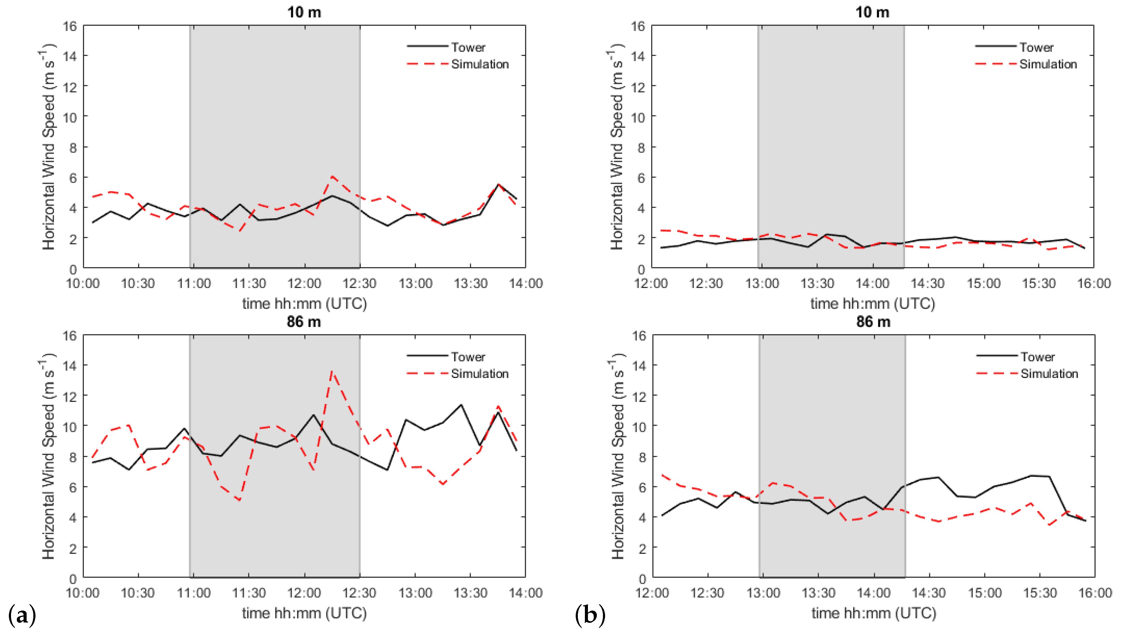
The simulation results are compared with measurements from cup anemometers and wind vanes installed on the mast. Time series of the 10-min averaged horizontal velocity and wind direction are shown in Figure 3 and Figure 4, respectively. The left panel of the following figures shows the results for the first day (21 September 2018), while the right one shows results for the second day (22 September 2018). The approximate times of the flights are indicated with a grey box in these figures for reference. On 21 September, the wind speed measurements ranged from 7 $\mathrm{m}{\mathrm{s}}^{-1}$ to 11 $\mathrm{m}{\mathrm{s}}^{-1}$ at 86 m a.g.l., while calmer wind conditions dominate the second day, with velocities between 4 $\mathrm{m}{\mathrm{s}}^{-1}$ and 7 $\mathrm{m}{\mathrm{s}}^{-1}$. The wind speed is in general well simulated, except for the upper level on the 21 September at 11:20 a.m. and 12:10 p.m. UTC and the first half an hour for the 22 September, where larger differences are observed. The simulated wind direction at upper levels is in accordance with the measured results. On 22 September, the wind direction near the ground shows high deviations. Indeed, values for wind direction at the EC-station show high variability even in the model, indicating a region of high turbulence and intermittent structures. The main flow is coming from west as shown by the relative constant value of 270$°$ at 86 m a.g.l., whereas, near the ground, the flow is more southerly orientated. This is clearly visible for the second day, with values reaching 200$°$ at 2:10 p.m. UTC.

It can be seen in Figure 3 and Figure 4 that, during the period of the flight campaign (marked with a grey box), the wind direction is remaining nearly constant between 240$°$ and 275$°$ for the first day and 265$°$ and 285$°$ for the second one. Only the wind speed shows a drop from 11 $\mathrm{m}{\mathrm{s}}^{-1}$ to 7 $\mathrm{m}{\mathrm{s}}^{-1}$ during the last 30 min for the first date. Except for the wind speed at 11:20 a.m. and 12:10 p.m. UTC on 21 September, the plots indicate a wind speed well simulated during the flight campaigns with values for mean absolute error at 100 m a.g.l. of 2.00 $\mathrm{m}{\mathrm{s}}^{-1}$ and 0.74 $\mathrm{m}{\mathrm{s}}^{-1}$ for the first and second day, respectively.

Turbulence is evaluated in terms of horizontal turbulence intensity (TI) given by the standard deviation of the horizontal wind speed normalized with the mean wind speed. Figure 5 compares the 10-min average simulated horizontal turbulence intensity against the measured data at 10 and 86 m a.g.l. The higher horizontal turbulence intensities are observed at the lower heights, i.e., at 10 m, with values above 40%. For 22 September, the TI values are even higher and can be explained by the definition of TI, which becomes large for small wind speeds. Several experimental [40,41] and numerical [42] studies have revealed that the maximum turbulent energy is produced in the upper half of the forest and carried into the region behind the forest [43,44]. For a westerly flow as in the present work, the 10 m sensor is located about 60 m downstream of the forested escarpment. This explains the high horizontal turbulence intensity values in comparison to the higher sensor at 86 m. The model simulates reasonably well the horizontal TI at the upper level and fails at catching the high values in the lower heights. The vegetative sink introduced by the canopy model [39] in the turbulence equations may be responsible and leads to an underestimate of the turbulent fluctuations. It should be reminded that TI is calculated with the data from a cup anemometer. As mentioned earlier, the sonic anemometers were not yet installed at that time. The influence of the vertical turbulence intensity is therefore not considered in this paper.

Figure 6 show 10-min averaged wind speed profiles at the tower position. The blue circles are data from the cup anemometers and the dashed lines the simulated wind speed. Error bars, corresponding to one standard deviation, are inserted for the anemometers’ measurements. Above 10 m, the standard deviations (error bars) are decreasing with height and reveal a greater variability at 45 m a.g.l. except for some specific times. The wind speed increases progressively with increasing height, with a visible wind speed reduction in the lower part of the profiles, i.e., at 10 m. On the first day, the wind speed at the lower cup anemometer is between 36 and 56% of the one at 100 m. The wind speed reduction is higher on the second day with ratio values ranging between 28 and 35%. Overall, the simulated and observed wind speed agree well in profile shape, except for some specific times.

4.2. Comparison with the UAS Measurements

The flight path consists of horizontal measurements legs made over and downstream of the escarpment, beginning at 20 m up to 200 m a.g.l. as shown in Figure 2. About 95 and 82 min were necessary to perform the complete flight path on 21 and 22 September 2018, respectively. Probes were placed in the CFD model at the leg positions and data are extracted for every simulation time step. For a direct comparison of the simulation results and the UAS measurements, the probes were selected in order to fit the flight time. The airborne wind measurements are then averaged over subsections of 20 m in length along each leg. Figure 7 illustrates the steepness of the terrain with a slope of around 20$°$. It also shows the position of the modelled forest in green and in blue the legs flown on both days. Except for the three upper altitudes, the patterns are almost similar between the two flight dates as shown in Figure 7a,b.

4.2.1. Wind Speed, Wind Direction and Inclination Angles

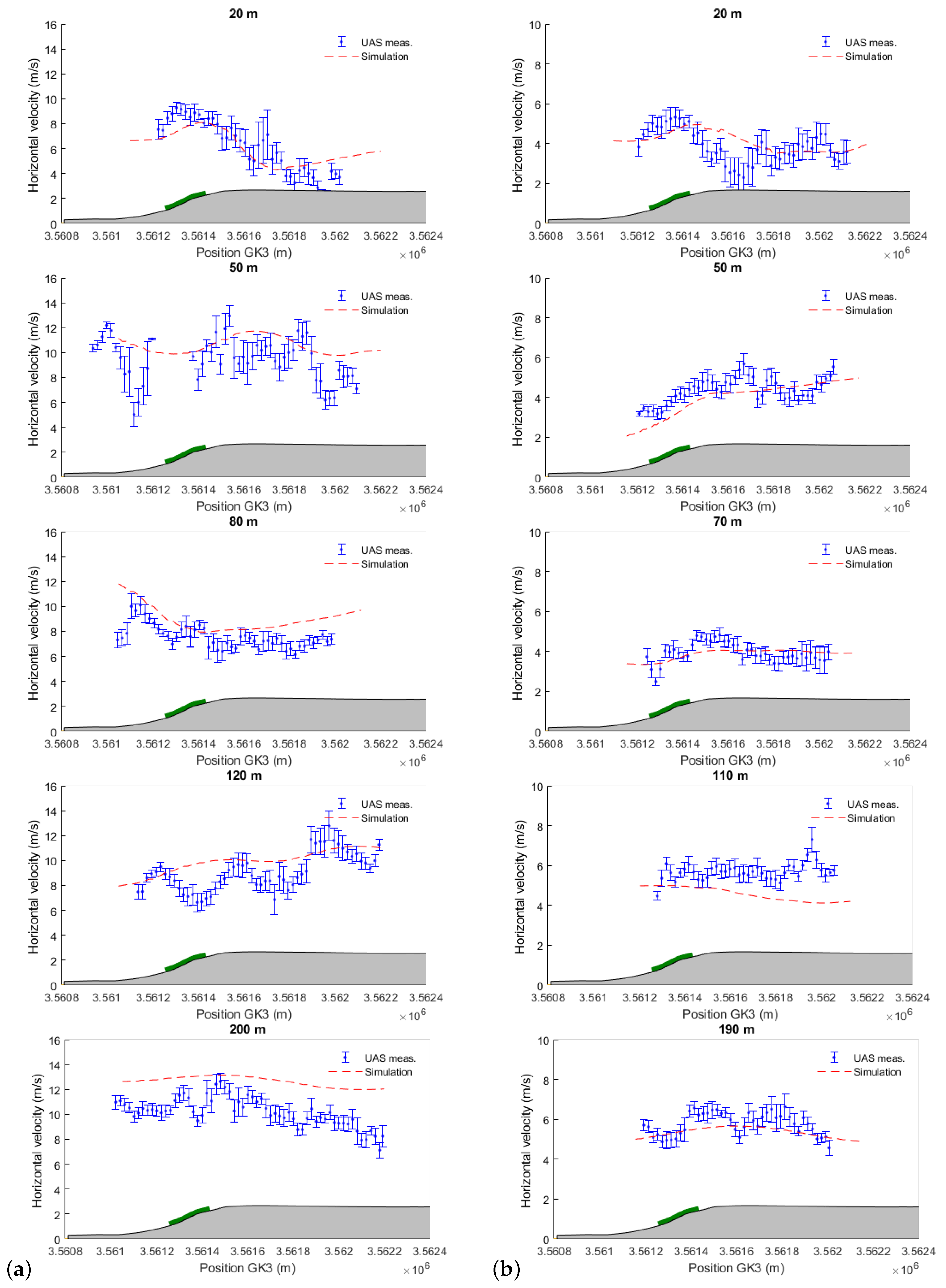
Figure 8 shows the horizontal wind speed at five different flight legs. For 21 September, levels at 20, 50, 80, 120 and 200 m a.g.l. were selected, while 20, 50, 70, 130 and 190 m a.g.l. were chosen for the second day. Error bars, corresponding to the standard deviation, are inserted for the UAS measurements. The standard deviations are binned over a window length of 20 m as well. The geometry of the ground and the position of the forested patch are added for better visualization. The scale for the velocity was deliberately changed for both days in order to give a better visualisation of the flow along the UAS paths. The measured velocities show a similar structure for both days: directly after the slope, the velocities are higher due to a local updraft generated by the orography. Behind the escarpment, at 20 m a.g.l., the velocity decreases rapidly to 3 $\mathrm{m}{\mathrm{s}}^{-1}$. Generally, the simulated wind speed matches the UAS measurements very well, with a slight overprediction at upper levels for the first day, as already observed in the time series in Figure 3.

Not only wind speed but also wind direction is a relevant parameter of wind power output. Several studies have shown that the occurrence of large directional change results in lower turbine performance [45,46]. The measured and simulated wind direction at the WINSENT test-site are presented in Figure 9. The profiles at higher altitudes are relatively flat, while the one at 20 m a.g.l. shows a sudden direction change right after the escarpment. For both days, the wind direction values are increasing with decreasing height, corresponding to a backing wind. For 21 September, the wind rotates up to 50$°$ between 20 and 200 m. However, it should not be forgotten that the flying time between 20 and 200 m are different: the measurements for the level at 20 m a.g.l. were performed at around 11:09 a.m. UTC and those at 200 m a.g.l. at around 12:26 p.m. UTC. The wind direction observed at the tower during the flight (grey box in Figure 4a) was about 260$°$ at the beginning and decreased to 230$°$ during the last 30 min. For the second day, the wind direction at the tower always keeps constant (around 270$°$ in Figure 4b) during the flight campaign. A backing wind with values reaching 20$°$ between 20 and 50 m is, however, visible in Figure 9b. The model performs well at upper levels, except for the first day where the backing is weaker.

Inclination angles are important for each turbine site: wind turbines have to be certified by the standards such as IEC 61400-1, where inflow angles are usually required to be within ±8$°$ [47]. The future turbine locations should comply with this requirement to ensure that the turbines will withstand the wear and tear during their expected lifetime. The modelled and measured inflow angles compared to each other are presented in Figure 10. Sudden changes in the inclination angle are numerically and experimentally noticed over the escarpment and are due to a local phenomenon induced by local features of the terrain. Positive flow angles of up to 15$°$, numerically, and 20$°$, experimentally, are reached. The position of this maximum reveals a flow dominated by upward movements and is located over or straight after the escarpment. It is noticeable that, for the second day, a negative angle can experimentally and numerically be seen in the last thirds of the flight path, indicating a flow not yet recovered. The flow remains disrupted even at upper levels (190 and 200 m a.g.l.), where inclination angle becomes smaller but still differs from zero. This reveals that the region of influence from the vegetated escarpment is not limited to low levels but extends to a region higher than the height of the escarpment itself. Previous wind tunnel experiments of escarpments with varying slope angles showed that the region of influence from an escarpment can go up to a height of 2 times the escarpment height [48,49].

As a surprise, the inclination angle is negative (i.e., a vertical wind component from above) at the beginning of the escarpment, even in the model, revealing an incoming flow that is already disturbed. For a westerly wind, the air passes over a small hill, located around 1.5 km west to the test-site (Figure 1a) and a recirculation can be expected in the valley, leading to negative inclination angles at the end of the valley and still at the beginning of the escarpment. The inclination angles then return to positive values at the upper edge of the escarpment as could be expected by an orographically influenced flow that follows the terrain. To check this hypothesis, the simulated vertical wind speeds in a cross-section along the legs for both days are shown in Figure 11. The simulated values are averaged over the complete flight campaign, i.e., 95 and 82 minutes. On 21 September, a large recirculation zone enclosed between the hill and the escarpment can be seen and corroborates our hypothesis.

The variability of the horizontal wind speed and inclination angle, indicated by the standard deviations, represent a measure of the turbulence intensity. Their values are larger at low altitudes in comparison to higher levels due to increased turbulence near the ground. Looking at the two lowest levels, it is even noticeable that the variability is greater right after the escarpment. This is in accordance with the observation from the meteorological tower in Figure 5. Despite the large differences in the wind condition (high and low wind speeds) for both days, the flow structure seems to be quite similar.

4.2.2. Stability Considerations

The stability can be characterized, e.g., using the potential temperature or the Richardson number. The assessment of atmospheric stability using ground stations and towers is difficult in complex terrain as the flow can be characterized by phenomena such as updraft, downdraft, or canopy flow. A UAS has the ability to sample the atmosphere at higher altitudes in comparison to ground-based instrumentation, and can be a tool for atmospheric stability measurement. In our study, the potential temperature and the bulk Richardson number are used to assess the stability behaviour at the test-site. The bulk Richardson number ${\mathrm{Ri}}_B$ [50], which can be computed from the wind and temperature measurement at two heights, is defined as:

$${\mathrm{Ri}}_B=\frac{g}{T_a}\frac{({\theta }_u-{\theta }_l)(z_u-z_l)}{{(U_u-U_l)}^2}$$

(7)

where $T_a$ is the average air temperature of the layer, ${\theta }_u$ and ${\theta }_l$ are the potential temperature at the upper $z_u$ and lower level $z_l$, respectively. U is the horizontal wind speed and g = 9.81 $\mathrm{m}{\mathrm{s}}^{-2}$ is the gravitational acceleration. There is still debate about the critical Richardson ${\mathrm{Ri}}_c$ values, but typically ${\mathrm{Ri}}_c=0.25$ for small $\Delta z$. For ${\mathrm{Ri}}_B<0.25$, the flow is probably unstable and turbulence is likely to occur.

The diurnal pattern of potential temperature over the entire two days by the tower is presented in Figure 12. For 21 September, the tower recorded very small vertical potential temperature gradients (also known as potential temperature lapse rate $\Delta \theta$/$\Delta z$) during the flight campaign, corresponding to near-neutral atmospheric conditions. During the flight campaign on 22 September, a negative lapse rate (calculated from 2 and 96 m) of −1.8 K/100 m is measured and indicates the occurrence of an unstable atmosphere. The sudden drop in the temperature at 4:00 p.m. UTC on 21 September due to a cold front has led to lower temperatures (around 10 K lower) on 22 September. In Figure 13, the bulk Richardson number at the mast is calculated using the mean wind speed and temperature data (10-min means), between 45 and 100 m a.g.l. During the periods of interest (grey box), the near neutral state on 21 September (${\mathrm{Ri}}_B\approx$ 0) and the unstable state on 22 September (${\mathrm{Ri}}_B\approx$−0.8) is clearly visible.

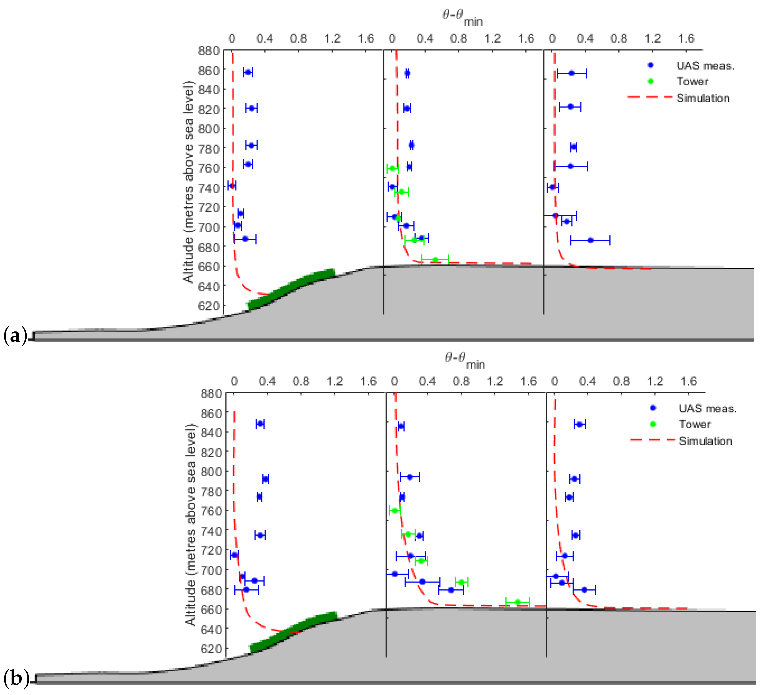
The potential temperature profiles from the tower, the MASC and the simulation are compared in Figure 14. Since potential temperature values are different for both days, the differences, that is, the potential temperature minus its minimum value ($\theta -{\theta }_{\min }$) are shown. The MASC measurements are separated in three regions: one over the escarpment, the second part is centred around the tower and the last region is further downstream. The simulation results are averaged over the whole flight duration. The potential temperature at all positions decreases with height. For the first day (Figure 14a), the region of decreasing temperature is visible in the lower 50 m, while, on the second day (Figure 14b), the layer up to 100 m is concerned. Above the escarpment, the simulation shows a potential temperature approaching neutral stratification at heights above 40 m a.g.l. The flight pattern is not following the terrain and therefore the lowest available measurement at this position is at 50 m a.g.l. In the middle region, the tower values (green dots) show a superadiabatic layer next to the ground, with a stronger temperature decrease with altitude on the second day. On that day, the potential temperature decreases by 1.5 K at the lowest 100 m. The MASC exhibits a decrease of 0.5 K between 20 and 50 m a.g.l. The agreement between the different systems (MASC and tower) is satisfactory, given the systematic differences in the measurement techniques, as well as in the vertical and temporal resolutions. The simulation shows a strong potential temperature decrease at the ground corresponding to the position of the first computational cell adjacent to the wall. Above the first cell, the decrease is slower and underestimated compared to measured data from the tower and MASC. This may be the result of a low vertical resolution near the ground but also the surface heat fluxes from the mesoscale model, which are underestimated around mid-day, i.e., during the measurement campaigns.

The bulk Richardson number based on a 20 m averaging windows is computed over the flight legs to assess the impact of the escarpment, with its forest, in enhancing critical conditions for shear instability. For the computations, three levels were chosen: a low level near the ground, a medium one and the highest flown altitudes. Figure 15 shows the distribution of the bulk Richardson’s number over the test-site. The drop in the bulk Richardson numbers right after the escarpment next to the ground (see ${\mathrm{Ri}}_B$ values between 20 and 120 m and between 20 and 110 m) for both days provide evidence for the criticality of the flow to shear instability and thus the generation of the turbulence. Thermodynamic instability near the ground associated with a turbulent wind flow leads to negative ${\mathrm{Ri}}_B$ values for both days. The bulk Richardson values are then stabilizing around 300 m behind the escarpment. On 21 September, it can be noticed that the bulk Richardson values computed at the upper levels (between 120 and 200 m) are around zero. This is explained by an increasing mechanical turbulence generated by large vertical wind shear. The mechanical shear at higher levels is not so strong on the second day, resulting in ${\mathrm{Ri}}_B$ values remaining negative and thus a layer always in an unstable state. The computed bulk Richardson values from the MASC are in accordance with the simulated values only for the first day. The stratification on the second day is numerically underestimated with a layer almost becoming dynamically stable ${\mathrm{Ri}}_B\ge$ 0.25) where it is, in fact, still unstable.

To summarize the results, it was found:

• Both days have a similar flow structure with a wind direction almost perpendicular to the escarpment. The main differences are the wind speed levels: strong and calm wind condition for the first and second day, respectively. The simulated wind speed and wind direction are in accordance with the tower measurements, except for some specific times. During the flight campaigns, values for mean absolute error of 2.00 $\mathrm{m}{\mathrm{s}}^{-1}$ and 0.74 $\mathrm{m}{\mathrm{s}}^{-1}$ are found for the first and second day, respectively. The tower, positioned 60 m behind the forest, clearly shows the impact of the forest with a wind speed in the lower levels (10 m a.g.l.) strongly reduced. The reduction is higher for 22 September, where the wind speed values at the lower cup are about one third of the one at 100 m, on average.
• The turbulence is evaluated in terms of horizontal turbulence intensity. The model simulates reasonably well at the upper levels but large discrepancies are observed in lower altitudes compared to the tower measurements. This may be directly linked to the canopy model. Possible future improvements require a deeper investigation on the plant canopy and the turbulence model. The influence of the vertical turbulence intensity is not considered in this paper, as no sonic anemometers were available at that time. Further work with the newly installed sonics is required to provide an accurate representation of the turbulence, including the vertical turbulence intensity.
• The UAS measurements are used for the model validation. In order to avoid any temporal averaging, a real-time strategy is applied, where the model follows spatially and temporally the aircraft. An accelerated flow is numerically and experimentally found over the escarpment. The model slightly over-predicts the wind speeds at higher levels for the first day but still matches very well the UAS measurements. The flow structure remains the same, despite a range of different velocities.
• Changes in wind direction at turbine heights can be easily measured by the MASC. At the WINSENT test-site, the wind turned counter-clockwise with height for both days, corresponding to a backing wind.
• Sonic anemometers mounted on a tower can provide the inclination angles. However these measurements are limited to the tower locations, and there can be significant discrepancies between the inclination angle at the tower location and the one at the turbine location. The MASC can overcome this problem and be used to probe the horizontal extent of an area with negative vertical wind, for example. Upward movements over and straight after the escarpment are observed. The inclination angles at an altitude of about 200 m are smaller but still not equal to 0$°$, indicating a flow still influenced by the orography and topography. Inclination angles of 5$°$ and 2$°$, at the future turbine location, are found for the first and second day, respectively. The test-site has been intentionally placed at a location that offers high inclination angles.
• The stability of the atmosphere can be described based on tower measurements, but the UAS offers the opportunity to sample at higher elevations. The calculated and simulated potential temperature profiles are in accordance with a near neutral ABL on the first day. The second day, dominated by a more convective surface layer, at the test-site is not well simulated. Indeed, the superadiabatic layer next to the ground is numerically underestimated. The temperature values at the ground in the OpenFOAM model are obtained by reading the surface heat fluxes from the WRF model and the low resolution (150 m) may be the reason of this underestimation. In future works, it will be interesting to nudge the CFD model with the EC measurements for the ground temperatures. The bulk Richardson values show a systematic drop behind the escarpment for layers near the ground and reveals thermodynamic instabilities.

5. Conclusions

In the present study, the flow over the WINSENT test-site was numerically and experimentally investigated for two days. Standard measuring systems such as a meteorological tower or an EC station, but also an unmanned aircraft system are used for the numerical validation. The CFD model, driven by the WRF data, relies on an unsteady RANS model with a canopy model for the forested areas. A simple one-way coupling approach shows good agreement with tower and EC measurements for the wind speed and wind direction. However, no acceptable accuracy for the turbulent intensity could be reached at the lower levels, where high wind shears are occurring, and, therefore, need to be more investigated.

The dataset provided by the airborne measurements demonstrates how an UAS system can be helpful for the ABL investigation by providing a high spatial resolution of the airflow near the escarpment. Numerical validation is performed by following the position of the MASC during the flight campaign, which takes more than an hour. In this way, the variation of the flow is caught and no time averaging is needed. A comparison of the horizontal wind speed, wind direction and inclination angle was able to determine the accuracy of our method. Generally, the simulated wind speed, direction and inclination angle match well with the MASC measurements. The stability characterization shows that the model is predicting well for the first day but need improvement for the second day, dominated by more unstable conditions. In the future, a flight strategy following the terrain should be implemented in order to get more information above the escarpment at lower altitudes. The UAS is still an exotic tool for wind resource assessment. This study provides confidence in using UAS as a tool for meteorological diagnostics or for data assimilation in models. A recently published study shows preliminary results from a WRF model, using assimilation of UAS data collected during the LAPSE-RATE Experiment [51]. The applied method shows improved prediction of wind speed and direction and is encouraging for future UAS data assimilation research.

A good level of accuracy is achievable by considering a CFD model, driven by a WRF model, at relatively low computational costs compared to large eddy simulations (LES) or detached eddy simulations (DES). The method presented in this paper will be extended by coupling the OpenFOAM model to a Delayed Detached Eddy Simulations (DDES) solver [33], where the future wind turbines will explicitly be included. In future, intensive observation periods with additional equipment, such as Lidars, and under stronger thermal stratifications will be performed.

References

1. Council of the European Union. Proposal for a Regulation of the European Parliament and of the Council Establishing the Framework for Achieving Climate Neutrality and Amending Regulation (EU) 2018/1999 (European Climate Law); Council of the European Union: Brussels, Belgium, 2020.
2. Fraile, D.; Komusanay, I. Wind Energy in Europe: Outlook to 2023; Technical Report; WIND Europe: Brussels, Belgium, 2019. [Google Scholar]
3. Jackson, P.S.; Hunt, J.C.R. Turbulent wind flow over a low hill. Q. J. R. Meteorol. Soc. 1975, 101, 929–955. [Google Scholar] [CrossRef]
4. Foken, T. 50 Years of the Monin–Obukhov Similarity Theory. Bound. Layer Meteorol. 2006, 119, 431–447. [Google Scholar] [CrossRef]
5. Haupt, S.E.; Kosovic, B.; Shaw, W.; Berg, L.K.; Churchfield, M.; Cline, J.; Draxl, C.; Ennis, B.; Koo, E.; Kotamarthi, R.; et al. On Bridging A Modeling Scale Gap: Mesoscale to Microscale Coupling for Wind Energy. Bull. Am. Meteorol. Soc. 2019, 100, 2533–2550. [Google Scholar] [CrossRef]
6. Dudhia, J. A history of mesoscale model development. Asia-Pac. J. Atmos. Sci. 2014, 50, 121–131. [Google Scholar] [CrossRef]
7. Jiménez, P.A.; Dudhia, J. Improving the Representation of Resolved and Unresolved Topographic Effects on Surface Wind in the WRF Model. J. Appl. Meteorol. Climatol. 2011, 51, 300–316. [Google Scholar] [CrossRef] [Green Version]
8. Flores-Maradiaga, A.; Benoit, R.; Masson, C. Enhanced modelling of the stratified atmospheric boundary layer over steep terrain for wind resource assessment. J. Phys. Conf. Ser. 2019, 1222, 012005. [Google Scholar] [CrossRef]
9. Tewari, M.; Kusaka, H.; Chen, F.; Coirier, W.J.; Kim, S.; Wyszogrodzki, A.A.; Warner, T.T. Impact of coupling a microscale computational fluid dynamics model with a mesoscale model on urban scale contaminant transport and dispersion. Atmos. Res. 2010, 96, 656–664. [Google Scholar] [CrossRef]
10. Kwak, K.H.; Baik, J.J.; Ryu, Y.H.; Lee, S.H. Urban air quality simulation in a high-rise building area using a CFD model coupled with mesoscale meteorological and chemistry-transport models. Atmos. Environ. 2015, 100, 167–177. [Google Scholar] [CrossRef]
11. Duraisamy, V.J.; Dupont, E.; Carissimo, B. Downscaling wind energy resource from mesoscale to microscale model and data assimilating field measurements. J. Phys. Conf. Ser. 2014, 555, 012031. [Google Scholar] [CrossRef]
12. Klaas, T.; Pauscher, L.; Callies, D. LiDAR-mast deviations in complex terrain and their simulation using CFD. Meteorol. Z. 2015, 24, 591–603. [Google Scholar] [CrossRef]
13. Santos, P.; Mann, J.; Vasiljevic, N.; Courtney, M.; Sanz Rodrigo, J.; Cantero, E.; Borbón, F.; Martínez-Villagrasa, D.; Martí, B.; Cuxart, J. The Alaiz Experiment (ALEX17): Wind Field and Turbulent Fluxes in a Large-Scale and Complex Topography with Synoptic Forcing; Technical University of Denmark: Kongens Lyngby, Denmark, 2019. [Google Scholar] [CrossRef]
14. Fernando, H.J.S.; Mann, J.; Palma, J.M.L.M.; Lundquist, J.K.; Barthelmie, R.J.; Belo-Pereira, M.; Brown, W.O.J.; Chow, F.K.; Gerz, T.; Hocut, C.M.; et al. The Perdigão: Peering into Microscale Details of Mountain Winds. Bull. Am. Meteorol. Soc. 2019, 100, 799–819. [Google Scholar] [CrossRef]
15. Shaw, W.J.; Berg, L.K.; Cline, J.; Draxl, C.; Djalalova, I.; Grimit, E.P.; Lundquist, J.K.; Marquis, M.; McCaa, J.; Olson, J.B.; et al. The Second Wind Forecast Improvement Project (WFIP2): General Overview. Bull. Am. Meteorol. Soc. 2019, 100, 1687–1699. [Google Scholar] [CrossRef]
16. Clifton, A.; Clive, P.; Gottschall, J.; Schlipf, D.; Simley, E.; Simmons, L.; Stein, D.; Trabucchi, D.; Vasiljevic, N.; Würth, I. IEA Wind Task 32: Wind Lidar Identifying and Mitigating Barriers to the Adoption of Wind Lidar. Remote Sens. 2018, 10, 406. [Google Scholar] [CrossRef] [Green Version]
17. Pauscher, L.; Vasiljevic, N.; Callies, D.; Lea, G.; Mann, J.; Klaas, T.; Hieronimus, J.; Gottschall, J.; Schwesig, A.; Kühn, M.; et al. An Inter-Comparison Study of Multi- and DBS Lidar Measurements in Complex Terrain. Remote Sens. 2016, 8, 782. [Google Scholar] [CrossRef] [Green Version]
18. Altstädter, B.; Platis, A.; Wehner, B.; Scholtz, A.; Wildmann, N.; Hermann, M.; Käthner, R.; Baars, H.; Bange, J.; Lampert, A. ALADINA—An unmanned research aircraft for observing vertical and horizontal distributions of ultrafine particles within the atmospheric boundary layer. Atmos. Meas. Tech. 2015, 8, 1627–1639. [Google Scholar] [CrossRef] [Green Version]
19. Platis, A.; Altstädter, B.; Wehner, B.; Wildmann, N.; Lampert, A.; Hermann, M.; Birmili, W.; Bange, J. An Observational Case Study on the Influence of Atmospheric Boundary-Layer Dynamics on New Particle Formation. Bound. Layer Meteorol. 2016, 158, 67–92. [Google Scholar] [CrossRef]
20. Cione, J.J.; Kalina, E.A.; Uhlhorn, E.W.; Farber, A.M.; Damiano, B. Coyote unmanned aircraft system observations in Hurricane Edouard (2014). Earth Space Sci. 2016, 3, 370–380. [Google Scholar] [CrossRef] [Green Version]
21. Wildmann, N.; Rau, G.A.; Bange, J. Observations of the Early Morning Boundary-Layer Transition with Small Remotely-Piloted Aircraft. Bound. Layer Meteorol. 2015, 157. [Google Scholar] [CrossRef]
22. Balsley, B.B.; Lawrence, D.A.; Woodman, R.F.; Fritts, D.C. Fine-Scale Characteristics of Temperature, Wind, and Turbulence in the Lower Atmosphere (0–1300 m) Over the South Peruvian Coast. Bound. Layer Meteorol. 2013, 147, 165–178. [Google Scholar] [CrossRef] [Green Version]
23. Kral, S.T.; Reuder, J.; Vihma, T.; Suomi, I.; O’Connor, E.; Kouznetsov, R.; Wrenger, B.; Rautenberg, A.; Urbancic, G.; Jonassen, M.O.; et al. Innovative Strategies for Observations in the Arctic Atmospheric Boundary Layer (ISOBAR)—The Hailuoto 2017 Campaign. Atmosphere 2018, 9, 268. [Google Scholar] [CrossRef] [Green Version]
24. Wildmann, N.; Bernard, S.; Bange, J. Measuring the local wind field at an escarpment using small remotely-piloted aircraft. Renew. Energy 2017, 103, 613–619. [Google Scholar] [CrossRef]
25. Mauz, M.; Rautenberg, A.; Platis, A.; Cormier, M.; Bange, J. First, identification and quantification of detached-tip vortices behind a wind energy converter using fixed-wing unmanned aircraft system. Wind Energy Sci. 2019, 4, 451–463. [Google Scholar] [CrossRef] [Green Version]
26. WindForS. WINSENT: Developing a Wind Energy Test Facility in Complex Terrain. Available online: www.windfors.de (accessed on 7 September 2020).
27. Weihing, P.; Schulz, C.; Lutz, T.; Krämer, E. Comparison of the Actuator Line Model with Fully Resolved Simulations in Complex Environmental Conditions. J. Phys. Conf. Ser. 2017, 854, 012049. [Google Scholar] [CrossRef]
28. Letzgus, P.; Lutz, T.; Krämer, E. Detached Eddy Simulations of the local Atmospheric Flow Field within a Forested Wind Energy Test Site located in Complex Terrain. J. Phys. Conf. Ser. 2018, 1037, 072043. [Google Scholar] [CrossRef]
29. Rautenberg, A.; Schön, M.; zum Berge, K.; Mauz, M.; Manz, P.; Platis, A.; van Kesteren, B.; Suomi, I.; Kral, S.T.; Bange, J. The Multi-Purpose Airborne Sensor Carrier MASC-3 for Wind and Turbulence Measurements in the Atmospheric Boundary Layer. Sensors 2019, 19, 2292. [Google Scholar] [CrossRef] [PubMed] [Green Version]
30. Hofsäß, M.; Clifton, A.; Cheng, P.W. Reducing the Uncertainty of Lidar Measurements in Complex Terrain Using a Linear Model Approach. Remote Sens. 2018, 10, 1465. [Google Scholar] [CrossRef] [Green Version]
31. Skamarock, W.C.; Klemp, J.B.; Dudhia, J.; Gill, D.O.; Barker, D.M.; Duda, M.G.; Huang, X.Y.; Wang, W.; Powers, J.G. A Description of the Advanced Research WRF Version 3. Available online: https://opensky.ucar.edu/islandora/object/technotes:500 (accessed on 7 September 2020).
32. Weller, H.G.; Tabor, G.; Jasak, H.; Fureby, C. A tensorial approach to computational continuum mechanics using object-oriented techniques. Comput. Phys. 1998, 12, 620. [Google Scholar] [CrossRef]
33. Kroll, N.; Eisfeld, B.; Bleecke, H.M. FLOWer. In Notes on Numerical Fluid Mechanics; Vieweg: Braunschweig, Germany, 1999; Volume 71, pp. 58–68. [Google Scholar]
34. Knaus, H.; Rautenberg, A.; Bange, J. Model comparison of two different non-hydrostatic formulations for the Navier-Stokes equations simulating wind flow in complex terrain. J. Wind Eng. Ind. Aerodyn. 2017, 169, 290–307. [Google Scholar] [CrossRef]
35. El Bahlouli, A.; Rautenberg, A.; Schön, M.; zum Berge, K.; Bange, J.; Knaus, H. Comparison of CFD Simulation to UAS Measurements for Wind Flows in Complex Terrain: Application to the WINSENT Test Site. Energies 2019, 12, 1992. [Google Scholar] [CrossRef] [Green Version]
36. Doms, G.; Baldauf, M. A Description of the Nonhydrostatic Regional COSMO-Model. 2018. Available online: http://www.cosmo-model.org/content/model/documentation/core/cosmoDyncsNumcs.pdf (accessed on 7 September 2020).
37. Dudhia, J. A Nonhydrostatic Version of the Penn State–NCAR Mesoscale Model: Validation Tests and Simulation of an Atlantic Cyclone and Cold Front. Mon. Weather Rev. 1993, 121, 1493–1513. [Google Scholar] [CrossRef] [Green Version]
38. Sogachev, A.; Kelly, M.; Leclerc, M.Y. Consistent Two-Equation Closure Modelling for Atmospheric Research: Buoyancy and Vegetation Implementations. Bound. Layer Meteorol. 2012, 145, 307–327. [Google Scholar] [CrossRef]
39. Katul, G.G.; Mahrt, L.; Poggi, D.; Sanz, C. ONE- and TWO-Equation Models for Canopy Turbulence. Bound. Layer Meteorol. 2004, 113, 81–109. [Google Scholar] [CrossRef] [Green Version]
40. Cionco, R.M. Intensity of turbulence within canopies with simple and complex roughness elements. Bound. Layer Meteorol. 1972, 2, 453–465. [Google Scholar] [CrossRef]
41. Shaw, R.H.; Den Hartog, G.; Neumann, H.H. Influence of foliar density and thermal stability on profiles of Reynolds stress and turbulence intensity in a deciduous forest. Bound. Layer Meteorol. 1988, 45, 391–409. [Google Scholar] [CrossRef]
42. Shaw, R.H.; Schumann, U. Large-eddy simulation of turbulent flow above and within a forest. Bound. Layer Meteorol. 1992, 61, 47–64. [Google Scholar] [CrossRef] [Green Version]
43. Liu, J.; Chen, J.M.; Black, T.A.; Novak, M.D. Eϵ modelling of turbulent air flow downwind of a model forest edge. Bound. Layer Meteorol. 1996, 77, 21–44. [Google Scholar] [CrossRef]
44. Aubrun, S.; Leitl, B. Development of an improved physical modelling of a forest area in a wind tunnel. Atmos. Environ. 2004, 38, 2797–2801. [Google Scholar] [CrossRef]
45. Murphy, P.; Lundquist, J.K.; Fleming, P. How wind speed shear and directional veer affect the power production of a megawatt-scale operational wind turbine. Wind Energy Sci. Discuss. 2019, 1–46. [Google Scholar] [CrossRef]
46. Sanchez Gomez, M.; Lundquist, J.K. The Effects of Wind Veer During the Morning and Evening Transitions. J. Phys. Conf. Ser. 2020, 1452, 012075. [Google Scholar] [CrossRef] [Green Version]
47. VDE VERLAG GMBH. DIN EN IEC 61400-1 VDE 0127-1:2019-12; Standards-VDE; VDE VERLAG GMBH: Berlin, Germany, 2019. [Google Scholar]
48. Bowen, A.J.; Lindley, D. A wind-tunnel investigation of the wind speed and turbulence characteristics close to the ground over various escarpment shapes. Bound. Layer Meteorol. 1977, 12, 259–271. [Google Scholar] [CrossRef]
49. Tsai, B.J.; Shiau, B.S. Experimental study on the flow charachteristics for wind over a two-dimensional upwind slope escarpment. J. Mar. Sci. Technol. 2011, 19, 7. [Google Scholar]
50. Stull, R.B. An Introduction to Boundary Layer Meteorology; Springer: Dutch, The Netherlands, 1988; pp. 1–27. [Google Scholar] [CrossRef]
51. De Boer, G.; Diehl, C.; Jacob, J.; Houston, A.; Smith, S.W.; Chilson, P.; Schmale, D.G.; Intrieri, J.; Pinto, J.; Elston, J.; et al. Development of Community, Capabilities, and Understanding through Unmanned Aircraft-Based Atmospheric Research: The LAPSE-RATE Campaign. Bull. Am. Meteorol. Soc. 2020, 101, E684–E699. [Google Scholar] [CrossRef] [Green Version]
Figure 1. (a) Orography with the blue box marking the test-site (Gauß-Krüger coordinates); (b) the different land uses applied in the simulations: red for urban, grey for ground and green for forest; (c) wind rose from 86 m at the test-site tower for the period of mid 2018–2019.
Energies 13 04688 g001
Figure 2. (a) View of the tower taken from east-southeast. To the west the tower is a dense canopy. This picture shows that the lowest anemometer (10 m) and the EC-station are directly downslope of the forest; (b) the flight patterns performed over the two days in September 2018. The colors along the legs indicate the measured horizontal wind speed. The red triangle marks the position of the tower and the yellow one is the EC-station. The white triangles are the future locations of the wind turbines.
Energies 13 04688 g002
Figure 3. Time series of 10-min averages of horizontal wind speed at 10 m and 86 m on 21 (a) and 22 (b) September. The time series for the simulation (red) and the tower observations (black) are shown. The grey box marks the time flight period.
Energies 13 04688 g003
Figure 4. Time series of 10-min averages of wind direction at 2 m and 86 m a.g.l. on 21 (a) and 22 (b) September. See also Figure 3.
Energies 13 04688 g004
Figure 5. Time series of 10-min averages of horizontal turbulence intensity at 10 m and 86 m on 21 (a) and 22 (b) September. See also Figure 3.
Energies 13 04688 g005
Figure 6. 10-min horizontal wind speed profiles for each hour at the tower on 21 (a) and 22 (b) September. Cup anemometer data are indicated with the blue circles and the simulation with the blue dashed lines.
Energies 13 04688 g006
Figure 7. Visualisation of the modelled ground. The blue lines correspond to the legs performed by the MASC on 21 (a) and 22 (b) September. The green block represents the modelled forest.
Energies 13 04688 g007
Figure 8. Horizontal velocity on 21 (a) and 22 (b) September at different altitudes along the UAS’s flight path. The blue dots are the UAS measurements and the red dashed lines are the simulation results. Error bars, corresponding to one standard deviation, are inserted for the MASC measurements. The green block represents the modelled forest.
Energies 13 04688 g008
Figure 9. Wind direction on 21 (a) and 22 (b) September at different altitudes along the UAS’ flight path. See also Figure 8.
Energies 13 04688 g009
Figure 10. Inclination angles on 21 (a) and 22 (b) September at different altitudes along the UAS’ flight path. See also Figure 8.
Energies 13 04688 g010
Figure 11. Cross-section of simulated vertical wind speed averaged over the whole flight duration on 21 (a) and 22 (b) September. The blue lines correspond to the legs plotted in Figure 8 and Figure 10 performed by the MASC.
Energies 13 04688 g011
Figure 12. Time series of 10-min averages of potential temperature on 21 (a) and 22 (b) September. The grey box marks the time flight periods.
Energies 13 04688 g012
Figure 13. Time series of 10-min averages of the Richardson number on 21 (a) and 22 (b) September. See also Figure 12.
Energies 13 04688 g013
Figure 14. Vertical profiles of potential temperature differences (potential temperature minus its minimum value) from the MASC (blue dots), the tower (green dots) and the simulation (red lines) over, behind and further downstream the escarpment on 21 (a) and 22 (b) September.
Energies 13 04688 g014
Figure 15. Bulk Richardson number computed from the UAS measurements on 21 (a) and 22 (b) September at different altitudes along the UAS’s flight path using 20 m horizontal intervals. The green block represents the modelled forest.
Energies 13 04688 g015