New Clearing Model to Mitigate the Non-Convexity in European Day-ahead Electricity Market


Abstract
:1. Introduction
1.1. Non-Convexities in the European Day-Ahead Electricity Market Model
1.1.1. Conventional Non-Convexity Issues
1.1.2. National Uniform Price in Italy
1.1.3. Current Solution
1.2. Literature Review
1.3. Approach and Contributions
- defines market rules for the input data to overcome the drawback of the make-whole payment mechanism in Europe, e.g., the “truth-telling” and the welfare sub-optimality;
- keeps shadow prices of the pure market solution to avoid the missing money since MCP is variable in the “minimum uplift approach” payments.
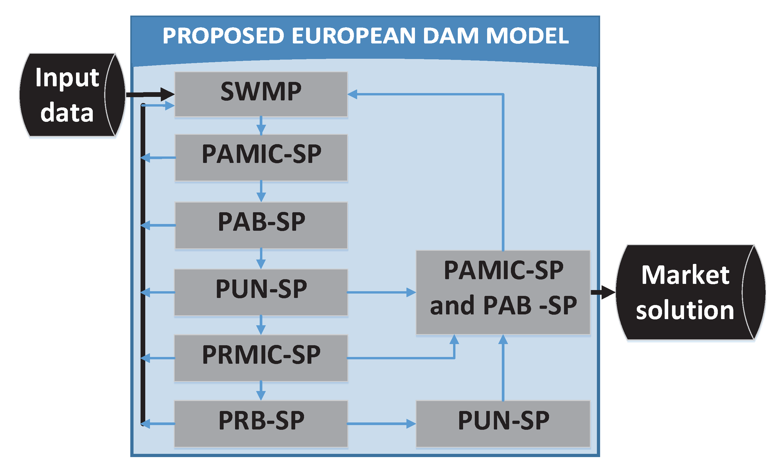
- The new European DAM model: the paper proposes an advanced model which contains all the market rules in Europe and provides the fair market solution in the minimum computation time;
- Improve the PUN-SP: because PUN is used for payment in for all PUN orders, it is impossible to introduce the “uplift” for each sub-order. Thus, the PUN-SP is improved by replacing the parametric optimization of the horizontal search with the cooperation between the “uplift” payments and final electricity prices to overcome the drawback of this optimization method that is the large computation time;
- Compute CR: provides a general formula to compute CR of interconnectors in Europe based on the dual variables of the network constraints where the losses of DC interconnectors and the meshed network are explicitly considered; and,
- Economic evaluation: the new payment scheme is carefully investigated and compared to the conventional payment method of [7] using the Western European case study, which is realistic case study in term of type and size of data. The analysis is performed considering various economic aspects to show that the proposal is acceptable at European level.
2. Mathematic Model
2.1. Verify Data
2.1.1. The Welfare Sub-Optimality
2.1.2. The Truth-Telling
2.2. Social Welfare Maximize Problem (SWMP)
2.2.1. Objective Function
2.2.2. Market Order Constraints
2.2.3. Power Balancing Equations
2.2.4. Network Constraints
2.3. PUN Search Sub-Problem (PUN-SP)
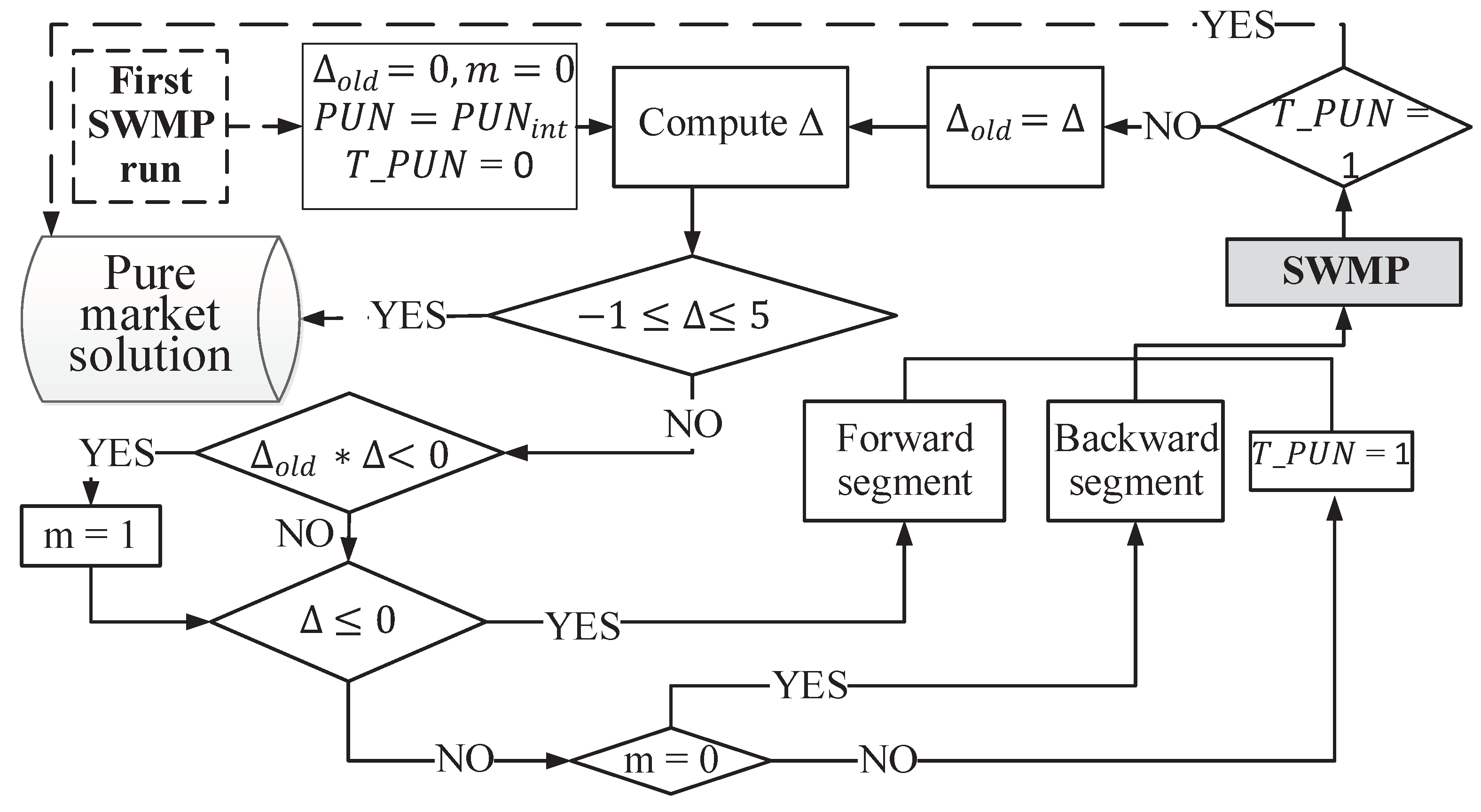
- Starting point: Initialization: is initialized as an empty set and the first run of SWMP is executed to obtain, among others, the accepted ratio and the zonal MCPs, i.e., ; following is initialize to (37) and is computed by (36). If is outside the tolerance ( [6]) initialize the Vertical search: (i) if is positive, select the backward vertical segment on the cumulated price-quantity curve of PUN orders with respect to the last accepted PUN order, while (ii) if is negative, select the forward segment on the cumulated price-quantity curve of PUN orders with respect to the last accepted PUN order and go to the Vertical search. If is inside the tolerance, exit PUN-SP.
- Vertical search: fix the demand in the PUN areas such that the bid price of accepted demand is higher or equal than , solve SWMP and compute using (36). (i) if the sign of is changed with respect to the previous iteration (from negative to positive side), the Horizontal search is executed and is set to 1 (14), else (ii) if is negative, select the forward segment, else select the backward segment; further, based on the selected vertical segment, update to a value within the selected vertical segment that minimizes ; finally, repeat Vertical search. If is inside the tolerance, PUN-SP stops.
- Horizontal search: fix to the bid price of the selected horizontal segment and define as the set of all demand segments for which . Subsequently, solve SWMP and stop PUN-SP (the dashed line in Figure 2).
2.4. Congestion Rent (CR)
2.5. Non-Uniform Price Problem (NUPP)
- although the non-convex bids are block and MIC orders, the model introduces “uplift” payment for all bids, i.e., for PUN orders and the CR of the TSO. The PUN orders need to be introduced as a insignificant variation of PUN can lead to very high variation in the total payment from PUN orders, bringing an important positive contribution to the payment scheme. Additionally, TSO can refuse an insignificant amount of congestion cost as an award for the new payment scheme;
- minimize the maximum “uplift” payment (), thus guarantying the consensus of all market players;
- an “uplift” payment can be a contribution or a subtraction: at the level of the market the net effect needs to be null so that the sum of all side-payments is equal to zero;
- the new payment must satisfy all the acceptance conditions; and,
- electricity price is a variable in this problem. Moreover, the relationship between the electricity prices of two areas needs to be preserved through the shadow price of the pure market solution.
2.5.1. Minimizing the Maximum Uplift Payment
2.5.2. Payment Balancing Equation
2.5.3. The Shadow Price and the Contribution of TSO
2.5.4. Constraints on the Payment
3. Results
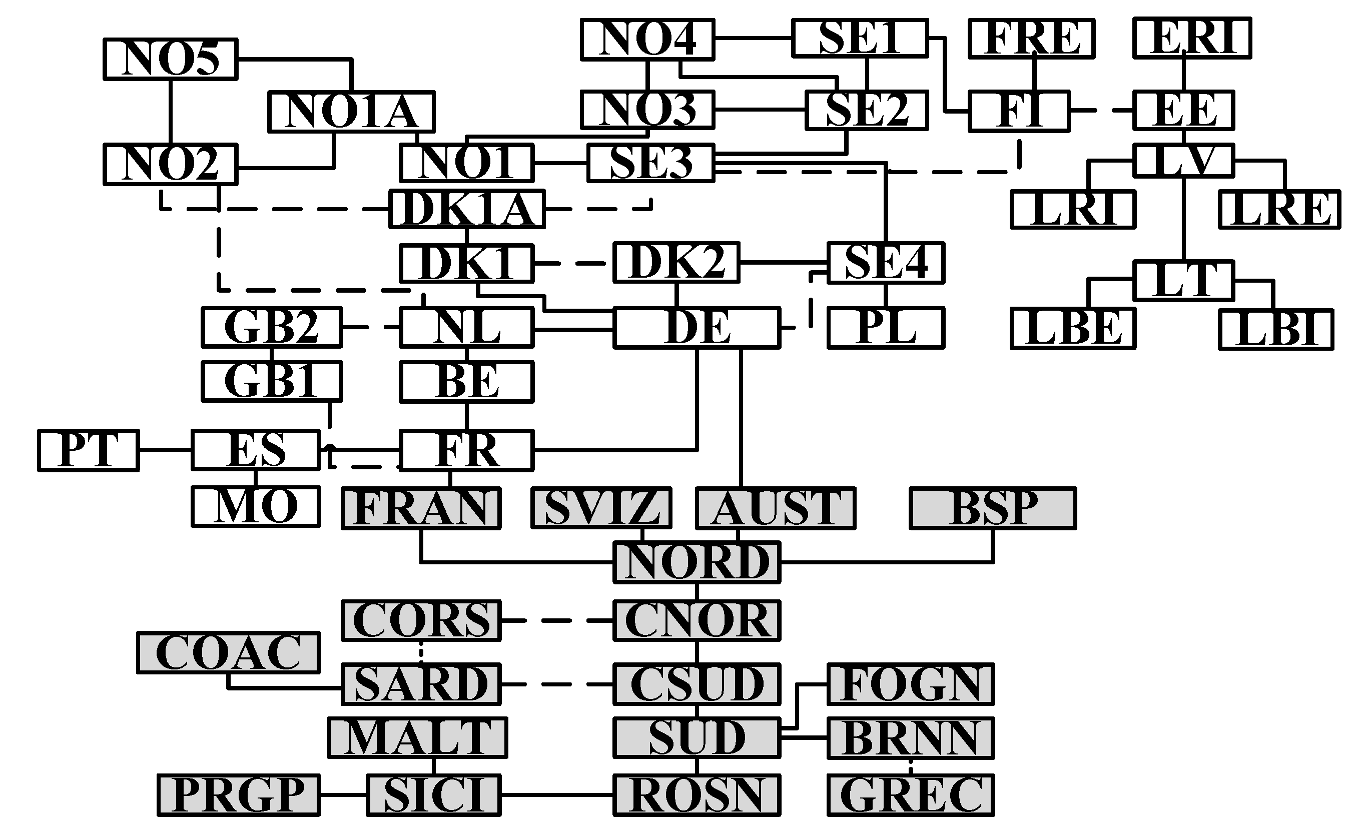
3.1. Case Studies Description
3.2. Artificial Case
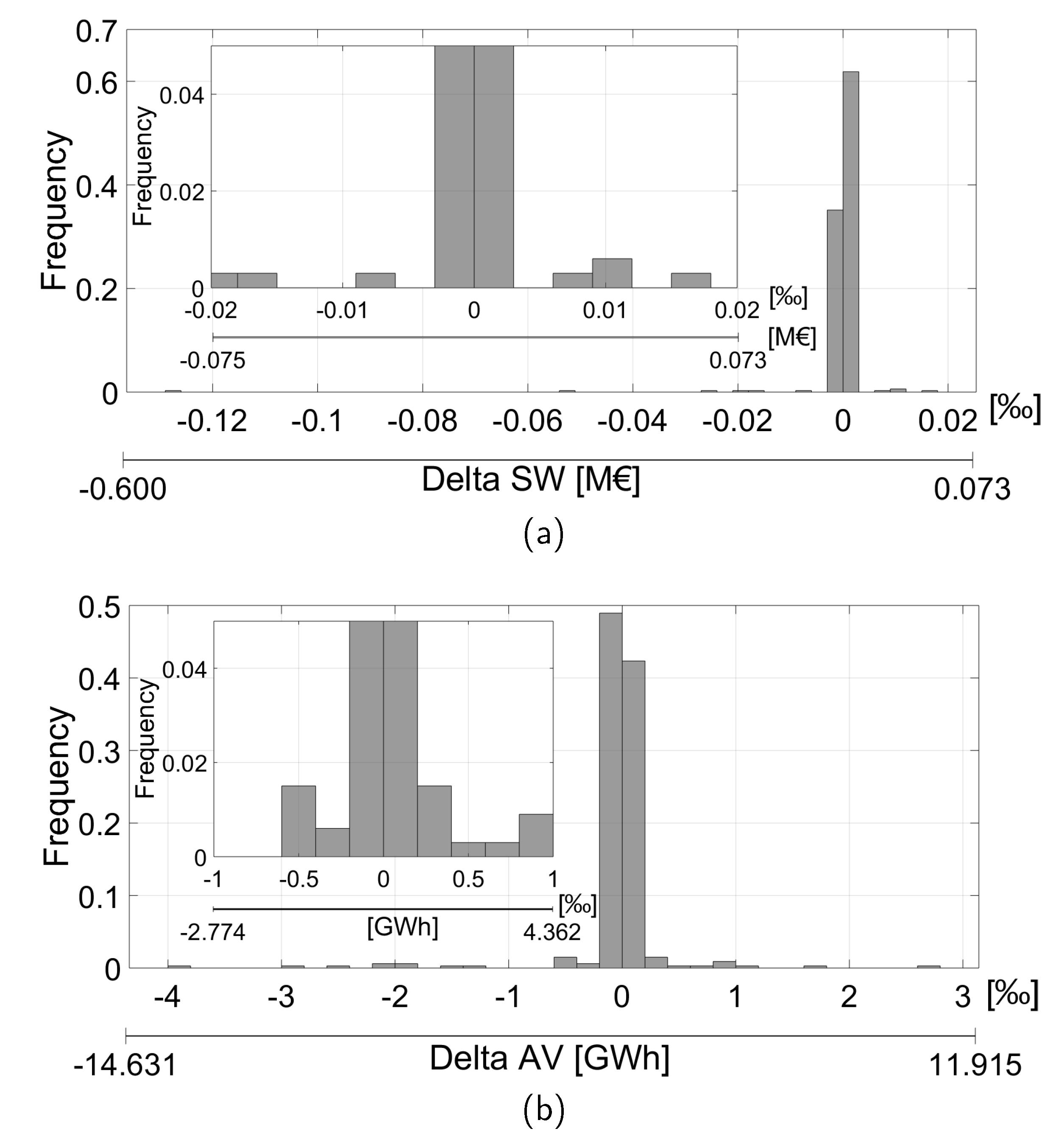
3.2.1. Global Criteria
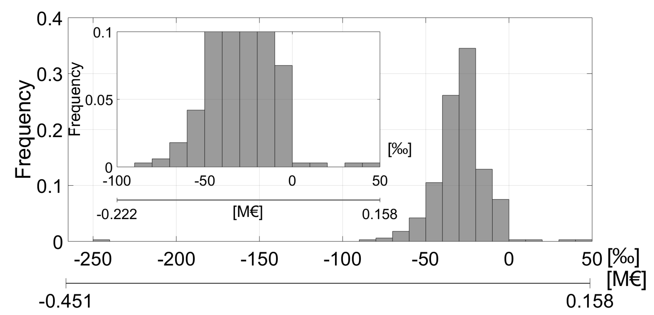
3.2.2. Economic Aspects
3.2.3. Impact on Orders
Block orders
Complex orders
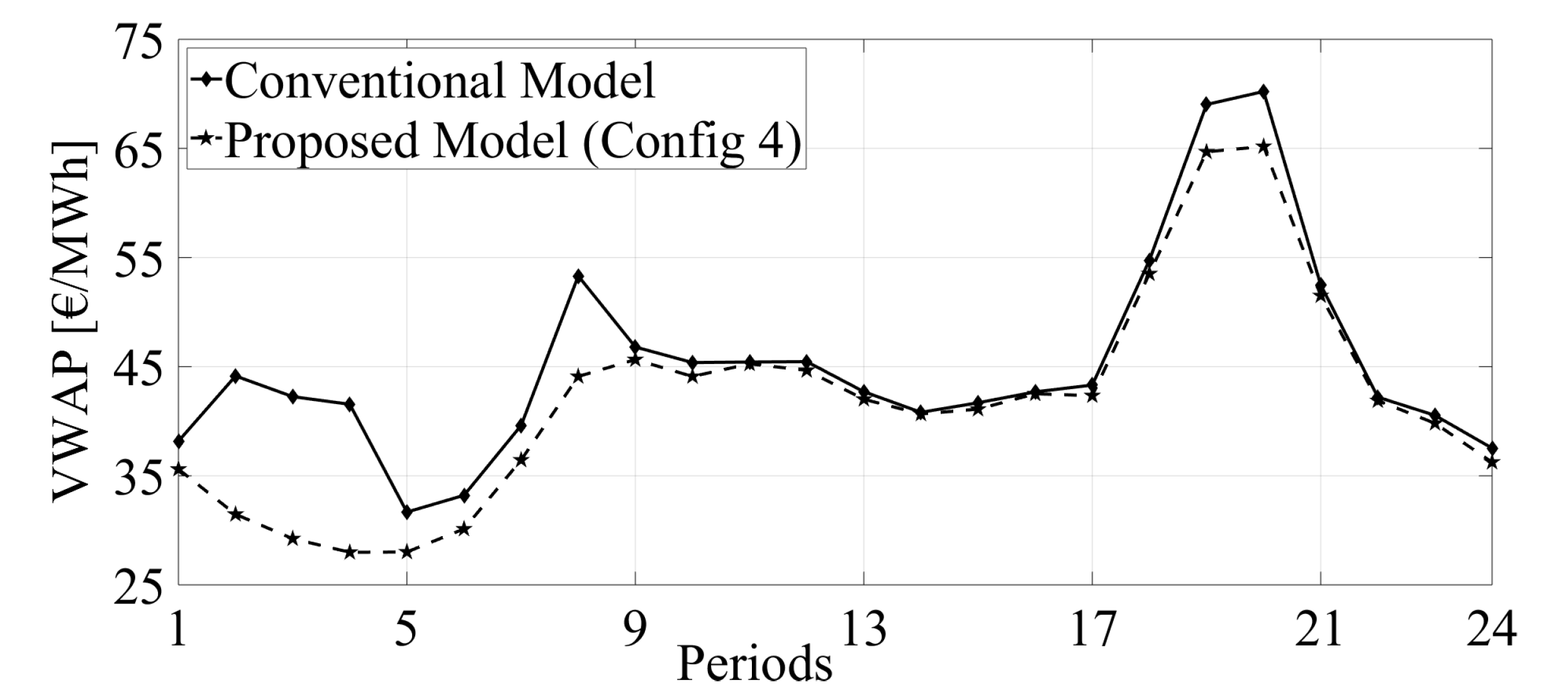
PUN orders
3.3. Real Data Case Study
4. Discussion
Author Contributions
Funding
Conflicts of Interest
Abbreviations
| Acronym | |
| DAM | Day-Ahead Market |
| PX | Power Exchange |
| EUPHEMIA | Pan-European Hybrid Electricity Market Integration Algorithm |
| MCP | Market Clearing Price |
| VWAP | Volume Weighted Average Price |
| MIC | Minimum Income Condition |
| SW | Social Welfare |
| PAMIC | Paradoxically Accepted MIC order |
| PAB | Paradoxically Accepted Block order |
| PRMIC | Paradoxically Rejected MIC order |
| PRB | Paradoxically Rejected Block order |
| SWMP | Social Welfare Maximize Problem |
| MIQP | Mixed-Integer Quadratic Program |
| SP | Sub-Problem |
| PAMIC-SP | Paradoxically Accepted Minimum Income Condition Sub-Problem |
| PAB-SP | Paradoxically Accepted Block Sub-Problem |
| PRMIC-SP | Paradoxically Rejected Minimum Income Condition Sub-Problem |
| PRB-SP | Paradoxically Rejected Block Sub-Problem |
| PUN | Prezzo Unico Nazionale (National Uniform Price) |
| PUN-SP | PUN search Sub-Problem |
| LGC | Load Gradient Condition |
| SSC | Schedule Stop Condition |
| NUPP | Non-Uniform Price Problem |
| ATC | Available Transfer Capacity |
| FB | Flow Based |
| CR | Congestion Rent |
| TSO | Transmission System Operator |
| NNS | Non-Negative Surplus |
| AV | Accepted Volume |
| Nomenclature | |
| Sets | |
| Set of dispatch periods in one day. | |
| Set of bidding areas includes all areas in Flow Based region and Available Transfer Capacity region, where . | |
| Sets of interconnectors | |
| Set of all critical branches. | |
| Set of interconnectors. l is defined by two areas, ( and imply the direction of power flow on interconectors, positive value if it goes from to and negative value if it goes from to ), where . Here, is subset of interconnectors in FB region, while is not in FB, including interconnectors between ATC areas and FB areas. | |
| Subset of interconectors in the same line set, . | |
| Set of Line Sets. | |
| Subset of interconnectors subjects to the hourly ramping constraint, . | |
| Subset of interconnectors loaded in period t. | |
| Sets of orders | |
| Set of hourly step orders submitted at area a, including stepwise and piecewise hourly supply orders , where . | |
| Subset of PUN orders, . | |
| Set of block orders submitted at area a. | |
| Set of small block orders in one block order b. | |
| Set of link block orders submitted at area a. | |
| Set of flexible hourly orders submitted at area a. | |
| Set of exclusive group orders submitted at area a. | |
| Set of producers at area a. Here, one producer submits an aggeration of step orders , . | |
| Set of producers in area a subject to Load Gradient Condition, Minimum Income Condition and Schedule Stop Condition, respectively, where , , . | |
| Parameters | |
| The value of submitted volume is positive for demand side and negative for supply side. | |
| Submitted price and volume of hourly step-wise order in period t, in €/MWh and MWh, respectively. | |
| Submitted price and volume of piecewise hourly order in period t, in €/MWh and MWh, respectively. | |
| Submitted price and volume of small block order in block order b in period t, in €/ MWh and MWh, respectively. | |
| Submitted price and volume of flexible block order in period t, in €/MWh and MWh, respectively. | |
| Starting (ending) unit steps of a small block order . Here, its value receives 1 if and receives 0 if , where shows the starting and ending time. | |
| Minimum acceptance ratio of block order b in p.u; where: for profile block order and for regular block order. | |
| Incidence matrix relating the link block order to its parent (when equal to 1), where . | |
| Incidence matrix relating the link block order to its family. Thus, the km-th element of is 1 if is the parent or child of , otherwise it is null. | |
| Fixed term (Variable term) of Minimum Income Condition of producer p in € (€/MWh), where . | |
| Binary parameter of sub-orders of producer subject to Schedule Stop Condition in period t, only it equals to 1 for the first sub-order in the first three periods. Limit capacity of interconnector l in period t in MWh, where . | |
| Initial total power of previous day of a in MWh. | |
| Hourly ramping up and down power limit of interconnector l, the line set , the area a in the period t in MWh/h and the daily ramping up and down of a in MW, respectively, where | |
| Power Transfer Distribution Factor (PTDF) of area a on critical branch in period t in p.u. | |
| Remain Available Margin (RAM) on critical branch in period t in MWh. | |
| The coefficient of interconnector l in €/MWh. | |
| Loss coefficient of interconnector l. | |
| Congestion rent of interconnector l in period t in €. | |
| Binary parameter relates to the positive and negative power flow in period t ( receives 1 for positive value and 0 for negative value; and vice versa with ). | |
| Continuous Variables | |
| The maximum of uplift payment in €/MWh. | |
| The accepted ratio of hourly step-wise , piece-wise , flexible order in period t. | |
| The uplift payment of hourly step-wise , piece-wise , small block , flexible order in period t in €/MWh. | |
| The accepted ratio of block order. | |
| National Uniform Price in period t. | |
| Net position of bidding area a in period t. | |
| Net position of bidding area a inside Flow Based region in period t. | |
| The uplift payment of congestion rent of interconnector l in period t in €/MWh. | |
| The uplift payment of PUN price in period t in €/MWh. | |
| Auxilary electricity price of area a in period t in €/MWh in the Non-Uniform Price Problem. | |
| Power flow and its positive and negative value on interconnector l in period t, where . | |
| Binary Variables | |
| Binary variable associated to block order b, and hourly flexible order in period t. | |
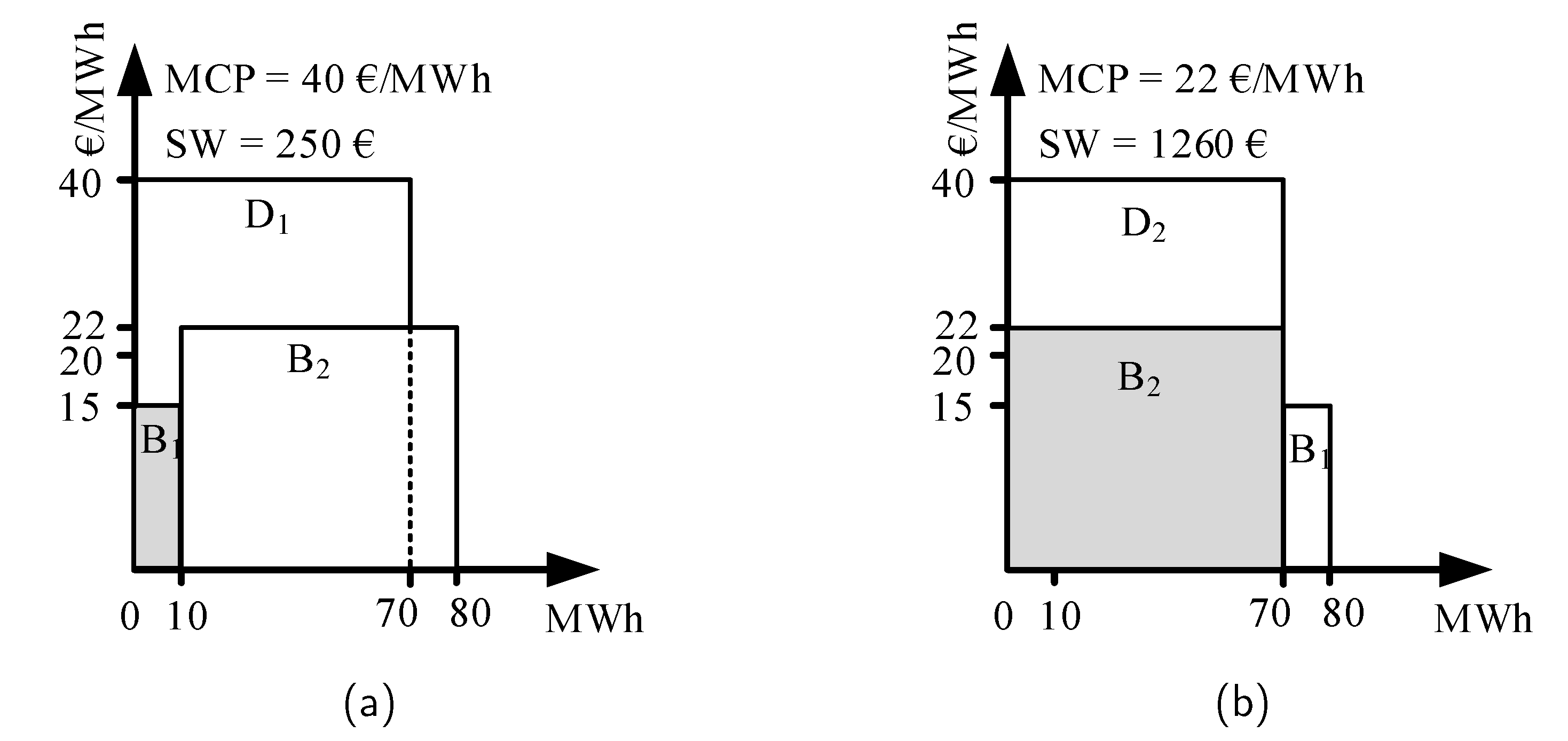
Appendix A. An Example of EUPHEMIA and New Market Solution
- Demand-D1 (Step): Q = 70 MWh and P = 40 €/MWh;
- Demand-D2 (Step): Q = 40 MWh and P = 20 €/MWh;
- Supply-B1 (Block - Fill-or-Kill): Q = −10 MWh and P = 15 €/MWh;
- Supply-B2 (Block - Fill-or-Kill): Q = −70 MWh and P = 22 €/MWh;
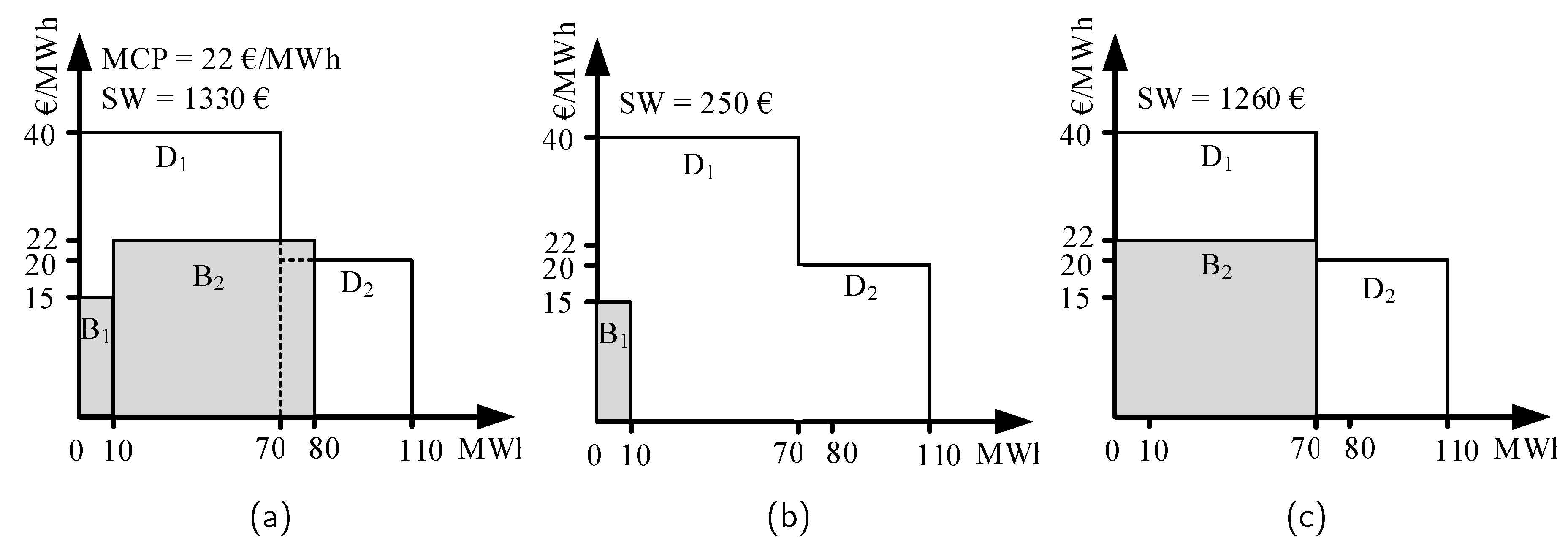
- D1 pays at 22.286 €/MWh;
- D2 pays at 20 €/MWh;
- B1 remunerates at 22 /MWh;
- B2 remunerates at 22 €/MWh.
Appendix B. The Functions of Orders
Appendix C. An Example of PRBs in the Proposed Model
References
- Le, H.L.; Ilea, V.; Bovo, C. Impact of the price coupling of regions project on the day-ahead electricity market in Italy. In Proceedings of the 2017 IEEE Manchester PowerTech, Manchester, UK, 18–22 June 2017; pp. 1–6. [Google Scholar] [CrossRef]
- Price Coupling of Regions. EUPHEMIA Public Description. 2016. Available online: https://www.bsp-southpool.com/files/documents/Zacasno/Euphemia%20Public%20Description%20version%20NEMO%20Committee.pdf (accessed on 15 July 2020).
- Le, H.L.; Ilea, V.; Bovo, C. Integrated European intra-day electricity market: Rules, modeling and analysis. Appl. Energy 2019, 238, 258–273. [Google Scholar] [CrossRef]
- ENTSO-E. Bidding Zone Configuration—Technical Report 2018. 2018. Available online: https://eepublicdownloads.blob.core.windows.net/public-cdn-container/clean-documents/events/2018/BZ_report/20181015_BZ_TR_FINAL.pdf (accessed on 22 April 2020).
- Bovo, C.; Ilea, V.; Carlini, E.; Caprabianca, M.; Quaglia, F.; Luzi, L.; Nuzzo, G. Review of the Mathematic Models to Calculate the Network Indicators to Define the Bidding Zones. In Proceedings of the 2019 54th International Universities Power Engineering Conference (UPEC), Bucharest, Romania, 3–6 September 2019; pp. 1–6. [Google Scholar]
- PCR Stakeholder. 2016. Available online: http://static.epexspot.com/document/34383/Euphemia%20Stakeholder%20Forum%20-%20presentation (accessed on 6 August 2020).
- Le, H.L.; Ilea, V.; Bovo, C. European day-ahead electricity market coupling: Discussion, modeling, and case study. Electr. Power Syst. Res. 2018, 155, 80–92. [Google Scholar] [CrossRef]
- GME. Appendix A: The Standard Hourly Auction Problem. 2002. Available online: https://www.mercatoelettrico.org/en/MenuBiblioteca/\Documenti/20041206UniformPurchase.pdf (accessed on 9 September 2020).
- Madani, M.; Vyve, M.V.; Marien, A.; Maenhoudt, M.; Luickx, P.; Tirez, A. Non-convexities in European day-ahead electricity markets: Belgium as a case study. In Proceedings of the 2016 13th International Conference on the European Energy Market (EEM), Porto, Portugal, 6–9 June 2016; pp. 1–5. [Google Scholar] [CrossRef]
- Vlachos, A.G.; Biskas, P.N. Adjustable Profile Blocks With Spatial Relations in the Day-Ahead Electricity Market. IEEE Trans. Power Syst. 2013, 28, 4578–4587. [Google Scholar] [CrossRef]
- Madani, M.; Vyve, M.V. Computationally efficient {MIP} formulation and algorithms for European day-ahead electricity market auctions. Eur. J. Oper. Res. 2015, 242, 580–593. [Google Scholar] [CrossRef]
- Chatzigiannis, D.I.; Dourbois, G.A.; Biskas, P.N.; Bakirtzis, A.G. European day-ahead electricity market clearing model. Electr. Power Syst. Res. 2016, 140, 225–239. [Google Scholar] [CrossRef]
- Sleisz, A.; Raisz, D. Complex supply orders with ramping limitations and shadow pricing on the all-European day-ahead electricity market. Int. J. Electr. Power Energy Syst. 2016, 83, 26–32. [Google Scholar] [CrossRef]
- Ruiz, C.; Conejo, A.J.; Gabriel, S.A. Pricing Non-Convexities in an Electricity Pool. IEEE Trans. Power Syst. 2012, 27, 1334–1342. [Google Scholar] [CrossRef]
- Hogan, W.W.; Ring, B.J. On Minimum-Uplift Pricing for Electricity Markets. Electricity Policy Group. 2003, pp. 1–30. Available online: https://scholar.harvard.edu/whogan/files/minuplift_031903.pdf (accessed on 9 September 2020).
- Savelli, I.; Giannitrapani, A.; Paoletti, S.; Vicino, A. An optimization model for the electricity market clearing problem with uniform purchase price and zonal selling prices. IEEE Trans. Power Syst. 2018, 33, 2864–2873. [Google Scholar]
- Savelli, I.; Cornélusse, B.; Giannitrapani, A.; Paoletti, S.; Vicino, A. A new approach to electricity market clearing with uniform purchase price and curtailable block orders. Appl. Energy 2018, 226, 618–630. [Google Scholar] [CrossRef] [Green Version]
- Le, H.L.; Ilea, V.; Bovo, C. A Thorough Comparison Among Various Mathematical Approaches to Compute PUN in Italy. In Proceedings of the 2018 15th International Conference on the European Energy Market (EEM), Lodz, Poland, 27–29 June 2018; pp. 1–5. [Google Scholar]
- Chatzigiannis, D.I.; Biskas, P.N.; Dourbois, G.A. European-type electricity market clearing model incorporating PUN orders. IEEE Trans. Power Syst. 2016, 32, 261–273. [Google Scholar]
- O’Neill, R.P.; Sotkiewicz, P.M.; Hobbs, B.F.; Rothkopf, M.H.; Stewart, W.R., Jr. Efficient market-clearing prices in markets with nonconvexities. Eur. J. Oper. Res. 2005, 164, 269–285. [Google Scholar] [CrossRef] [Green Version]
- Van Vyve, M. Linear Prices for Non-Convex Electricity Markets: Models and Algorithms; Technical Report; CORE: Leuven, Belgium, 2011. [Google Scholar]
- Zoltowska, I. Direct Minimum-Uplift Model for Pricing Pool-Based Auction With Network Constraints. IEEE Trans. Power Syst. 2016, 31, 2538–2545. [Google Scholar] [CrossRef]
- N_SIDE. Non-Uniform Pricing and Thermal Orders for the Day-Ahead Market. 2016. Available online: https://www.nordpoolgroup.com/globalassets/download-center/single-day-ahead-coupling/nonuniformpricingandthermalorders.pdf (accessed on 6 August 2020).
- EPEXSPOT. Blocks Parameters in ETS. 2016. Available online: https://www.epexspot.com/en/regulation (accessed on 9 September 2020).
- Gazette, S.O.S. Daily and Intraday Electricity Market Operating Rules. 2015. Available online: https://www.omie.es/sites/default/files/2019-12/20151223_reglas_mercado_ingles.pdf (accessed on 9 September 2020).
- Amprion, A.; Belpex, C.; Elia, E.; RTE, T.; Transnet, B. Documentation of the CWE FB MC Solution: As Basis for the Formal Approval-Request. Technical Report. 2014. Available online: https://www.acm.nl/sites/default/files/old_publication/bijlagen/13001_140530-cwe-fb-mc-formal-approval-request.pdf (accessed on 6 August 2020).
- Sleisz, A.; Raisz, D. Integrated mathematical model for uniform purchase prices on multi-zonal power exchanges. Electr. Power Syst. Res. 2017, 147, 10–21. [Google Scholar] [CrossRef]
- ENTSO-E ENTSO-E Transmission System Map. Available online: https://www.entsoe.eu/data/map/ (accessed on 9 September 2020).
- Pool, N. Trading Capacities. Available online: https://www.nordpoolgroup.com/Market-data1/#/nordic/table (accessed on 9 August 2020).
- Platform, E.T. Transmission. Available online: https://transparency.entsoe.eu/transmission-domain/r2/implicitAllocationsDayAhead/show (accessed on 9 September 2020).
- EPEX. Order Market Data. Available online: https://webshop.eex-group.com (accessed on 9 September 2020).
- OMIE. Market Results. Available online: https://www.omie.es/en/market-results/daily/daily-market/aggragate-suply-curves (accessed on 9 September 2020).
- GME, Downloads—Data—MGP Conventional Prices. Available online: http://www.mercatoelettrico.org/En/download/\DownloadDati.aspx?val=MGP_PrezziConvenzionali (accessed on 9 August 2020).
- GAMS, General Algebraic Modeling System. Available online: https://www.gams.com/ (accessed on 9 August 2020).


| Model | Welfare | Volume | Time | NNS [M€] | |
|---|---|---|---|---|---|
| [M€] | [GWh] | [min] | Supply | Demand | |
| Conventional | 6821.42 | 6935.97 | 90 | _ | _ |
| Proposed | 6822.36 | 6968.58 | 5 | 152.81 | 4070.02 |
| Config | TSO | PUN | Max_ | |||
|---|---|---|---|---|---|---|
| [‰] | [‰] | [%] | [€/MWh] | |||
| 1 | No | No | +0.194 | −0.0139 | 0.0 | 0.0224 |
| 2 | No | Yes | −0.337 | +0.0087 | 0.0 | 0.0198 |
| 3 | Yes | No | −0.330 | +0.0095 | 0.225 | 0.0223 |
| 4 | Yes | Yes | −0.324 | +0.0092 | 0.2 | 0.0197 |
| Average Value | Min Value [Month] | Max Value [Month] |
|---|---|---|
| 10.32% | 7.63% [August] | 13.66% [March] |
| Model | Average Value | Min Value [Day] | Max Value [Day] |
|---|---|---|---|
| [s] | [s] | [s] | |
| Conventional | 453 | 48 [26th of April] | 4532 [20th of July] |
| Proposed | 337 | 88 [31th of July] | 1448 [4th of November] |
| Average Value | Min Value | Max Value |
|---|---|---|
| 0.0036 | 1.5427 × 10⁻⁷ | 0.0888 |
© 2020 by the authors. Licensee MDPI, Basel, Switzerland. This article is an open access article distributed under the terms and conditions of the Creative Commons Attribution (CC BY) license (http://creativecommons.org/licenses/by/4.0/).
Share and Cite
Hong Lam, L.; Ilea, V.; Bovo, C. New Clearing Model to Mitigate the Non-Convexity in European Day-ahead Electricity Market. Energies 2020, 13, 4716. https://doi.org/10.3390/en13184716
Hong Lam L, Ilea V, Bovo C. New Clearing Model to Mitigate the Non-Convexity in European Day-ahead Electricity Market. Energies. 2020; 13(18):4716. https://doi.org/10.3390/en13184716
Chicago/Turabian StyleHong Lam, Le, Valentin Ilea, and Cristian Bovo. 2020. "New Clearing Model to Mitigate the Non-Convexity in European Day-ahead Electricity Market" Energies 13, no. 18: 4716. https://doi.org/10.3390/en13184716
APA StyleHong Lam, L., Ilea, V., & Bovo, C. (2020). New Clearing Model to Mitigate the Non-Convexity in European Day-ahead Electricity Market. Energies, 13(18), 4716. https://doi.org/10.3390/en13184716